• Aucun résultat trouvé

On the amount of regularization for super-resolution reconstruction

N/A
N/A
Protected

Academic year: 2021

Partager "On the amount of regularization for super-resolution reconstruction"

Copied!
12
0
0

Texte intégral

(1)

HAL Id: hal-00763984

https://hal.archives-ouvertes.fr/hal-00763984v2

Submitted on 24 Oct 2013

HAL is a multi-disciplinary open access

archive for the deposit and dissemination of

sci-entific research documents, whether they are

pub-lished or not. The documents may come from

teaching and research institutions in France or

abroad, or from public or private research centers.

L’archive ouverte pluridisciplinaire HAL, est

destinée au dépôt et à la diffusion de documents

scientifiques de niveau recherche, publiés ou non,

émanant des établissements d’enseignement et de

recherche français ou étrangers, des laboratoires

publics ou privés.

reconstruction

Yann Traonmilin, Saïd Ladjal, Andrés Almansa

To cite this version:

Yann Traonmilin, Saïd Ladjal, Andrés Almansa. On the amount of regularization for super-resolution

reconstruction. [Research Report] Telecom ParisTech. 2012. �hal-00763984v2�

(2)

On the amount of regularization for super-resolution

reconstruction

Yann Traonmilin*, Sa¨ıd Ladjal, Andr´es Almansa

Abstract—Modern digital cameras are quickly reaching the fundamental physical limit of their native resolution. Super-resolution (SR) aims at overcoming this limit. SR combines several images of the same scene into a high resolution image by using differences in sampling caused by camera motion. The main difficulty encountered when designing SR algorithms is the ill-posedness of the general SR problem. Assumptions on the regularity of the image are then needed to perform SR. Thanks to advances in regularization priors for natural images, producing visually plausible images becomes possible. However, regularization may cause a loss of details. Therefore, we argue that regularization should be avoided when possible, especially when the restored image is needed for further precise processing. This paper provides principles guiding the local choice of regularization parameters for SR. With this aim, we give an invertibility condition for affine SR interpolation. When this condition holds, we study the conditioning of the interpolation and affine motion estimation problems. We show that these problems are more likely to be well posed for a large number of images, leading to the possibility of a regularization-free super-resolution. When conditioning is bad, we propose a local total variation regularization for interpolation and show its application to multi-image demosaicking.

EDICS : TEC-ISR Interpolation, Super-Resolution and Mo-saicing: Interpolation and superresolution; Mosaicing, registra-tion and alignment; Multi-image fusion

I. INTRODUCTION

A. Problem statement and state of the art

Super-resolution aims at recovering a high resolution (HR) image from several low resolution (LR) images. In the most generic formulation of SR, we need to estimate camera blur, motion and the HR image simultaneously, which is an ill-posed problem. SR techniques have been reviewed several times in the literature [1], [2]. They mostly rely on a regularized minimization of a functional linking the acquired LR images and the unknown HR image. There is a wide choice of such functionals, including L2 norm with

Tychonov regularization [3], bilateral total variation (TV) regularization [4], [5], and L1 norm with TV regularization

[6], [7]. The choice of a regularizer is an implicit hypothesis (or a priori information) on the content of the image. For example, perfect reconstruction with TV regularization is not possible if the image contains too many textures [8], [9]. Even recent non-local regularization methods for single and multi-image super-resolution [10], [11] need images which

Y. Traonmilin, S. Ladjal and A. Almansa (email:

{yann.traonmilin,ladjal,andres.almansa}@telecom-paristech.fr) are with

Telecom ParisTech, CNRS LTCI, 46 rue Barrault, 75013 Paris, France. Tel: +33145817777

Work partially funded by FUI-9 CEDCA project.

exhibit rotational [12] or multiscale [13] self-similarities. When these hypotheses are not met, regularization fails to recover perfectly the high resolution image. Our aim is to recover as much of the HR image as possible. To achieve this, we will avoid or minimize assumptions made on the HR image, and consequently minimize the amount of regularization.

The relative motion between LR images is often restricted to translations and rotations. However, a small motion of the camera in the depth direction can cause a linear zoom between images. To describe this, we will consider affine motions of the LR sampling grids. Affine motions have been considered in [14]–[16] where conventional techniques for parameter estimation and regularized reconstruction are described. As we study the well-posedness of the SR problem, we will not invert camera blur as this part of the SR problem is generally ill-posed. With this configuration, super-resolution can be split in two processes: (i) interpolation (i.e. SR inversion with known motion parameters) and (ii) motion parameter estimation. In the interpolation case, super-resolution is an irregular to regular sampling interpolation problem which could be solved with general techniques [17]–[20]. With super-resolution sampling configurations, we can use the fact that each LR image is acquired on a regular grid to obtain dedicated results and methods. For example, the pure translational case can be viewed as a multichannel sampling problem. Thus, extending the result of Papoulis [21], Ahuja and Bose [22] showed that if we have a super-resolution factor M , only M2 LR images with pure translational

motions are needed to perfectly recover the HR image in a noiseless set-up. In this case, no assumption on the content of the HR image is needed (apart from the fact that it is band-limited). It naturally leads to the following question: in what conditions on the acquisition system can we perform super-resolution without hypotheses on the image?

The other side of the SR reconstruction problem is the registration of each LR image. It consists in estimating motion parameters between LR images (6 parameters for each affine motion). Some techniques for affine motion estimation between a pair of well-sampled images already exist [23]. However, in a non-trivial super-resolution set-up, LR images are assumed to be aliased, and these methods do not give estimates precise enough to perform a good reconstruction [24], [25]. If the interpolation problem is invertible, SR reconstruction can be viewed as a non-linear minimization problem with respect to motion parameters which is called variable projection [26]. [27] showed that using a regularized variable projection method for

(3)

super-resolution reconstruction gives stable results in practice. However, the necessity for a regularization term in the variable projection method is not questioned.

When the acquired data is contaminated by noise, having a good conditioning of the system is critical for the quality of the reconstructed image. The influence of the SR zoom has been studied in the case of interpolation in [28]. Experiments on the Cramer-Rao bound with respect to the number of images were shown by Robinson [25] and Champagnat [29], demonstrating that the reconstruction error of the pseudo-inverse decreases when the number of images grows.

B. Overview and Contributions

In this paper, we first describe (Section II) the theoretical context of super-resolution with affine motion, which requires special attention in terms of how hypotheses are formulated, and under which conditions the super-resolution, denoising and deconvolution problems can be decoupled from one another. Within this framework, we give in Section III a sufficient condition on the invertibility of SR interpolation. This extends the work of Ahuja [22] (which is restricted to translational motions) to the invertibility of affine motion SR interpolation. This result shows that the number of samples needed for affine SR with random motions is the same as the one for random sampling of trigonometric polynomials as shown by Bass & Gr¨ochenig [30]. In Section IV, the asymptotic behaviour of translational SR interpolation shown by Champagnat [29] is extended to affine motions. We show that it is in the interest of acquisition system designers to target the acquisition of a large number of LR images, as the SR reconstruction is likely to be well-posed in that setting. We also study the registration for large number of images by calculating the Hessian of the non-linear least squares motion parameter estimation problem. It allows for a better understanding of how variable projection behaves and shows that a regularization term (like in [27]) is not always necessary. We prove with real images taken with a hand-held camera that taking more images allows for the recovery of the true content of the image, without regularization. In Section V, we show that the conditioning is spatially varying. We calculate this conditioning for small motions and use it to predict how SR interpolation must be regularized. This prediction takes the form of a new local weighting scheme of the total variation regularizer. Finally, we apply it to multi-image demosaicking. We show that regularization and cross-channel dependencies used by even the most advanced demosaicking algorithms can be avoided if multiple images are available. In this case regularization assumptions are minimized by our procedure, and demosaicking artifacts are avoided.

II. THEORETICAL CONSIDERATIONS

A. Problem set-up

The purpose of the super-resolution problem is to invert a linear map A that produces N LR images from a single HR

image:

A : (CM L×ML) → (CL×L)N

u → (SQiu)i=1,N

(1) where N is the number of LR images, M is the super resolution factor, L × L is the size of a LR image, u is the HR image.S is the sub-sampling operator by a factor M and Qiare the affine deformation associated with each LR image.

We call qi the corresponding affine motion of the sampling

grid i.e.

(Qiu)(x) = u(qi(x)). (2)

We decompose qi in its linear and translational parts:

qix = lix+ ti. li are 2 × 2 matrices, ti are 2 dimensional

vectors. SR is the process of recoveringu from w = Au + n (n is acquisition noise). If the Qi are known, the inversion of

A is called the super-resolution interpolation. The recovery of bothu and Qi is called super-resolution reconstruction.

B. Hypotheses

We make assumptions on the problem to simplify the study: 1) u is band-limited

2) the first LR image is the reference image (Q1= Id)

3) affine maps on the coordinates (qi) are invertible

4) affine maps do not generate aliasing on the HR grid Condition 1) is always fulfilled because diffraction caused by the physical aperture of the camera act as a perfect low-pass filter. In practice, a maximum SR factor of 2 to 4 can be considered (see [31]). Condition 2) and 3) are always met when affine motion are not degenerate. Condition 4) deserves further explanation: let us consider a continuous image for-mation model. LR images are generated bywi= SSHRQiu,

whereSHRis the sampling at the HR resolution. In a practical

SR algorithm, we want to estimateSHRu, i.e. to commute the

HR sampling and the motion. This is possible if u is well sampled by SHR before and after motion. We show that this

is equivalent to an adequate choice of the HR sampling step. LetD be the support of the spectrum of u. Condition 4) means that each SHRQiu is not aliased. Let Di be the support of

the spectrum of Qiu. Then Di = li−T(D) (property of the

Fourier Transform, l−Ti = (l−1i )T). Consequently, S HRu is

well sampled after any motion ifS

iDi⊂ DHR, whereDHR

is the reciprocal cell of SHR (i.e. the spectral domain where

the Shannon sampling theorem holds at the HR sampling rate). We set the HR sampling step such that S

iDi ⊂ DHR . The

configuration of these frequency domains is shown in Fig. 1. In other words, from a given band-limited signal, we can always define a HR sampling step which does not cause aliasing of the continuous reference imageu after motion. The strength of this assumption depends on the amplitude of the affine maps. The smaller they are (e.g. motions created by a hand-held camera), the weaker it is.

C. About camera blur

Camera blur (notedF ) happens just before sub-sampling: wi = SF Qiu (3)

(4)

Fig. 1. Representation of the signal spectrum (D andS

iDi) and the spectral

Nyquist limit of the HR grid (DH R)

(a) (b)

(c) (d)

Fig. 2. Validity of the assumption of commutativity: (a) HR image (b) Blurred

HR image (c) image reconstructed from 16 LR images with M = 2 by

neglecting the blur. PSNR calculated with respect to (b) is 46.7 (d) blur kernel

In this paper, we do not try to remove the blur: we suppose that blur is identical for all LR images and that we can commute blur and motion. This assumption holds for purely translational motions, and for rotations (as long as the blur kernel is rotationally symmetric). The supposition is also justified for more general blur kernels in the case of small motions. In fact, the difference between the least-squares estimate u, when we˜ do not take into account camera blur and the filtered HR image F u is: ˜ u − F u = (AHA)−1 X i QiSHwi− (AHA)F u ! = (AHA)−1 X i QiSHS(F Qi− QiF )u ! (4)

This assumption is valid if the energy of S(F Qi− QiF )u is

smaller than the energy of the acquisition noise. We show an experiment of reconstruction with small affinities in Fig. 2: by neglecting the blur in the model, we reconstruct the blurred version of the HR image.

III. INVERTIBILITY CONDITION OF THESR

INTERPOLATION

If the problem of SR interpolation is not invertible, the SR problem is not feasible without regularization. As our objective is the study of cases where no regularization is needed, we begin by studying the critical condition for invertibility in terms of the number of images. Then, we will be able to adapt the SR reconstruction method to the conditioning of the problem for invertible cases (which will be discussed in the following sections). We give a sufficient condition (on the motion of the sampling grids) for the invertibility with the hypotheses defined in the previous section.

Let us name the following sampling grids:Γhr= [1, M L]2

Z2 and Γ = M.[1, L]2. Γc is the complement of Γ in Γhr,

i.e. the support of images in the kernel of S. We give a sufficient condition for A to be invertible: the difference between the motion of two positions in Γc must not be an

integer, coordinate by coordinate. Theorem III.1. IfN ≥ M2and for allp

i, pj ∈ Γc, 1 ≤ k1<

k2≤ N, ||q−1k1pi− q −1

k2pj mod 1||0= 2 , A is injective.

Proof: We show by induction overN that when adding a LR image, the dimension of the kernel of the function A decreases by a factor L2. For clarity, the proofs of the

necessary lemmas are shown in the appendix. Let: An: (CM L×ML) → (CL×L)

u → SQnu

(5)

We prove : for all 1 < n ≤ M2, dim ∩

k=1,nker Qk =

(M2− n)L2

Forn = 2: let pi ∈ Γc. Let vi = 1pi. Letui = Q −1 1 vi. We

have Svi = 0. Consequently A1ui = 0 and ui ∈ ker A1.

We just defined (M2 − 1)L2 independent ui generating

ker A1: span(ui)i=1,(M2−1)L2 = ker A1. Similarly we

con-struct span(u′

i)i=1,(M2−1)L2 = ker A2. With Lemma VII.2

(kerA1+ ker A2= CM L×ML), the dimension of the

intersec-tion is:

dim(ker A1∩ ker A2) = dim(ker A1) + dim(ker A2)

− dim(ker A1+ ker A2)

=(M2− 2)L2

(6)

Letn > 2. Let us suppose that dim ∩k=1,nker Ak = (M2−

n)L2. We use Lemma VII.3:(∩

k=1,nker Ak) + ker An+1 =

CM L×ML. By using the same dimensions relation as forn = 2, we get the result for n + 1.

The main condition is the number of images which is the same as the condition for translations by Papoulis. Example of non invertible and invertible configurations are shown in Fig. 3. The main consequence is that the SR interpolation problem is almost-surely invertible for random motion: Corollary III.1. If N ≥ M2 and motion parameters are

random,A is injective almost-surely.

Proof: The space of excluded affine motion parameters E ⊂ R6N in Theorem III.1 has measure 0. Let θ ∈ R6N be

a parameter vector. (R.θ) ∩ E has measure 0 because it is countable. By using Fubini,E has measure 0 in R6.

(5)

(a) (b) (c) Fig. 3. Invertible and non invertible configurations covered by Theorem III.1

for M = 2 and pure translations. Black dots represent the reference grid (a)

Invertible case meeting hypotheses (b) non invertible case excluded by the theorem (c) configuration excluded by the theorem but still invertible

We can compare this result with [30] where it was shown that the problem of random sampling of trigonometric poly-nomials is invertible almost surely if there are at least as many equations as unknowns (equivalent to N = M2). Our

probabilistic result is different because sampling locations are not completely random. We also gave a deterministic condition for this invertibility. This condition excludes non invertible cases. For example, if the motion is translational in only one direction, the hypothesis of the theorem is not met (as seen in Fig. 3).

IV. CONDITIONING OF THESRPROBLEM WITH RESPECT TO THE NUMBER OF IMAGES

A. Interpolation

Measuring the difficulty of a linear inversion problem, such as super resolution interpolation is often made using the condition number of the linear map defining the problem. Several factors have an influence on this conditioning. Baker [28], shows that the condition number of the system grows with the super-resolution factorM . The condition number also depends on the sampling distribution [17]. For a controlled motion, a condition number of 1 is obtained by regularly spacing LR grids matching the HR grid when merged. When motions are random and uniform, the condition number of the affine SR interpolation problem converges to one when the number of images grows. This fact was experimentally illustrated for translational SR in [25] in terms of the Cramer-Rao bound for HR image estimation. [29] shows that the reconstruction error decreases to 0 when the number of images grows. We suppose that N ≥ M2and that the affine motions

meet the condition of Theorem III.1. The size of each sensor is very small (of the order of 10 microns), causing the fractionnal part of a motion caused by hand movement to be almost random. In this case, the HR image can be perfectly recovered by taking the pseudo inverse of A (Corollary III.1). The condition number of the system is the ratio of the extremal eigenvalues of AHA. We show the following using a similar

technique as in [29]:

Proposition IV.1. Let us suppose that the affine motions qi

have the following distribution:ti are uniform in[0, M ]2 and

the average of the li is Id. Then the conditioning κ of the

system converges to 1 (in the distribution sense) as the number of images grows.

Proof: To recoveru at a particular pulsation ω ∈ R2, we

0 10 20 30 40 50 60 0 0.1 0.2 0.3 0.4 0.5 0.6 0.7 0.8 0.9 1 N e

Fig. 4. Convergence of the estimator 1

NA H

w. Interpolation error with respect to the number of LR images.

first writeu(ω) as a linear combination of the ˆˆ wi(ω) :

ˆ wi(lTiω) = 1 M2 X k∈Z2 ˆ u(ω + l−Ti 2πk M )e j(ω.ti+2πkM .(l−1i ti)) (7)

OnlyM2terms in the sum are non-zero. If there is more than

M2LR images, it is an overdetermined system of sizeN ×M2

for each pulsation:

C ˆual = w (8)

whereˆual(k) = ˆu(ω + l−Ti 2πkM ), w(i) = ˆwi(lTi ω) and Ci,k= 1

Me

j(ω.ti+2πkM .(l−1i ti)).C is the product of 2 matrices:

C = ∆B (9)

with ∆ = M12diag(ejω.ti) and Bi,k = ej 2πk

M .(l−1i ti). The

conditioning of the system is consequently the conditioning of R = BHB which is a Toeplitz matrix with term R

r,s = P iej 2π(s−r) M .(l −1

i ti). We can show with a direct application

of the central limit theorem that R converges to a multiple of identity because the complex numbers ej2π(s−r)M .(l−1

i ti)

converge to a uniform distribution on the unit circle (for s 6= r). By continuity of the condition number, the condition numberκ(R) converges to 1.

A large number of images is statistically better. This result implies the following reconstruction method: as κ(R) → 1, R ∼ N.Id and A† 1

NA

H. We can use 1 NA

H as a

reconstruction operator for a large number of images. We plot in Fig. 4 the reconstruction error eN = ||u − uN||

of uN = N1AHw with respect to N . For each N value,

we generated 30 experiments with random affine motion distributed as in Proposition IV.1. The same HR (from Fig. 2) image is used for all experiments.

We now show in a deterministic setting that it is always inter-esting to add an observation (a LR image). The reconstruction noise decreases with the number of images. Our observation model is:

w = Au + n (10) n ∼ N (0, σ2I) is a white zero mean Gaussian noise. The reconstruction noise will be:

nr= A†n (11)

and nr ∼ N (0, σ2A†A†H) = N (0, σ2(AHA)−1). The

reconstruction noise will have normalized energy e = σ2tr((AHA)−1) =P

i 1

λi whereλi are the eigenvalues (e.v.)

(6)

We consider adding an image:

A′: (CM L×ML) → (CL×L)N+1 u → (SQku)k=1,N +1

(12) w′ = A′u + n′ (13) with n′ ∼ N (0, σ2I). We have : e= σ2tr((A′HA)−1) =

P 1 λ′

i withλ ′

i= e.v.(A′HA′).

Proposition IV.2. Acquiring more images diminishes the

noise, i.e.e′ ≤ e

Proof:We first prove thatλ′

i≥ λifor alli. Using Weyl’s

inequalities: λi ≤ λ′i+ λmax(AHA − A′HA′) (14) We have: A′HA′− AHA = X k=1,N +1 QHkSHSQk− X k=1,N QHk SHSQk = QH N+1SHSQN+1 (15) which is a positive linear map. Thusλmax(AHA−A′HA′) ≤ 0

and λi ≤ λ′i. With this result we have λ1′

i ≤ 1 λi for all i. Consequently: X i 1 λ′ i ≤X i 1 λi σ2X i 1 λ′ i ≤ σ2X i 1 λi e′≤ e (16)

This result shows that if we are able to recover the motion parameters, the best strategy is to keep all the available LR images for the reconstruction. This result matches the intuitive idea that having more data points increases the signal-to-noise ratio. Still, it must be noted that this property is dependent on the structure of the linear map generating the data. We discuss in the next section the difficulty of recovering the motion parameters.

B. Parameter estimation

In a noiseless case, when N > M2,u = (AHA)−1Aw =

A†

0)w. θ0are the parameters of affine motions. We use the

variable projection to estimate θ0 [5], [26]. We minimize:

G(˜θ) = ||A(˜θ)Aθ)w − w||22, (17) which is not a convex problem. With a first estimate (which can be obtained with a dedicated registration technique), we can minimize this functional with a gradient descent. The speed of convergence and the precision of this method will depend directly on the conditioning of the Hessian H at θ0

(we suppose that the first LR image is not translated, and that H is not singular). We calculate this condition number. The

gradient has the following expression: ∂ ∂θi G(θ) = 2(A(θ)A†(θ)w − w)H( ∂ ∂θi [A(θ)A†(θ)]w) = 2(A(θ)A†(θ)w − w)H( ∂ ∂θi [A(θ)]A†(θ)w + A(θ) ∂ ∂θi [A†(θ)]w) = 2(A(θ)A†(θ)w − w)H( ∂ ∂θi [A(θ)]A†(θ)) (18) where the last line was obtained by orthogonality. The Hessian is then (we do not calculate the constant):

Hi,j∝ ( ∂ ∂θj [A(θ)A†(θ)]w)H( ∂ ∂θi [A(θ)A†(θ)]w) + (A(θ)A†(θ)w − w)H( ∂ 2 ∂θj∂θi [A(θ)]A†(θ)w) (19)

In particular, the Hessian at θ0 is:

Hi,j ∝ ( ∂ ∂θj [A(θ0)A†(θ0)]w)H( ∂ ∂θi [A(θ0)]A†(θ0)w) (20)

We set θ = θ0 (we write A = A(θ0)), as our aim is to

calculate the conditioning of the Hessian at the minimum of the functional. Calculations (developed in the annex) lead to the following expression of the Hessian:

Hi,j∝  ∂θj [A]u (I − AA†) ∂ ∂θi [A]u  (21) We call ∂θ∂ j[A]u = w ′ j : Hi,j ∝w′j, (I − AA†)wi′ (22) Because LR images are separated:

Hi,j∝ γi,jwj′, w ′ i − AHw ′ j, A †w′ i (23) whereγi,j = 1 when θi andθj are parameters related to the

motion of the same LR image, 0 otherwise. γi,j < wj′, w′i >

define a block diagonal symmetrical matrixHB. Furthermore,

all blocks are of size6 × 6 and bounded in the 2-norm sense. From the previous part, we haveA† 1

NA

H. Consequently,

with Cauchy Schwartz inequality: |AHw′ j, A†wi′ | = O( 1 N)|A Hw′ j, AHwi′ | = O(1 N)||A Hw′ j||||AHwi′|| (24)

The quantities ||AHw

j|| are bounded because AHwj′ =

QH j SHw′j. Consequently: |AHw′ j, A†w′i | = O( 1 N) (25) and Hi,j∝ γi,jw′j, w ′ i (1−O( 1 N)) ∼N→∞γi,jw ′ j, w ′ i (26) we finally have :H → H0andκ(H) → κ(HB) by continuity

of the condition number. Let us calculate one6 × 6 block HB

(7)

N 4 12 40 ||˜u0− u||/||u|| 3.19 0.2 0.1

||˜u − u||/||u|| 2.5 0.06 0.04

TABLE I

AVERAGE RECONSTRUCTION ERROR WITH RESPECT TO THE NUMBER OF IMAGES

are two motion parameters of the motionQ = Qk0. We have:

HBi,j ∝  ∂ ∂θj [A]u ∂ ∂θi [A]u  ∝  S ∂ ∂θj [Q]u S ∂ ∂θi [Q]u  (27)

HB represent the conditioning relative to the estimation

of parameters of one affine transformation. We calculated experimentally eigenvalues of 1000 different HB matrices

using equation (27). We generated u as a Gaussian i.i.d. process to have a full band signal which is uncorrelated with the acquisition parameters. It leads to a maximum possible condition number for H0 under 100. Compared to a pure 1D

translational case whereH0is diagonal with condition number

1, the more general affine case is slightly more difficult due to the intrinsic difficulty of motion estimation. In practice, this difficulty is limited as shown by the next experiment. In Table I, we calculated the average reconstruction error of 10 experiments with parameter estimation with respect to the number of images. We used a non linear conjugate gradient algorithm, stopped after the same number of iterations for each number of images. For each experiment, the starting point of the non linear conjugate gradient algorithm u˜0 is a random

perturbation of the solution (simulation of an estimation with a LR method).

C. Summary and experiments with real images

In this section, we studied the evolution of the conditioning with N . For SR reconstruction, interpolation and parameter estimation each play a part in the difficulty of the problem. When we make the hypothesis that motions are random with a reasonable distribution, the interpolation part converges to a conditioning of 1 when N grows. The global estimation part is more difficult as each affine motion has an intrinsic conditioning for its estimation. This conditioning depends on the frequency content of the HR image and on the value of the motion parameter. If the motion is a translation, this conditioning is 1 for full band signals. In the generic affine case, when the number of images grows and no motion is degenerate (the zoom part of affinities is close to identity), the conditioning becomes good experimentally.

We show in Fig. 5, the result of two regularization free SR experiments. We used pictures which are not aliased by the native sampling grid of the camera to be able to simulate a ground truth image. Experiment 1 is a series of pictures of a printed image of a town on a wall. Experiment 2 is a series of outdoor pictures of leafs. For each experiment, we took 20 images with a hand-held camera. We subsampled these images by a factor 2 and then performed a super-resolution without regularization with M = 2. We compare the result with the

(a) LR (b) LR

(c) Reference (d) Reference

(e) No reg SR (f) No reg SR

Fig. 5. A real regularization free super-resolution (a) (b) Low resolution image for experiments 1 and 2, (c) (d) reference images (ground truth + noise) (e) (f) images reconstructed without regularization.

reference image which is a noisy version of the ground truth. We observe that all the details are perfectly reconstructed, especially aliased edges, and that noise has been reduced.

V. LOCAL CONDITIONING AND REGULARIZATION

A. Local conditioning

The fusion of LR grids is a sampling grid which is generally not periodic. If motions are small, we observe local variations of the spatial distribution of the samples leading to a spatial variability in the noise generated in the inversion process. In this section, we predict this conditioning in the case of small motions (which is a reasonable hypothesis for hand held camera), and use this prediction to adaptively regularize with respect to local conditioning.

We study the conditioning in the near critical case:N ≥ M2,

N is close to M2 and the problem is invertible (from the

previous section). We propose to use the conditioning of an equivalent pure translational SR problem at each location. This is justified by the comparison of the reconstruction noise nrec of the system and the reconstruction noise of a pure

(8)

by a noisen:

nrec= A†n (28)

We calculate the power of the noise locally. We restrict the image space of the applicationA† to one LR pixel in the HR

image space to study its local behavior. Let x0= [x0, y0]. Let

x∈ [x0, x0+ M − 1] × [y0, y0+ M − 1] = D ⊂ Z2. Let 1x

be the indicator function x ∈ D in the HR image. We now consider the mapping:

A†x0 : E = A(span((1x)x∈D) → F = span((1x)x∈D)

w → A†w (29) We call local conditioning at position x0, the conditioning

of A†

x0. This conditioning is the ratio of the bounds of the

quantity (greatest and smallest singular values):

||A†x0w||, ||w|| = 1 (30)

We can calculate equivalently the bounds of ||Ax0u||, ||u|| =

1. Let u =P bk1xk ∈ F with ||u|| = 1. We have :

||Ax0u|| 2= ||X bkA1xk||2 (31) = X k1,k2 ¯bk1bk2(1xk1) HAHA1 xk2 (32) = X k1,k2 ¯bk1bk2 X i=1,N X y∈Γ

sincd(y − τi,k1)sincd(y − τi,k2)

(33) where sincd is the finite discrete Shannon interpolator and τi,k = qixk. Because sincd is differentiable, we can use the

mean value theorem to compare this expression to a pure translational one and obtain an expression of the form:

kAx0uk 2− kAtr x0uk 2 ≤ Kkθ − θtrk2 (34) where θ = (qi)i is the set of translations induced by the

motion, θtris θ averaged over the HR pixel (over indexk) and Atr

x0 is the pure translational SR operator associated with θ tr

andK is a constant which does not depend on x0. Thus, for

sufficiently small motions, the noise of the system will behave as in a pure translational case. Experiments showed that for affinities in a small range (rotation in the range -5,+5 degrees, zoom in the range×0.9,×1.1), we can use κ(x0) = cond(R)

as a local conditioning measure, with R defined as in Part IV with the translations θtr. The result of the this prediction is shown in Fig. 6.

B. Local regularization

Two types of regularization have been used mostly: Ty-chonov regularization and TV (or bilateral TV) regulariza-tion [1], [3], [7], [25]. We propose a local total variaregulariza-tion regularization scheme where our local conditioning measure defines weights for the total variation term. In [32], the authors proposed to weight the bilateral TV by the diagonal entries of the operator which is an empirical way of taking into account

0 20 40 60 0 20 40 60 (a) (b) 10 20 30 40 50 60 70 80 90 (c) 10 20 30 40 50 60 70 80 90 (d)

Fig. 6. Local conditioning of the SR problem. (a) Zoom on the fusion of the 4 LR grids (60 × 60 pixels upper left corner). (b) Example of a LR image. (c) Amplitude of the reconstruction noise (sampled on a LR grid) normalized

by the input noise variance. (d) Local conditioning2pκ(x).

local conditioning. We minimize the function: Jα(˜u) = G(˜u) + βHα(˜u)

Hα(˜u) =

Z

α.|∇˜u| (35) where α(x) = min(r, log(κ)) with r a tolerance parameter andβ is the global regularization parameter. When α = 1, H is a conventional total variation regularizer. In [33], α(x) = log(κ(x)) was chosen experimentally. We justify this new choice ofα using a simple model.

Let us consider a pure translational SR problem with global TV regularization. Regularization can fail and destroy details in the data while the noise generated by the inversion is not correlated to the image. Our aim is to best preserve the data. We look for the smallest α0 minimizing the following risk

function (withǫ2a tolerance parameter) and under a gaussian

model forn:

α0 = argminα min(Ek˜uα− uk2, ǫ2)

with u˜α= argminu˜Jα(˜u).

(36) It was shown in [34] that the solution of a TV regularized problem can be calculated with a fixed point algorithm, using a linearization of the gradient of the TV ∂T V (u). At each step we linearize this term using the previous estimateu˜n−1:

(∂T V )n≈ Bn= − div|∇˜u∇n−1|. LetB be this linear operator

when the algorithm has converged. We have (recall thatR = AHA):

˜

uα= (R + αβB)−1AHw. (37)

Using independence between signal and noise, Ek˜uα− uk2=k(R + αβB)−1αβBuk2

(9)

0 0.5 1 1.5 2 0 0.2 0.4 0.6 0.8 1 α Log10 (κ ) (a) 0 0.5 1 1.5 2 0 0.2 0.4 0.6 0.8 1 α Log10 (κ ) (b)

Fig. 7. Optimal regularization parameter with respect to conditioning Our choice for alpha is the curve in red (a) Estimated optimal regularization parameter with respect to conditioning for translational SR (b) Regularization parameter for translational SR obtained by minimizing the risk function in eq (40)

We write this equality in each eigen subspace ofR+αβB. If R andB commute, the eigenvalues are the sum of eigenvalues of R and B. We suppose that they commute approximately. Let λithe eigen values ofR and the µithe associated eigenvaluse

of βB in the joint diagonalization. Then we can decompose the risk ρ(α) =P iρ 2 i with: ρ2i ≈ (λi+ αµi)−2(α2kβ(Bu)ik2+ k(AHn)ik2). (39) Each ρ2 i is minimized byα0=µik(A Hn) ik2 λikβ(Bu)ik2 = knik2 µikuik2 (close

to the Wiener filtering solution). If the regularization is perfect ( i.e.µikuik2is a constant), the regularization parameter does

not depend on A. However, the behaviour of P

iρ2i under a

noise model forµikuik2is generally more complex. We look

for α0= argminαmin X i ρ2i, ǫ2 ! (40)

We plot in Fig. 7 the relation between the optimal α and log(κ). To check this result, an experiment was generated by calculating the optimalα for different realisations of a transla-tional SR with TV regularization with the image baboon. The other one is generated using minimization (40) and constant parameters forµi,|(Bu)i| and |ni| . In both cases, α follows

our proposed model with respect to conditioning.

The complexity of our local regularization algorithm is the complexity of the global TV super-resolution algorithm plus the cost of calculating the local conditioning. The cost of local conditioning calculation is O(CM,N(M L)2), where CM,N is

the cost of calculating the condition number of a M × N system (translational SR systems are quickly calculated in the Fourier domain as shown by equation (8) ). Local conditioning should be used when the number of images is close to M . The cost of this additional calculation is small compared to the cost of the TV-regularized super-resolution which is O(KitCSR) operations, where Kit is the small number of

iterations (typically 3) required for the convergence of the fixed point algorithm, and CSR is the cost of the L2 affine

SR minimization without regularization.

C. Experiments

We show in Fig. 8 the result of local regularization for M = 2. We generate 4 noisy LR images from a 240 × 240 HR

image (SR withM = 2, rotations between −5 and 5 degrees, translations distributed in [0, M ]2, zoom between 0.95, 1.05)

and perform SR interpolation without regularization, with optimal global TV regularization and optimal local regular-ization. In the global regularization case, the resulting image is excessively smoothed in areas with better conditioning and not enough elsewhere. With local regularization, the smoothing only occurs in the badly conditioned areas. This results in a better reconstruction of the HR image. Visual differences are particularly visible on the zoom of the images in Fig 9. In Fig. 10, we perform another experiment with M = 3. Signal preservation is improved with local regularization compared to global regularization. This preservation is mainly seen on differences map (Fig. 10 (e)(f))

In Fig.11, our local regularization is applied with a real dataset. We use 4 images from experiment 2 of Fig. 5. The result of super-resolution without regularization shows the local behaviour described previously. This behaviour is well predicted by the local conditioning measure. The result of SR with local regularization has improved sharpness in well conditioned area compared to global regularization. The area benefiting from local regularization is shown in Fig. 12.

D. Application to demosaicking

We show here that we can apply our algorithm for multi-image demosaicking. [35] showed the benefits of multi-multi-image demosaicking. Because no hypotheses are made on the regu-larity of the image, reconstructing the HR image is possible when single image demosaicking fails. If the user has the opportunity to take 4 pictures of the same scene, we can use our optimal regularization scheme to reconstruct a HR image with M = 2 from the raw RGB components independently. We show in Figure 13 the comparison between a multi-image demosaicking with noise and a mono-image state of the art demosaicking (self-similarity driven demosaicking [36]) with noise. We generated a synthetic example by generating 4 LR versions a HR image and adding noise. The input for the mono-image demosaicking is a Bayer pattern generated from the HR image. We specifically chose an image where self-similarity driven demosaicking fails to illustrate the possible benefits of super-resolution with local regularization. Multi-image demosaicking with our local TV regularization gives a HR image without chromatic anomalies when compared to self-similarity driven demosaicking.

VI. CONCLUSION

We have studied super-resolution under a particular aspect. To avoid regularization (and subsequently hypotheses on the regularity of images), we outlined contexts where we can perform unregularized SR. We began by giving an invertibility condition on the affine motion super resolution interpolation problem. We showed that little to no regularization is needed in the context of affine motion SR with a largenumber of images, and more precisely that it is always in the best interest of SR interpolation to acquire more images. We also studied a critical case where regularization is necessary, but not everywhere. To minimize zones where holes are filled using

(10)

(a) Ideal HR image (b) One LR image

(c) SR without regularization (d) Reconstruction error (c-a)

PSNR= 22.70dB

3

(e) SR with optimal global regular-ization

(f) Reconstruction error (e-a)

PSNR=30.56dB

(g) SR with our local regulariza-tion scheme

(h) Reconstruction error (g-a)

PSNR = 31.26dB

Fig. 8. Local TV regularization for critical super resolution. M = 2.

Reconstruction errors are shown in a blue-red color scale representing the gray level interval [0,30] (images are in [0,255]).

the total variation term in the objective functional, we proposed a local conditioning measure which we used as local weights. This local regularization scheme could be extended to other regularization and more complex motion.

REFERENCES

[1] S. Farsiu, D. Robinson, M. Elad, and P. Milanfar, “Advances and challenges in super-resolution,” Int. J. Imaging Syst. Technol., vol. 14, no. 2, pp. 47–57, 2004.

(a) Global regularization (b) Local regularization scheme

Fig. 9. Detail local TV regularization Details of Fig.8.(e) and 8.(g)

(a) HR image (b) One LR image

(c) SR with global regularization PSNR=23.98dB

(d) SR with our local regulariza-tion scheme PSNR=25.09dB

(e) Reconstruction error (c)-(a) (f) Reconstruction error (d)-(a)

Fig. 10. Local TV regularization for critical super resolution. M = 3.

Reconstruction errors are shown in a blue-red color scale representing the gray level interval [0,30] (images are in [0,255]).

[2] J. Tian and K.-K. Ma, “A survey on super-resolution imaging,” Signal, Image and Video Processing, vol. 5, no. 3, pp. 329–342, Sep. 2011. [3] R. C. Hardie, K. J. Barnard, and E. E. Armstrong, “Joint MAP

registration and high-resolution image estimation using asequence of undersampled images,” Image Processing, IEEE Transactions on, vol. 6, no. 12, pp. 1621–1633, Dec. 1997.

[4] S. Farsiu, M. D. Robinson, M. Elad, and P. Milanfar, “Fast and robust multiframe super resolution,” Image Processing, IEEE Transactions on, vol. 13, no. 10, pp. 1327–1344, Oct. 2004.

[5] M. D. Robinson, C. A. Toth, J. Y. Lo, and S. Farsiu, “Efficient Fourier-Wavelet Super-Resolution,” Image Processing, IEEE Transactions on,

(11)

(a) Reference (b) One LR image

(c) Conditioning map (d) SR without regularization

(e) SR with global regularization (f) SR with our local regularization scheme

Fig. 11. Local TV regularization with real images. M = 2 Comparison

between global and local regularization with a set of 4 real images.

(a) Global regularization (b) Local regularization scheme

Fig. 12. Detail local TV regularization Details of Fig. 11.(e) and 11.(f)

vol. 19, no. 10, pp. 2669–2681, Oct. 2010.

[6] Y. He, K.-H. Yap, L. Chen, and L.-P. Chau, “A Nonlinear Least Square Technique for Simultaneous Image Registration and Super-Resolution,” Image Processing, IEEE Transactions on, vol. 16, no. 11, pp. 2830– 2841, Nov. 2007.

[7] K.-H. Yap, Y. He, Y. Tian, and L.-P. Chau, “A Nonlinear -Norm Approach for Joint Image Registration and Super-Resolution,” Signal Processing Letters, IEEE, vol. 16, no. 11, pp. 981–984, Nov. 2009. [8] L. Alvarez, Y. Gousseau, and J.-M. Morel, The Size of Objects in Natural

and Artificial Images. Elsevier, 1999, vol. 111, pp. 167–242.

[9] F. Malgouyres and F. Guichard, “Edge Direction Preserving Image Zooming: A Mathematical and Numerical Analysis,” SIAM Journal on

(a) Ideal HR image (b) One LR image

(c) Proposed multi-image demosaick-ing

(d) Self-similarity driven demosaick-ing [36]

Fig. 13. Multi-image demosaicking with 4 LR images using local

regulariza-tion.LR images are simulated from the ideal HR color image by sub-sampling

each RGB component by a factor M= 2 after a random motion and adding

noise with standard deviation σ= 5 (Pixels have values in [0, 255]).

Numerical Analysis, vol. 39, no. 1, 2002.

[10] M. Protter, M. Elad, H. Takeda, and P. Milanfar, “Generalizing the nonlocal-means to super-resolution reconstruction,” Image Processing, IEEE Transactions on, vol. 18, no. 1, pp. 36 –51, jan. 2009.

[11] G. Peyr´e, S. Bougleux, and L. Cohen, “Non-local Regularization of Inverse Problems Computer Vision - ECCV 2008,” in Computer Vision - ECCV 2008, ser. Lecture Notes in Computer Science, D. Forsyth,

P. Torr, and A. Zisserman, Eds. Berlin, Heidelberg: Springer Berlin /

Heidelberg, 2008, vol. 5304, ch. 5, pp. 57–68.

[12] Y. Zhuo, J. Liu, J. Ren, and Z. Guo, “Nonlocal based super resolution with rotation invariance and search window relocation,” in Acoustics, Speech and Signal Processing (ICASSP), 2012 IEEE International

Conference on. IEEE, Mar. 2012, pp. 853–856.

[13] D. Glasner, S. Bagon, and M. Irani, “Super-resolution from a single image,” in Computer Vision, 2009 IEEE 12th International Conference on, Oct. 2009, pp. 349–356.

[14] G. Rochefort, F. Champagnat, G. Le Besnerais, and J. F. Giovannelli, “An Improved Observation Model for Super-Resolution Under Affine Motion,” IEEE Transactions on Image Processing, vol. 15, no. 11, pp. 3325–3337, Nov. 2006.

[15] X. Zhang, J. Jiang, and S. Peng, “Commutability of Blur and Affine Warping in Super-Resolution With Application to Joint Estimation of Triple-Coupled Variables,” IEEE Transactions on Image Processing, vol. 21, no. 4, pp. 1796–1808, Apr. 2012.

[16] A. S´anchez-Beato, “Coordinate-descent super-resolution and registration for parametric global motion models,” Journal of Visual Communication and Image Representation, vol. 23, no. 7, pp. 1060–1067, Oct. 2012. [17] K. Gr¨ochenig and T. Strohmer, “Numerical and theoretical aspects of

nonuniform sampling of band-limited images,” in Nonuniform sampling : Theory and Practice, ser. Inf. Technol. Transm. Process. Storage. Kluwer/Plenum, New York, 2001, pp. 283–324.

[18] G. Facciolo, A. Almansa, J.-F. Aujol, and V. Caselles, “Irregular to Regular Sampling, Denoising, and Deconvolution,” Multiscale Modeling & Simulation, vol. 7, no. 4, pp. 1574+, 2009.

[19] M. Arigovindan, M. Suhling, P. Hunziker, and M. Unser, “Variational image reconstruction from arbitrarily spaced samples: a fast multiresolu-tion spline solumultiresolu-tion,” Image Processing, IEEE Transacmultiresolu-tions on, vol. 14, no. 4, pp. 450–460, 2005.

(12)

[20] A. Almansa, J. Caron, and S. Durand, “Deblurring of irregularly sampled images by TV regularization in a spline space,” in Image Processing (ICIP), 2010 17th IEEE International Conference on. IEEE, Sep. 2010, pp. 1181–1184.

[21] A. Papoulis, “Generalized sampling expansion,” Circuits and Systems, IEEE Transactions on, vol. 24, no. 11, pp. 652–654, Nov. 1977. [22] N. A. Ahuja and N. K. Bose, “Multidimensional Generalized Sampling

Theorem for wavelet Based Image Superresolution,” in Image

Process-ing, 2006 IEEE International Conference on. IEEE, Oct. 2006, pp.

1589–1592.

[23] B. S. Reddy and B. N. Chatterji, “An FFT-based technique for transla-tion, rotatransla-tion, and scale-invariant image registratransla-tion,” IEEE Transactions on Image Processing, vol. 5, no. 8, pp. 1266–1271, Aug. 1996. [24] D. Robinson and P. Milanfar, “Fundamental performance limits in image

registration,” Image Processing, IEEE Transactions on, vol. 13, no. 9, pp. 1185–1199, Sep. 2004.

[25] ——, “Statistical performance analysis of super-resolution,” Image Pro-cessing, IEEE Transactions on, vol. 15, no. 6, pp. 1413–1428, Jun. 2006. [26] G. Golub and V. Pereyra, “Separable nonlinear least squares: the variable projection method and its applications,” Inverse Problems, vol. 19, no. 2, pp. R1+, Apr. 2003.

[27] D. Robinson, S. Farsiu, and P. Milanfar, “Optimal Registration Of Aliased Images Using Variable Projection With Applications To Super-Resolution,” The Computer Journal, vol. 52, no. 1, pp. 31–42, Jan. 2009. [28] S. Baker and T. Kanade, “Limits on super-resolution and how to break them,” Pattern Analysis and Machine Intelligence, IEEE Transactions on, vol. 24, no. 9, pp. 1167–1183, Sep. 2002.

[29] F. Champagnat, G. Le Besnerais, and C. Kulcs´ar, “Statistical perfor-mance modeling for superresolution: a discrete data-continuous recon-struction framework,” J. Opt. Soc. Am. A, vol. 26, no. 7, pp. 1730–1746, Jul. 2009.

[30] R. F. Bass and K. Grochenig, “Random sampling of multivariate trigonometric polynomials,” SIAM journal on mathematical analysis, vol. 36, no. 3, pp. 773–795, 2005.

[31] P. Milanfar, Ed., Super-Resolution Imaging, ser. Digital Imaging and

Computer Vision. CRC Press Book, 2010.

[32] H. Su, Y. Wu, and J. Zhou, “Super-Resolution Without Dense Flow,” IEEE Transactions on Image Processing, vol. 21, no. 4, pp. 1782–1795, Apr. 2012.

[33] Y. Traonmilin, S. Ladjal, and A. Almansa, “On the amount of regu-larization for Super-Resolution interpolation,” in 20th European Signal Processing Conference 2012 (EUSIPCO 2012), Bucharest, Romania, Aug. 2012.

[34] T. F. Chan and P. Mulet, “On the Convergence of the Lagged Diffusivity Fixed Point Method in Total Variation Image Restoration,” SIAM J. Numer. Anal., vol. 36, no. 2, pp. 354–367, 1999.

[35] S. Farsiu, M. Elad, and P. Milanfar, “Multiframe demosaicing and super-resolution of color images,” Image Processing, IEEE Transactions on, vol. 15, no. 1, pp. 141–159, Jan. 2006.

[36] Antoni Buades, Bartomeu Coll, Jean-Michel Morel, Catalina Sbert, “Self-Similarity Driven Demosaicking,” Image Processing On Line, 2011.

VII. APPENDIX

A. Intermediate results for the invertibility

Lemma VII.1. For 1 ≤ i ≤ N , let ui ∈ Cn×n,

ui(r, s) = xriysi, we call ui 2D Vandermonde vectors with

seed [xi, yi]. If for all 1 ≤ i < j ≤ N, xi 6= xj, yi 6= yj,

dim(span(ui)i=1,N) = min(N, n2).

Proof: We show that the ui are linearly independent if

N ≤ n2. Let us supposeP λ

iui= 0. Let ui(s) = Xiyis with

Xi = (xri)r. for alls, P λiui(s) = P λiXiyis= 0. The Xi

form an independent family of 1D Vandermonde vectors. It implies that P λiysi = 0 which we rewrite P λiYi = 0, but

the Yi are also independent. Consequently, for alli, λi = 0.

Lemma VII.2. If for all pi, pj ∈ Γc, ||q−11 pi − q2−1pj

mod 1||0= 2, ker A1+ ker A2= CM L×ML.

Proof: We prove this lemma for affine motions Qi on

finite discrete signals. Q−1i are performed by finite discrete Fourier interpolation. In practice, calculating Qi the same

way is a good approximation. We can construct a basis of ker A1andker A2by taking the inverse transformations of the

indicator functions of the pixels zeroed by the sub-sampling. In the Fourier domain, these bases are:

ˆ ui(ω) = e−jhω, q −1 1 pii, ˆu′ i(ω) = e−jhω, q −1 2 pii (41)

which are 2D Vandermonde vectors with seed[e−jhex, q−1k pii,

e−jhey, q−1k pii]. We use Lemma VII.1: ker A

1 + ker A2 =

span((ˆui), (ˆu′i)) = CM L×ML (the seeds are all different

because fo rallpi, pj, ||q−11 pi− q2p−1j mod 1||0= 2).

Lemma VII.3. Let n < M2.If for all p

i, pj ∈ Γc, 1 ≤ k1 <

k2≤ N, ||q−1k1pi− q−1k2pj mod 1||0= 2 and

dim(∩k=1,nker Ak) = (M2 − n)L2 then ∩k=1,nker Ak +

ker An+1= CM L×ML.

Proof:Let(ei) be a basis of ∩k=1,nker Akof size(M2−

n)L2. In the basis(u j)j=1,n ofker A1,: ei= X αi,juj (42) Let u′

i a basis of ker An. With the hypothesis, any linear

combination of ei, u′i is a linear combination of independent

2D Vandermonde vectors. Therefore,dim(span((ˆei), (ˆu′i))) =

min (M L)2, (M2− n)L2+ (M2− 1)L2 = (M L)2. Thus,

we have ∩k=1,nker Ak + ker A2 = span((ˆei), (ˆu′i)) =

CM L×ML.

B. Intermediate calculation for the Hessian

Using conventional differentiation rules, we have at θ0:

∂ ∂θi [AA†] = ∂ ∂θi [A]A†+ A ∂ ∂θi [A†] (43) = ∂ ∂θi [A]A†− A(AHA)−1 ∂ ∂θi [AHA]A† + A(AHA)−1 ∂ ∂θi [AH] (44) = ∂ ∂θi [A]A†− AA† ∂ ∂θi [A]A† − (A†)H ∂ ∂θi [AH]AA+ (A)H ∂ ∂θi [AH] (45) =(I − AA†) ∂ ∂θi [A]A†+ (A†)H ∂ ∂θi [AH](I − AA) (46) =2Re((I − AA†) ∂ ∂θi [A]A†) (47)

Figure

Fig. 2. Validity of the assumption of commutativity: (a) HR image (b) Blurred HR image (c) image reconstructed from 16 LR images with M = 2 by neglecting the blur
Fig. 4. Convergence of the estimator N 1 A H w. Interpolation error with respect to the number of LR images.
Fig. 5. A real regularization free super-resolution (a) (b) Low resolution image for experiments 1 and 2, (c) (d) reference images (ground truth + noise) (e) (f) images reconstructed without regularization.
Fig. 6. Local conditioning of the SR problem. (a) Zoom on the fusion of the 4 LR grids (60 × 60 pixels upper left corner)
+4

Références

Documents relatifs

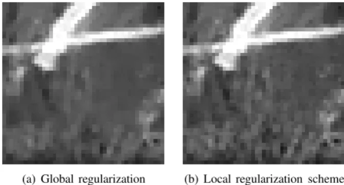
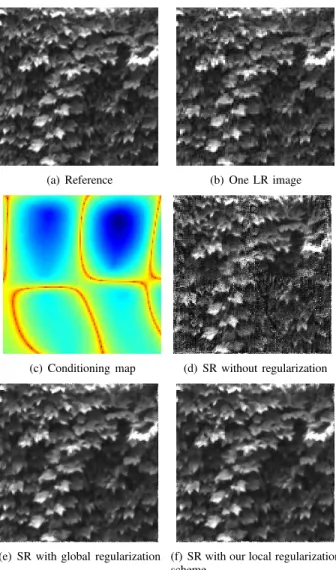
On the other hand, for reconstructing the frequency spectrum or the time signal of prelocalized sources, the regularization term has to reflect prior information on the nature of

The underlying idea behind this regularization strategy was to combine the advantages of the iterated Tikhonov regularization, which can be thought as an iterative refinement of

In particular, the practical interest of updating the regularization parameter during the identification process has been pointed out, as well as the relative performances of

It is expected that the result is not true with = 0 as soon as the degree of α is ≥ 3, which means that it is expected no real algebraic number of degree at least 3 is

A distribution-wise GP model is a model with improved interpolation properties at redundant points: the trajectories pass through data points that are uniquely defined

It can be seen as an extension to the space-time domain of the Proper Generalized Decomposition (PGD) method previously proposed in DIC [6] where the dimensions of space were

First introduced by Faddeev and Kashaev [7, 9], the quantum dilogarithm G b (x) and its variants S b (x) and g b (x) play a crucial role in the study of positive representations

[r]