State-of-the-art on Current Formalisms used in Cyber-Physical Systems Development

(1)

HAL Id: hal-03168832

https://hal.archives-ouvertes.fr/hal-03168832

Submitted on 14 Mar 2021

HAL is a multi-disciplinary open access archive for the deposit and dissemination of sci-entific research documents, whether they are pub-lished or not. The documents may come from teaching and research institutions in France or abroad, or from public or private research centers.

L’archive ouverte pluridisciplinaire HAL, est destinée au dépôt et à la diffusion de documents scientifiques de niveau recherche, publiés ou non, émanant des établissements d’enseignement et de recherche français ou étrangers, des laboratoires publics ou privés.

Cyber-Physical Systems Development

Stefan Klikovits, Rima Al-Ali, Moussa Amrani, Ankica Barisic, Fernando

Barros, Dominique Blouin, Etienne Borde, Didier Buchs, Holger Giese, Miguel

Goulão, et al.

To cite this version:

Stefan Klikovits, Rima Al-Ali, Moussa Amrani, Ankica Barisic, Fernando Barros, et al.. State-of-the-art on Current Formalisms used in Cyber-Physical Systems Development. [Research Report] COST European Cooperation in Science and Technology. 2019. �hal-03168832�

(2)

State-of-the-art on Current Formalisms

used in Cyber-Physical Systems

Development

Stefan Klikovits, Rima Al-Ali, Moussa Amrani, Ankica Bariši´c, Fernando

Barros, Dominique Blouin, Etienne Borde, Didier Buchs, Holger Giese,

Miguel Goulão, Mauro Iacono, Florin Leon, Eva Navarro, Patrizio

Pelliccione, Ken Vanherpen

Deliverable: WG1.1

Core Team Document Info

University of Antwerp, Belgium Deliverable WG1.1 New University of Lisbon, Portugal Dissemination Restricted Telecom ParisTech, Paris, France Status Final

Hasso-Plattner Inst., Potsdam, Germany Doc’s Lead Partner Hasso-Plattner Inst. University of Geneva, Switzerland Date January 7, 2019 Charles University, Prague, Czech Republic Version 3.0

University of Manchester, UK Pages 86 University of Coimbra, Portugal

University of Namur, Belgium

University of Campania Luigi Vanvitelli, Caserta, Italy Technical University Asachi of Iasi, Romania

(3)

(4)

1 Introduction 1 2 Structured Catalog of Modelling Languages and Tools 3

2.1 Catalog Structure . . . 4

2.2 Formalisms . . . 5

2.3 Languages . . . 22

2.4 Tools . . . 49

3 Summary and Future Work 70

Bibliography 71

(5)

(6)

This report presents a substantial catalog of formalisms, modelling languages and tools that are used in the domain of cyber-physical systems modelling. It is part of the deliverable produced by the MPM4CPS’s1Working Group 1 (WG1) on Foundations of MPM4CPS.

Initial WG1 developments prompted the use of ontologies for the analysis of structures and relations of modelling elements. In particular, ontlologies are well supported by the OWL for-malism and its Protege tool, which allowed to formally capture these modeling elements and their relationships, and to reason about them. Such domain analysis allowed to derive a classi-fication that served as the backbone structure of this catalog.

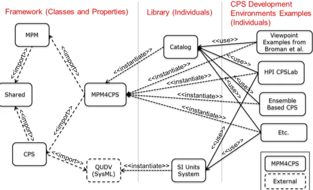
Figure 1.1: Overview of the structure of the MPM4CPS ontology

In particular, figure 1.1 provides an overview of the MPM4CPS ontology (shown in the first col-umn). It emphasises the unification of the two domains of Multi-Paradigm Modelling (MPM) and Cyber-Physical Systems (CPS), which are both foundations for this new emerging domain. The figure further shows that the catalog (i.e. the contents of this document) is an instanti-ation of the MPM4CPS domain. The right column of the figure shows few examples of CPS developments that use multi-paradigm modelling. These examples will not be presented in this report, but are elaborated on in the Framework to Relate / Combine Modeling Languages

and Techniques (see Deliverable D1.2 Giese and Blouin (2016)).

Automatic Catalog Creation: As stated, the individual formalisms, languages and tools of this

catalog are based upon the MPM4CPS ontology. As one can easily imagine, many of the over 170 individual representatives of these concepts contain numerous connections to other indi-viduals. In general, a tight network of dependencies, compatibilities and other relations was discovered. To fully exploit modern technologies, the catalog entries were entered directly into the ontology, so that the connections could be defined. This catalog is generated directly from these ontology sources and thus shows one view of this ontology. As an interactive, searchable

(7)

and visual depiction of this data provides a more comprehensive view than this static genera-tion, we are in the process of publishing the digital ontology alongside the final report.

Usage of this catalog This catalog serves as a valuable source of information and can be used

as a reference to look up data about a large number of current modelling technologies and approaches. The authors tried to add further references to each entry, such that formalisms show scientific references or sources of introduction material, and tool implementations are annotated with a hyperlink to the tool’s webpage, where it can be downloaded from.

The catalog is structured as follows: Chapter 2 presents the list of identified formalisms (Sec-tion 2.2), modelling languages (Sec(Sec-tion 2.3) and modelling tools (Sec(Sec-tion 2.4). The list items each have a short description, extended by references and links to further resources to guide interested readers towards further information.

(8)

The MPM4CPS domain merges concepts from multi-paradigm modelling (MPM) and applies them onto the development of cyber-physical systems. As an extension of the well-known field of embedded systems development, the CPS discipline emerges from a widely studied field and thus builds upon its previous insights, development and modelling approaches and languages and tools.

On the other hand, CPS is a very recent field that embraces new ideas and modern paradigms. These additions created diverging branches from existing standards and new target audiences and domain actors adopted multiple approaches: the result is that different stakeholders use different definitions for their approaches, with an evident dispersion of effort and a significant introduction of unnecessary conceptual entropy in the field in both literature and practice, that may be dominated by a substanding unifying approach suitable to keep beneficial diversity. Consequently, MPM’s aim is to further the diversity of topics by taking a very elastic approach and supporting generic (informal) definitions and merging the “best formalisms, languages and tools” for each point of view. This stance however resulted in the creation of tools that were generated based on different needs and from different points of view, spanning from small-scale, theoretical and hardware-centric approaches to robust, practical, industrial and large-scale applications, and numerous other solutions inbetween.

This chaotic richness of tools is further founded by the heterogeneity of users and backgrounds that are involved in the MPM4CPS processes. MPM4CPS processes mirror the intrinsic com-plexity of their systems and diversity of their users. These come from and work in different do-mains, each bringing their specialised point of view, heritage and methods of their respective domain. Such methods belong to different phases of the design, development and assessment cycle, and stem from various research fields, with particular perspectives on the same problems and different views on similar systems. As a result, specifications of tools are often divergent, even if not contrasting, as they are driven by different purposes, towards different goals, and on different methodological foundations.

This catalog aims to serve as a small collection of the most commonly employed tools, mod-elling languages and formalisms in the domain. The catalog’s initial purpose prescribed to cap-ture current and actively used means to model CPS. However, it quickly became evident that the domain’s vastness cannot be captured entirely in this document. Too many tools and lan-guages have been developed and trialed in many experiments and evaluated on numerous case studies. Instead, the decision was made to initially create a description of the most commonly known and used representatives of each category, and, in a second iteration, add representative usage reports and evaluations.

The catalog is by no means attempting to be complete or even exhaustive, as the described vastness and the speed of development, adaptation and change of the discipline renders such a goal unreachable. What it does however is to serve as a reference for newcomers who wish to learn more about a particular formalism, language or tool. The catalog further provides references to additional information resources such as experience reports, case studies and analyses.

Catalog entries has been selected by experts in their respective fields and participants of the MPM4CPS’s WG1 on Foundations. Collectively, they serve as a current snapshot of the main and most important concepts, but – similar to other lexica and reference sources – has to be extended, revisited and updated in regular intervals (as intended by the members of WG1).

(9)

2.1 Catalog Structure

The structure of the catalog is inspired by the framework proposed by Broman et al. (2012), which distinguishes between viewpoints, formalisms, and languages and tools. It defines that stakeholders have viewpoints which are expressed using formalisms. As formalisms are mathe-matical structures (i.e. without a concrete syntax), they require languages and tools that imple-ment them. Figure 2.1 depicts this framework visually. Evidently, modern tools often support several languages, and each language can merge several formalisms. For example, Papyrus is a tool that supports the creation of different Unified Modeling Language (UML) diagram types such as class diagrams, sequence diagrams, etc. Each diagram is based upon a different formal-ism.

Figure 2.1: Framework for Viewpoints, Formalisms, Languages and Tools (from Broman et al. (2012))

The catalog lists its entries in a pre-defined order, starting from the most theoretical (for-malisms) to the most practical (tools). In some situations, the classification of individual en-tries is not easily possible. For example, Petri nets are a family of formalisms that are well-suited for the expression of concurrency. There are various “flavours” of Petri nets that allow the ex-pression of different systems. As they are closely related though, the catalog authors choose to list them as individual formalisms, even though one might argue that Colored Petri nets are a formalism by themselves. Another issue arises with the classification of Petri nets, as, when they were introduced, Petri nets were equipped with a visual notation syntax, which nowadays is used interchangeably with the mathematical formalism. This catalog thus lists two different entries for “Petri nets” (i.e. the formalism) and “Petri nets diagram” (i.e. its graphical syntax). The reason behind this is that there exists for example the PNML (Petri Net Markup Language) format, which is a common exchange format for Petri net diagrams that can be easily read and written by tools. It is thus another language (with a concrete, textual syntax) for the Petri nets formalism. Finally, the tools section (Section 2.4) provides a list of tools that can be used to cre-ate, edit, and interact with models. For example, the section contains an entry for StrataGEM, a common tool for the model-checking of concurrent models such as Petri nets.

(10)

2.2 Formalisms

The following subsections present the most commonly used formalisms for cyber-physical sys-tems development.

2.2.1 Automata-based Formalisms 2.2.1.1 Abstract State Machines

Abstract state machines are a formalism that model the states and their transitions. ASM are an extension of Finite State Machines (FSM) and allow the representation of states as arbitrary data types. The formalism aims to bridge the gap between human-readable, easily understand-able specifications and machine-executunderstand-able code. Application areas of ASM are for example the modelling and verification of programming languages, protocols, embedded systems, etc.

Implementing Languages

Abstract State Machines is a formalism for the following languages: • AADL (see section 2.3.3)

• AsmL (see section 2.3.9) • AsmetaL (see section 2.3.8) • Gofer (see section 2.3.21)

References

• Börger, E. and W. Schulte (1999), A Programmer Friendly Modular Definition of the

Seman-tics of Java, Springer Berlin Heidelberg, Berlin, Heidelberg, pp. 353–404, ISBN

978-3-540-48737-1, doi: 10.1007/3-540-48737-9_10.

https://doi.org/10.1007/3-540-48737-9_10

• Borger, E. (2005), Abstract state machines and high-level system design and analysis,

The-oretical Computer Science, 336, 2, pp. 205 – 207, ISSN 0304-3975

• Börger, E. and R. Stärk (2003), Springer Berlin Heidelberg, Berlin, Heidelberg.

https://doi.org/10.1007/978-3-642-18216-7

2.2.1.2 Cellular Automata

Cellular Automata (CA) is a popular formalism for the idealisation of physical systems. A sys-tem consists of an n-dimensional lattice of uniform “cells”. Each cell is an automaton, whose behaviour (discrete state transitions) is defined by its own state, and the states of cells in its “neighbourhood” (the cells with a certain distance, e.g. direct neighbours). The transitions of all CA in the system are executed at the same time. By representing automaton behaviour using relatively simple rules, highly complex system behaviour can be expressed. Since their introduction in the 1950ies, cellular automata had various waves of popularity. Recently they are used to model and study emergent behaviour in very large and highly complex systems consisting of uniform units. One of the most popular CA case studies is Conway’s “Game of Life”.

None

References

• Chopard, B. (2012), Cellular Automata Modeling of Physical Systems, Springer New York, New York, NY, pp. 407–433, ISBN 978-1-4614-1800-9, doi: 10.1007/978-1-4614-1800-9_27.

(11)

• (2018), Cellular-Automata Website, https://plato.stanford.edu/entries/ cellular-automata/

• Athanassopoulos, S., C. Kaklamanis, G. Kalfountzos and E. Papaioannou (2012), Cellular Automata for Topology Control in Wireless Sensor Networks Using Matlab, in Proceedings

of the 44th IEEE Conference on Decision and Control, volume 164, volume 164

2.2.1.3 Hybrid Automata-based Formalisms 2.2.1.4 Hybrid Automata

A finite state automaton is a computational abstraction of the transitions of a system between discrete states or locations (on and off, for instance). A hybrid automaton, additionally, consid-ers dynamical evolution over time in each location. This dynamical evolution is represented by a dynamical system. Depending on the nature of the dynamics of this system, different types of hybrid automata are defined; the main ones are explained as follows. Hybrid automata is one of the many existing modelling frameworks of hybrid systems.

Hybrid Automata is a formalism for the following languages: • Stateflow Language (see section 2.3.64)

• Scilab Language (see section 2.3.54) • PyDSTool Language (see section 2.3.50) • NuSMV Language (see section 2.3.36) • Ptolemy Language (see section 2.3.49) • Modelica (see section 2.3.32)

References

• Lygeros, J. and M. Prandini (2010), Stochastic Hybrid Systems: A Powerful Framework for Complex, Large Scale Applications, European Journal of Control, 16, 6, pp. 583 – 594, ISSN 0947-3580, doi: https://doi.org/10.3166/ejc.16.583-594.

http://www.sciencedirect.com/science/article/pii/S0947358010706889

• Abate, A., J.-P. Katoen, J. Lygeros and M. Prandini (2010), Approximate Model Checking of Stochastic Hybrid Systems, European Journal of Control, 16, 6, pp. 624 – 641, ISSN 0947-3580, doi: https://doi.org/10.3166/ejc.16.624-641.

2.2.1.5 I/O Hybrid Automata (Hybrid Input/Output Automata)

I/O hybrid automata are a class of hybrid automata that include asynchronous distributed sys-tem components. The automaton’s transitions are annotated with input actions and output actions, which are executed at when triggering a transition.

None

References

• Lynch, N. A. and M. R. Tuttle (1989), An introduction to input/output automata, CWI

Quarterly, 2, pp. 219–246

• Lynch, N., R. Segala and F. Vaandrager (2003), Hybrid I/O automata, Information and

(12)

https://doi.org/10.1016/S0890-5401(03)00067-1.

2.2.1.6 Linear Hybrid Automata

A linear hybrid automaton is a hybrid automaton where the dynamical system within each location or discrete state is linear.

Linear Hybrid Automata is a formalism for the following languages: • Stateflow Language (see section 2.3.64)

References

2.2.1.7 Non-Linear Hybrid Automata

A nonlinear hybrid automaton is a hybrid automaton where the dynamical system within each location or discrete state is nonlinear. The studies on nonlinear hybrid automata are much less than in linear hybrid automata due to the complexity of the dynamical behaviours involved.

Non-Linear Hybrid Automata is a formalism for the following languages: • Stateflow Language (see section 2.3.64)

References

(13)

2.2.1.8 PTAs (Priced/Probabilistic Timed Automata)

A priced timed automaton is a timed automaton where transitions and locations are annotated with real-valued costs and cost rates, respectively. The global cost increases according to the cost rate of the current location and “jumps” when taking a transition (according to the cost annotation of the transition).

Note, that the cost rate of each location can be different, but cannot be negative.

PTAs is a formalism for the following languages: • PRISM Language (see section 2.3.44)

References

• Behrmann, G., K. G. Larsen and J. I. Rasmussen (2005), Priced Timed Automata: Al-gorithms and Applications, in Formal Methods for Components and Objects, Eds. F. S. de Boer, M. M. Bonsangue, S. Graf and W.-P. de Roever, Springer Berlin Heidelberg, Berlin, Heidelberg, pp. 162–182, ISBN 978-3-540-31939-9

2.2.1.9 Stochastic Hybrid Automata

A stochastic hybrid automaton is a class of non-deterministic hybrid automaton where uncer-tainty is introduced in the system evolution and the control inputs. The main differences with respect to a hybrid automaton are: 1) the initial state (initial discrete location and initial con-tinuous state vector) is chosen at random, 2) the concon-tinuous state evolves following stochastic differential equations, 3) there are two types of discrete transitions between locations that give rise to two types of guards conditions: forced transitions and spontaneous transitions; sponta-neous transitions are triggered by stochastic events.

Stochastic Hybrid Automata is a formalism for the following languages: • Stateflow Language (see section 2.3.64)

• Scilab Language (see section 2.3.54) • PyDSTool Language (see section 2.3.50) • Simulink Language (see section 2.3.59) • Ptolemy Language (see section 2.3.49) • Modelica (see section 2.3.32)

References

• Abate, A., J.-P. Katoen, J. Lygeros and M. Prandini (2010), Approximate Model Checking of Stochastic Hybrid Systems, European Journal of Control, 16, 6, pp. 624 – 641, ISSN

(14)

0947-3580, doi: https://doi.org/10.3166/ejc.16.624-641.

2.2.1.10 Stochastic Timed Automata

Stochastic timed automata extend the TA formalism by adding probabilistic concepts, which allow the stochastic selection of enabled transitions and delays (i.e. time spent within a loca-tion).

Stochastic Timed Automata is a formalism for the following languages: • UPPAAL SMC Language (see section 2.3.72)

References

• Bertrand, N., P. Bouyer, T. Brihaye, Q. Menet, C. Baier, M. Groesser and M. Jurdzinski (2014), Stochastic timed automata, Logical Methods in Computer Science, 10, 4, p. 73, doi: 10.2168/LMCS-10(4:6)2014.

https://hal.inria.fr/hal-01102368

2.2.1.11 Timed Automata

Timed automata (TA) is a formalism that merges the concepts of discrete automata theory with the continuous evolution of variables (“clocks”). Each clock progressively increases its value at a constant rate (i.e. 1). Transition guards can be defined by comparing the clocks’ values to constants. Further, each clock can be reset to zero when firing transitions.

Timed automata can be seen as a specialisation of hybrid automata, where all clock rates are constant and equal, transition guards only allow linear comparisons of clocks and transitions (hybrid automata jumps) can only reset clock values to zero.

Many extensions of timed automata have been proposed, such as stopwatch automata (the rate can be temporarily set to 0), and hourglass automata (the clocks’ rate can be reversed to -1).

Timed Automata is a formalism for the following languages: • HyTech Language (see section 2.3.22)

• Kronos Language (see section 2.3.26) • UPPAAL Language (see section 2.3.71)

References

• Alur, R. and D. L. Dill (1994), A Theory of Timed Automata, Theor. Comput. Sci., 126, 2, pp. 183–235, ISSN 0304-3975, doi: 10.1016/0304-3975(94)90010-8.

http://dx.doi.org/10.1016/0304-3975(94)90010-8

• Cassez, F. and K. Larsen (2000), The Impressive Power of Stopwatches, in International

Conference on Concurrency Theory, Springer, pp. 138–152

• Bengtsson, J. and W. Yi (2004), Timed Automata: Semantics, Algorithms and Tools, Springer Berlin Heidelberg, Berlin, Heidelberg, pp. 87–124, ISBN 978-3-540-27755-2, doi: 10.1007/ 978-3-540-27755-2_3.

https://doi.org/10.1007/978-3-540-27755-2_3

• Osada, Y., T. French, M. Reynolds and H. Smallbone (2014), Hourglass Automata,

Elec-tronic Proceedings in Theoretical Computer Science, 161, pp. 175–188, ISSN 2075-2180,

(15)

2.2.1.12 Timed I/O Automata (Timed Input/Output Automata)

The Timed I/O Automata formalism is an extension of interface automata to include timing information. The automaton’s transitions are annotated with input actions and output actions, which are executed at when triggering a transition.

None

References

• Kaynar, D. K., N. Lynch, R. Segala and F. Vaandrager (2010), The theory of timed I/O au-tomata, Synthesis Lectures on Distributed Computing Theory, 1, 1, pp. 1–137

• David, A., K. G. Larsen, A. Legay, U. Nyman and A. Wasowski (2010), Timed I/O Automata: A Complete Specification Theory for Real-time Systems, in Proceedings of the 13th ACM

International Conference on Hybrid Systems: Computation and Control, ACM, New York,

NY, USA, HSCC ’10, pp. 91–100, ISBN 978-1-60558-955-8, doi: 10.1145/1755952.1755967.

http://doi.acm.org/10.1145/1755952.1755967

2.2.2 Flow-based Formalisms 2.2.2.1 Data Flow

DataFlow describes an computation model that resembles a graph. Each node represents a function (usually called actor) and each arc represents a communication channel between two functions. All the inputs of a function must be present to start its execution. In synchronous dataflow modelling the “synchronous hypothesis” states that the computation of each function and the communication between two functions is infinitely fast (or instantaneous).

Given this hypothesis, SDF provides a sound model of computation with predictable perfor-mance, properties verification methods (liveness, deadlock freedom), and predictable buffer-ing.

The practical approach relies on the fact that the computation of a node starts only when the execution of all its predecessors is finished. This requires that the graph topology is loop-free. Since SDF are usually executed in periodic tasks, the synchronous hypothesis is usually con-sidered to be verified as the worst case response time of the graph is smaller than the task’s period.

This type of model is well-suited to digital signal processing and communications systems which often process an endless supply of data. It has been successfully applied in the domain of safety critical embedded systems. It has also been characterised or extended into homoge-neous data flow graphs, cyclo-static data flow graphs, scenario-aware data flow graphs, affine data flow graphs.

Data Flow is a formalism for the following languages: • AADL (see section 2.3.3)

• Zélus (see section 2.3.76) • Lustre (see section 2.3.28) • Signal (see section 2.3.55)

(16)

• Murthy, P. K. and E. A. Lee (2002), Multidimensional synchronous dataflow, IEEE

Transac-tions on Signal Processing, 50, 8, pp. 2064–2079, ISSN 1053-587X, doi: 10.1109/TSP.2002.

800830

2.2.2.2 HyFlow (Hybrid Flow System Specification)

HyFlow provides a formal description of dynamic topology hybrid systems Barros (2003). This formalism can model systems that exhibit both continuous and discrete behaviors while re-lying on a digital computer representation. HyFlow supports multisampling as a first order operator, enabling both time and component varying sampling, making it suitable for repre-senting sampled-based systems, like digital controllers and filters. HyFlow provides also an extrapolation operator that enables an error free representation of continuous signals. Multi-sampling can be used for achieving an explicit representation of asynchronous adaptive step-size differential equations integrators Barros (2018). HyFlow provides an integrative framework for combing models expressed in different modeling paradigms. In particular, fluid stochastic Petri-nets Barros (2015) and geometric integrators Barros (2018), for example, can be repre-sented in the HyFlow formalism, enabling its seamless integration with other HyFlow mod-els. HyFlow sampling provides an expressive operator for making the connection of computer-based systems with real-time systems, since sampling is, in many cases, the most convenient operator to interact with continuous signals. HyFlow supports modular and hierarchical mod-els providing deterministic semantics for model composition and co-simulation Barros (2008).

None

References

• Barros, F. J. (2018), Modular representation of asynchronous geometric integrators with support for dynamic topology, SIMULATION, 94, 3, pp. 259–274

• Barros, F. J. (2008), Semantics of Dynamic Structure Event-based Systems, in Proceedings

of the Second International Conference on Distributed Event-based Systems, ACM, New

York, NY, USA, DEBS ’08, pp. 245–252, ISBN 978-1-60558-090-6, doi: 10.1145/1385989. 1386020.

http://doi.acm.org/10.1145/1385989.1386020

• Barros, F. J. (2003), Dynamic Structure Multiparadigm Modeling and Simulation, ACM

Trans. Model. Comput. Simul., 13, 3, pp. 259–275, ISSN 1049-3301, doi: 10.1145/937332.

937335.

http://doi.acm.org/10.1145/937332.937335

• Barros, F. (2015), A Modular Representation of Fluid Stochastic Petri Nets, in Symposium

on Theory of Modeling and Simulation

2.2.3 Logic-based Formalisms

2.2.3.1 CTL (Computation Tree Logic)

CTL is a branching-time temporal logic that allows the analysis of tree-like structures. It allows the analysis of various future evolution paths to answer questions whether there is a possibility that an event might or will happen. Various model checkers exist that allow the verification of the reachability and liveness of certain events (or event sequences).

CTL is a formalism for the following languages: • NuSMV Language (see section 2.3.36)

(17)

References

• Huth, M. and M. Ryan (2004), Logic in Computer Science: Modelling and Reasoning about

Systems, Cambridge University Press, 2 edition, doi: 10.1017/CBO9780511810275

2.2.3.2 First Order Logic

First-Order Logic (FOL, also “First-Order Predicate Calculus”) is a logical formalism constituted of terms and formulas. A term is either a variable, a function symbol or a predicate symbol. A formula is constituted of formulas built over terms combined with the usual Boolean operators (negation, conjunction and so on) and both existential and universal quantifiers. First-Order Logic formulas are interpreted on a (finite) domain, and possess a sound and complete calcu-lus, making it automatable for reasoning Kleene (2002).

First Order Logic is a formalism for the following languages: • SMT-LIB (see section 2.3.61)

References

• Kleene, S. C. (2002), Mathematical Logic, Wiley

2.2.3.3 Linear Temporal Logic

LTL is a representative of the family of temporal logics that analyses the future evolution of paths. It allows the testing of one individual branch (as opposed to CTL).

Linear Temporal Logic is a formalism for the following languages: • Kronos Language (see section 2.3.26)

• PSC (see section 2.3.47)

References

• Huth, M. and M. Dermot Ryan (2000), Logic in computer science - modelling and reasoning

about systems., ISBN 978-0-521-65602-3

2.2.3.4 Temporal Logic

A temporal logic (also tense logic) system is a formal mathematical system that allows the rea-soning about terms and their truth value related to time. It is an extension of first-order logic and allows the expression of statements such as "I always model CPS", "I will eventually model a CPS’" and "I will not model CPS until I find a good formalism".

Temporal logic is frequently used in formal verification, where it is used to formally express requirements (e.g. the reaching of a certain state). Popular temporal logic systems are for ex-ample the linear temporal logic (LTL), computation tree logic (CTL) and Hennessy-Milner logic (HML).

Temporal Logic is a formalism for the following languages: • NuSMV Language (see section 2.3.36)

References

• Pnueli, A. (1977), The Temporal Logic of Programs, in Proceedings of the 18th Annual

(18)

USA, SFCS ’77, pp. 46–57, doi: 10.1109/SFCS.1977.32.

https://doi.org/10.1109/SFCS.1977.32

2.2.4 Petri Net-based Formalisms 2.2.4.1 High Level Petri Nets

This large class rely on another modeling framework devoted to the description of the data attached to the tokens, and the expression that must be assigned to arcs describing the com-putation that must be done for satisfying the pre and post conditions. Among several dialect of these class we can cite algebraic Petri Nets and coloured Petri Nets.

High Level Petri Nets is a formalism for the following languages: • PNML (see section 2.3.43)

• Petri Net Diagram (see section 2.3.42)

References

2.2.4.2 Petri Net (Place Transition Nets)

A Petri net (also known as a place/transition net or P/T net) is a formalism for the description of dynamic discrete systems. It is particularly suited to the modeling of systems where distribu-tion, concurrency and non-determinism is important to discribe and analyze. The mathemat-ical foundation of Petri nets has led to several development to make possible complex analsis of systems decribed by Petri nets. A Petri net is a directed bipartite graph, in which the nodes represent transitions (i.e. events that may occur, represented by bars or black rectangles) and places (i.e. conditions or ressources, represented by circles). The directed arcs describe which places are pre- and/or postconditions for which transitions (signified by arrows). Petri nets were invented, according to some sources, in August 1939 by Carl Adam Petri at the age of 13 for the purpose of describing chemical processes.

Petri nets offer a graphical notation which is of particular interest to the engineer analyzing sys-tems, natural pattern of design are existing in Petri nets such as causality, choice, independence and ressource management.

There are attempts for several formalisms Like UML activity diagrams, Business Process Model and Notation and EPCs to have semantics in term of translation into Petri nets. These transla-tions have been used to provide a precise semantics to such formalisms as well as to develop tools for their simulation and analysis.

It has been observed that in practice Petri Nets lack of modeling power for some modeling dimensions such as: timing aspects, data structures, stochastic processes and event priority. In general the formal analysis tool need different techniques if new modeling dimensions are introduced. So tools are generally different and adapted to the specific extensions.

Petri Nets have several extensions which are concretised in the following formalisms, it must be noted that the computing power of such extensions can change according to the new concepts introduced in the notations (i.e. time) and then the analysability of the models is sometime much more difficult or limited to extention with finiteness assumptions (i.e. high level nets):

Petri Net is a formalism for the following languages: • PNML (see section 2.3.43)

(19)

• FIACRE (see section 2.3.18)

References

• CPN preserve useful properties of Petri nets and at the same time extend initial formalism to allow the distinction between tokens. Coloured Petri Nets allow tokens to have a data value attached to them. This attached data value is called token color.

https://en.wikipedia.org/wiki/Coloured_Petri_net

2.2.4.3 Petri Nets with Priority

This simple extension bring new semantics to the transition firing in order to solve conflict. Depending on the variant it can lead to more powerful models which are Turing complete.

Petri Nets with Priority is a formalism for the following languages: • PNML (see section 2.3.43)

References

2.2.4.4 Stochastic Petri Nets

The firing of transitions follows a probabilistic distibution on time duration or frequency of transitions firing when there is a conflict.

Stochastic Petri Nets is a formalism for the following languages: • PNML (see section 2.3.43)

References

2.2.4.5 Timed Petri Nets

Timed Petri Nets introduce time as a modeling dimension. This is reflected in aspect such as transition duration or possible interval for firing transitions. Generally these classes bring new problems for analysing them, in particular the time-line which has no limit in the future and the density of the time.

Timed Petri Nets is a formalism for the following languages: • PNML (see section 2.3.43)

• Petri Net Diagram (see section 2.3.42) • FIACRE (see section 2.3.18)

References

• Abdulla, P. A. and A. Nylén (2001), Timed Petri Nets and BQOs, in Applications and Theory

of Petri Nets 2001, Eds. J.-M. Colom and M. Koutny, Springer Berlin Heidelberg, Berlin,

Heidelberg, pp. 53–70, ISBN 978-3-540-45740-4

• Berthomieu, B. and M. Diaz (1991), Modeling and verification of time dependent systems using time Petri nets, IEEE Transactions on Software Engineering, 17, 3, pp. 259–273, ISSN 0098-5589, doi: 10.1109/32.75415

(20)

2.2.5 Other Formalisms 2.2.5.1 Bayesian Networks

Bayesian networks are a formalism that establishes a probabilistic graph model. The ver-tices of the directed acyclic graph represent random variable probabilities and edges between them represent probabilistic dependencies. Hence each vertex depends on its predecessors. Bayesian networks are well-suited to create simple computations for models with many vari-ables. They can further be used to encode hypotheses, hypotheses, beliefs, and latent varivari-ables.

None

References

• Niedermayer, D. (2008), An Introduction to Bayesian Networks and Their Contemporary

Applications, Springer Berlin Heidelberg, Berlin, Heidelberg, pp. 117–130, ISBN

978-3-540-85066-3, doi: 10.1007/978-3-540-85066-3_5.

https://doi.org/10.1007/978-3-540-85066-3_5

2.2.5.2 Bond Graphs

Bond graphs focus on the modelling of energy flows. The formalism recognises that different energy domains (electrical, hydraulic, mechanical) can be similarly represented and that the dual forces of "flow" (e.g. current, velocity) and “effort” (e.g. voltage, force) in combination cre-ate power. Bond graphs models represent idealised energy flows. Usually the same notation is used for all energy domains and domains switches are modelled using e.g. gyrators and trans-formers. The formalism is actively used in engineering domains where it serves good purpose of prototyping the energy flow within a system.

Bond Graphs is a formalism for the following languages: • 20-sim Bond Graph (see section 2.3.2)

References

• Paynter, H. M. (1961), Analysis and Design of Engineering Systems, MIT Press, Cambridge, MA

• Broenink, J. F. (1999), Introduction to Physical Systems Modelling with Bond Graphs, in in

the SiE whitebook on Simulation Methodologies, p. 31

2.2.5.3 Causal Block Diagrams

Causal block diagrams are a visual modelling formalism that connects operation blocks in a graph structure. The graph’s operation block nodes represent computations or transforma-tions of signals, edges model the signals themselves. Typical operation blocks are algebraic functions (e.g. sum, product) but can also represent timed functionality (e.g. delays, integra-tion or derivatives). The formalism is used in many visual modelling tools (e.g. Simulink) and graphical programming languages (e.g. LabVIEW).

Causal Block Diagrams is a formalism for the following languages: • LabVIEW Language (see section 2.3.27)

• Simulink Language (see section 2.3.59)

(21)

• Gomes, C., J. Denil and H. Vangheluwe (2016), Causal-Block Diagrams, Technical report.

http://msdl.cs.mcgill.ca/people/claudio/pub/Gomes2016a.pdf

• Denckla, B. and P. J. Mosterman (2005), Formalizing Causal Block Diagrams for Modeling a Class of Hybrid Dynamic Systems, in Proceedings of the 44th IEEE Conference on Decision

and Control, pp. 4193–4198, ISSN 0191-2216, doi: 10.1109/CDC.2005.1582820

2.2.5.4 Complex Networks

A complex network is a large number of interdependent systems connected in a nontrivial and non-regular manner. The interconnection of these systems produces emergent properties or behaviours which are not present in the isolated systems: this is called self-organisation, col-lective behaviour. There are different representations for complex networks. These models are typically based on graph theory (nodes connected with links). The main models for complex networks are: random-graph networks, small-world networks, scale-free networks. Each of these models have different topological (structural) features, analysed with tools from statisti-cal physics.

Complex Networks is a formalism for the following languages: • Visone Language (see section 2.3.74)

• Small-World Networks (see section 2.3.60) • NetworkX Language (see section 2.3.35) • Pajek Language (see section 2.3.40)

• Random-Graph Networks (see section 2.3.51) • iGraph Language (see section 2.3.23)

• Mathematica Language (see section 2.3.30) • Cytoscape Language (see section 2.3.13)

• Network Workbench Language (see section 2.3.34)

References

• Navarro-Lopez, E. (2013), DYVERSE: From formal verification to biologically-inspired

real-time self-organizing systems, pp. pp. 301–346, ISBN ISBN-10:1439883270

• H. Strogatz, S. (2001), Exploring Complex Networks, Nature, 410, doi: 10.1038/410268a0.

http://www.nature.com/nature/journal/v410/n6825/pdf/410268a0. pdf

• Barrat, A., M. Barthelemy and A. Vespignani (2008), Dynamical Processes on Complex

Net-works, Cambridge University Press, doi: 10.1017/CBO9780511791383

• Barabási, A.-L. and R. Albert (1999), Emergence of Scaling in Random Networks, Science,

286, 5439, pp. 509–512, ISSN 0036-8075, doi: 10.1126/science.286.5439.509.

http://science.sciencemag.org/content/286/5439/509

• Albert, R. and A.-L. Barabási (2002), Statistical mechanics of complex networks, Rev. Mod.

Phys., 74, pp. 47–97, doi: 10.1103/RevModPhys.74.47.

https://link.aps.org/doi/10.1103/RevModPhys.74.47

• Newman, M. (2003), The Structure and Function of Complex Networks, SIAM Review, 45, 2, pp. 167–256, doi: 10.1137/S003614450342480

(22)

• Wang, X. F. and G. Chen (2003), Complex networks: small-world, scale-free and beyond,

IEEE Circuits and Systems Magazine, 3, 1, pp. 6–20, ISSN 1531-636X, doi: 10.1109/MCAS.

2003.1228503

• Watts, D. and S. H. Strogatz (1998), Collective Dynamics of Small World Networks, Nature,

393, pp. 440–2, doi: 10.1038/30918 2.2.5.5 Differential Equations

Differential equations are frequently used to model the physical phenomena of CPS and in par-ticular the plant of CPSs. They are mathematical equations, consisting of derivatives and func-tions. Differential equations can be classified into ordinary differential equations (ODE), which have a single independent variable, differential-algebraic equations (DAE), which make use of algebraic equations and partial differential equations (PDE), which involve multi-variable functions and partial derivatives.

Differential Equations is a formalism for the following languages: • Zélus (see section 2.3.76)

• Scilab Language (see section 2.3.54) • XPPAUT Language (see section 2.3.75) • PyDSTool Language (see section 2.3.50) • Simulink Language (see section 2.3.59) • Mathematica Language (see section 2.3.30) • Modelica (see section 2.3.32)

References

• Winkel, B. (2016), Nagy, G. 2015. Ordinary Differential Equations.

https://www.simiode.org/resources/2681

2.2.5.6 Discontinuous Systems

Discontinuous or non-smooth systems are a subclass of hybrid systems. There are several types, depending on the type of discontinuity in the model representing the system. Two main classes of discontinuous systems are observable: switching or variable structure systems, and jump or reset systems. Switching or variable structure systems are typically studied through the formalism of sliding motions (dynamics on the discontinuity surface) or sliding-mode-based control systems.

Discontinuous Systems is a formalism for the following languages: • Stateflow Language (see section 2.3.64)

• Scilab Language (see section 2.3.54) • XPPAUT Language (see section 2.3.75) • PyDSTool Language (see section 2.3.50) • Simulink Language (see section 2.3.59) • Ptolemy Language (see section 2.3.49) • Modelica (see section 2.3.32)

(23)

References

• I. Utkin, V. (1992), Sliding Modes in Control Optimization, pp. 12–28, ISBN 978-3-642-84381-5, doi: 10.1007/978-3-642-84379-2_2

• Navarro-Lopez, E. M. (2009a), Hybrid-automaton models for simulating systems with sliding motion: still a challenge, IFAC Proceedings Volumes, 42, 17, pp. 322 – 327, ISSN 1474-6670, doi: https://doi.org/10.3182/20090916-3-ES-3003.00056, 3rd IFAC Confer-ence on Analysis and Design of Hybrid Systems.

• Filippov, A. F. (1990), Differential Equations with Discontinuous Righthand Sides, SIAM

Review, 32, 2, pp. 312–315, doi: 10.1137/1032060. https://doi.org/10.1137/1032060

• Navarro-Lopez, E. M. (2009b), Hybrid modelling of a discontinuous dynamical system including switching control, IFAC Proceedings Volumes, 42, 7, pp. 87 – 92, ISSN 1474-6670, doi: https://doi.org/10.3182/20090622-3-UK-3004.00019, 2nd IFAC Conference on Anal-ysis and Control of Chaotic Systems.

2.2.5.7 Discrete Event

The discrete event (DE) paradigm provides a representation of systems based on piecewise constant state variables. Contrarily to continuous systems, where variables change continu-ously in time, DE systems can only change at a finite number of instants during a finite time interval. The actions causing these changes are commonly called by events. Contrarily to dis-crete time models, where changes are periodic, in DE systems changes can occur randomly, i.e., without any following any periodicity.

Several strategies for organising DE systems have been developed. These descriptions are com-monly termed by world views and provide different organisations for modelling DE systems. Common world views include event scanning Kiviat (1968), activity scanning Buxton and Laski (1962), and process interaction Dahl and Nygaard (1966).

The DEVS formalism Zeigler (1976), provides a formal description of modular DE systems, ab-stracting and unifying many of the concepts required for characterising DE systems. The co-simulation of DE systems was introduced in Zeigler (1984) that has established the separation between models and their simulators, enabling the interoperability of hierarchical and modu-lar DE models.

Discrete Event is a formalism for the following languages: • SIMUL8 Language (see section 2.3.58)

• Simio Language (see section 2.3.57) • ARENA Language (see section 2.3.7) • OMNet++ Language (see section 2.3.39) • MS4 Me Language (see section 2.3.33) • SimEvents Language (see section 2.3.56) • FlexSim Language (see section 2.3.19)

(24)

• Kiviat, P. J. (1968), Introduction to the SIMSCRIPT II Programming Language, in

Proceed-ings of the Second Conference on Applications of Simulations, Winter Simulation

Confer-ence, pp. 32–36.

http://dl.acm.org/citation.cfm?id=800166.805259

• Buxton, J. and J. Laski (1962), Control and Simulation Language, Computer Journal, , 5, pp. 194–199

• Zeigler, B. (1984), Multifaceted Modelling and Discrete Event Simulation, Academic Press, San Diego

• Zeigler, B. (1976), Theory of Modelling and Simulation, Wiley

2.2.5.8 Electrical Linear Networks

Electrical linear networks (ELN) consist of linear electrical components that are interconnected to form a circuit. The electrical components considered are linear, such as: voltage/current sources, resistors, capacitors, inductors and transmission lines. Circuits falling within the ELN category are analysed with well-known linear methods, typically, frequency-domain methods.

Electrical Linear Networks is a formalism for the following languages: • SystemC (see section 2.3.67)

• XPPAUT Language (see section 2.3.75) • PyDSTool Language (see section 2.3.50) • Simulink Language (see section 2.3.59) • SPICE Language (see section 2.3.63)

References

• Banerjee, A. and B. Sur (2014), Electrical Linear Networks in Practice and Theory, Springer International Publishing, Cham, pp. 411–426, ISBN 978-3-319-01147-9, doi: 10.1007/978-3-319-01147-9_15.

https://doi.org/10.1007/978-3-319-01147-9_15

2.2.5.9 Entity Relationship

The entity-relationship model (ER) consists of entity types with relationships that can exist be-tween instances of those types. Originating from the databases domain, ER defines informa-tion structures which can be implemented in a database. Some enhanced ER formalisms also include generalization-specialization relationships so that it can be used for the specification of domain ontologies.

Entity Relationship is a formalism for the following languages: • UML (see section 2.3.69)

• AADL (see section 2.3.3)

• Entity Relationship Diagram (see section 2.3.16) • AUTOSAR Language (see section 2.3.10)

• MetaH (see section 2.3.31) • MARTE (see section 2.3.29)

(25)

References

• Chen, P. P.-S. (2001), The Entity Relationship Model — Toward a Unified View of Data, Springer Berlin Heidelberg, Berlin, Heidelberg, pp. 205–234, ISBN 978-3-642-48354-7, doi: 10.1007/978-3-642-48354-7_7.

https://doi.org/10.1007/978-3-642-48354-7_7

• (2018), Entity Relationship Website, https://www.smartdraw.com/entity-relationship-diagram/

2.2.5.10 Fault Trees

Fault Trees is a formal model designed to analyze and evaluate the origin and the effects of faults in the components of an architecture at its subsystem or system level. The graphs repre-sent the probability of component faults on the edges between nodes, allowing the quick calcu-lation of risks by following the paths of the tree. Many variants have been proposed that extend the basic combinatorial nature of this formalism to include time, repairable components or repairing actions.

None

References

• Ruijters, E. and M. Stoelinga (2015), Fault tree analysis: A survey of the state-of-the-art in modeling, analysis and tools, Computer Science Review, 15-16, pp. 29 – 62, ISSN 1574-0137, doi: https://doi.org/10.1016/j.cosrev.2015.03.001.

2.2.5.11 Markov Chains

Markov chains are a probabilistic model of event sequences. When depicted as graph, each node in a Markov chain represents an event type (e.g. “rolling a die”) and the edges to other nodes represent the outcomes of the event (e.g. the probability of each side). The events need to support the Markov property. This means that predictions on the future evolution of the chain can be made based on the current state, and knowledge of previous evolutions has no influence on this prediction. Markov chains models can be built for discrete events as well as for continuous state space.

Markov Chains is a formalism for the following languages: • PRISM Language (see section 2.3.44)

References

• Sigman, K. (2009), 1 IEOR 6711 : Continuous-Time Markov Chains

• Freedman, D. (1983), Markov chains, Springer-Verlag, New York-Berlin, ISBN 0-387-90808-0, corrected reprint of the 1971 original

2.2.5.12 Process Algebras

Process algebra refer to a group of different calculi that are used to study the evolution of con-current processes and their relations, including communication, synchronisation and interac-tions. Individual processes are seen as agents that continuously interact with each other and the environment. Their well-defined semantics allow for the analysis and verification of highly complex systems. Common process algebras include the Calculus of Communicating Systems

(26)

(CCS), Communicating Sequential Processes (CSP) and the Algebra of Communicating Pro-cesses (ACP).

None

References

• van Glabbeek, R. J. (1987), Bounded nondeterminism and the approximation induction principle in process algebra, in STACS 87, Eds. F. J. Brandenburg, G. Vidal-Naquet and M. Wirsing, Springer Berlin Heidelberg, Berlin, Heidelberg, pp. 336–347, ISBN 978-3-540-47419-7

• Nicola, R. D. (2013), A gentle introduction to Process Algebras

• Fokkink, W. (2000), Introduction to Process Algebra, Springer-Verlag, Berlin, Heidelberg, 1st edition, ISBN 354066579X

2.2.5.13 TFPG (Timed Failure Propagation Graph)

A TFPG model is a relatively simple directed graph structure which identifies the paths along which failures are expected to propagate in the system. Nodes of a TFPG represent failure modes or discrepancies, and arcs represent failure propagation paths with a time interval rep-resenting the lower and upper bound of the failure propagation time. Logical operators AND and OR are used to represent logical combinations of failures to reach a mode and/or a discrep-ancy. TFPG can be used at design time to analyse faults propagation and their consequences. It can also be used at runtime to provide potential explanations to a fault signature that is ob-served during the system execution since consistency checking can be used to eliminate path on which timing constraints are not verified.

None

References

• Ofsthun, S. C. and S. Abdelwahed (2007), Practical applications of timed failure propaga-tion graphs for vehicle diagnosis, in 2007 IEEE Autotestcon, pp. 250–259, ISSN 1088-7725, doi: 10.1109/AUTEST.2007.4374226

• Misra, A. (1999), Robust diagnostic system : structural redundancy approach

• Bozzano, M., A. Cimatti, M. Gario and A. Micheli (2015), SMT-based Validation of Timed Failure Propagation Graphs, in Proceedings of the Twenty-Ninth AAAI Conference on

Arti-ficial Intelligence, AAAI Press, AAAI’15, pp. 3724–3730, ISBN 0-262-51129-0. http://dl.acm.org/citation.cfm?id=2888116.2888233

2.2.5.14 VDM (Vienna Development Method)

VDM is a formal description method for e.g. critical and concurrent systems, and compilers. It was developed in the 1970s and has seen significant industry usage. Its successor version VDM++ extends the modelling language to also support object-oriented systems.

None

References

• Bjørner, D. and C. B. Jones (Eds.) (1978), The Vienna Development Method: The

(27)

2.3 Languages

The following subsections present the most commonly used languages for CPS development.

2.3.1 20-sim Block Diagrams

Block diagrams are a graphical programming and modelling language that is used to model within the 20-sim tool. They are similar to block diagrams in other languages and tools (e.g. Simulink).

Supported Formalisms

20-sim Block Diagrams is based on the following formalisms: • Causal Block Diagrams (see section 2.2.5.3)

Supporting Tools

20-sim Block Diagrams is implemented by the following tools: • 20-sim (see section 2.4.1)

References

• (2018), 20-sim Website,http://20sim.com/

2.3.2 20-sim Bond Graph

Bond graphs model idealized physical processes as graphs and graph networks. The language is implemented in 20-sim and allows the initial modelling of a-causal systems and performing causality analyses.

20-sim Bond Graph is based on the following formalisms: • Bond Graphs (see section 2.2.5.2)

20-sim Bond Graph is implemented by the following tools: • 20-sim (see section 2.4.1)

References

• (2018), 20-sim Website,http://20sim.com/

2.3.3 AADL (Architecture Analysis and Design Language)

The Architecture Design & Analysis Language (AADL) is an architecture description language for the modeling of safety-critical real-time embedded systems. It allows the specification, analysis and code generation of these systems. It is standardized SAE as the As the AS5506C aerospace standard.

AADL allows modeling both the hardware and software parts of a system thus taking into ac-count the deployment of a software application onto an execution platform. Many analysis and code generation tool are provided for AADL.

AADL is extensible and several annex languages have been proposed as described below:

AADL is based on the following formalisms: • Entity Relationship (see section 2.2.5.9)

(28)

• Data Flow (see section 2.2.2.1)

• Abstract State Machines (see section 2.2.1.1)

AADL is implemented by the following tools: • AADL Inspector (see section 2.4.2) • STOOD (see section 2.4.71) • OSATE (see section 2.4.43) • Ocarina (see section 2.4.39) • MASIW (see section 2.4.30) • Polychrony (see section 2.4.49)

References

• (2018b), AADL Website,http://www.aadl.info/

• (2018c), SAE AADL Specification,http://standards.sae.org/as5506b/

2.3.4 ACME

While most Architectural Description Languages (ADLs) considerably overlap on their core fea-tures, each ADL focuses on different aspects of the software architecture and problem cate-gories. The creation of a global ADL would be impractical and developing mappings among each pair of languages would require an excessive amount of effort. Nevertheless, this diver-sity raises difficulties in transferring information among different ADLs. Acme was proposed as common representation of architectural concepts and to support the interchange of informa-tion using a generic language. This reduces the number of required transformainforma-tions to those to and from ACME.

Language Features:

• an architectural ontology consisting of seven basic architectural design elements;

• a flexible annotation mechanism supporting association of non-structural information using externally defined sublanguages;

• a type mechanism for abstracting common, reusable architectural idioms and styles; and • an open semantic framework for reasoning about architectural descriptions.

None

ACME is implemented by the following tools: • ACME Studio (see section 2.4.3)

References

• Garlan, D., R. T. Monroe and D. Wile (2000), Acme: Architectural description of component-based systems, in Foundations of component-based systems, Eds. G. T. Leav-ens and M. Sitaraman, pp. 47–68

• Wile, D. (1996), Semantics for the Architecture Interchange Language, ACME, in Joint

Pro-ceedings of the Second International Software Architecture Workshop (ISAW-2) and Inter-national Workshop on Multiple Perspectives in Software Development (Viewpoints ’96) on

(29)

SIGSOFT ’96 Workshops, ACM, New York, NY, USA, ISAW ’96, pp. 28–30, ISBN

0-89791-867-3, doi: 10.1145/243327.243341.

http://doi.acm.org/10.1145/243327.243341

• Garlan, D., R. Monroe and D. Wile (1997), Acme: An architecture description interchange language, in Proceedings of the 1997 conference of the Centre for Advanced Studies on

Col-laborative research, IBM Press, p. 7

2.3.5 AF3 Language (AutoFOCUS 3 Language)

This is the set of input languages of the AF3 tool.

None

AF3 Language is implemented by the following tools: • AF3 (see section 2.4.4)

References

• (2018), AF3 Website,http://af3.fortiss.org/

2.3.6 Alloy

Alloy is a specification language that allows the description of relations within a model. It is declarative in nature and allows checking of systems for correctness. It is accompanied by a tool implementation, the Alloy Analyzer.

None

Alloy is implemented by the following tools: • Alloy Analyzer (see section 2.4.5)

References

• (2018), Alloy Website,http://alloy.lcs.mit.edu/alloy/

2.3.7 ARENA Language

This is the input anguage of the ARENA simulation tool for discrete events.

ARENA Language is based on the following formalisms: • Discrete Event (see section 2.2.5.7)

ARENA Language is implemented by the following tools: • ARENA (see section 2.4.9)

References

(30)

2.3.8 AsmetaL

AsmetaL is the language used for the creation of models in the Asmeta toolset.

AsmetaL is based on the following formalisms: • Abstract State Machines (see section 2.2.1.1)

AsmetaL is implemented by the following tools: • Asmeta Tools (see section 2.4.10)

References

• (2018a), Asmeta Website,http://asmeta.sourceforge.net/

2.3.9 AsmL (Abstract State Machine Language)

AsmL is a language implementation of the Abstract State Machine (ASM) formalism. It runs on the .NET platform and allows modelling, coding and testing.

AsmL is based on the following formalisms: • Abstract State Machines (see section 2.2.1.1)

None

References

• (2018c), AsmL Website, https://www.microsoft.com/en-us/research/ project/asml-abstract-state-machine-language/

2.3.10 AUTOSAR Language (AUTomotive Open System ARchitecture)

AUTOSAR is a partnership of automotive stakeholders (vehicle manufacturers, suppliers, ser-vice providers and companies) working on establishing an open and standardized software ar-chitecture for automotive electronic control units (ECUs). AUTOSAR includes an arar-chitecture description language for the design of vehicular systems. Application software components are linked through abstract virtual function buses, which represent all hardware and system ser-vices offered by a vehicular system. This allows designers to focus on the application instead of the infrastructure software.

AUTOSAR Language is based on the following formalisms: • Entity Relationship (see section 2.2.5.9)

AUTOSAR Language is implemented by the following tools: • System Desk (see section 2.4.73)

References

(31)

2.3.11 CCSL (Clock Constraint Specification Language)

The CCSL is a language that introduces is the modelling of relations between clocks into the MARTE UML Profile.

None

CCSL is implemented by the following tools: • Time Square (see section 2.4.76)

References

• André, C. and F. Mallet (2008), Clock Constraints in UML/MARTE CCSL, Research Report RR-6540, INRIA.

https://hal.inria.fr/inria-00280941

2.3.12 CDL (Context Description Language)

CDL is a language that uses UML Activity and Sequence diagrams to model a system’s context and environment. It is implemented in OBP toolset, which allows properties to be checked.

None

CDL is implemented by the following tools: • OBP Explorer (see section 2.4.38) • TINA (see section 2.4.77)

References

• Dhaussy, P., J. Auvray, S. de Belloy, F. Boniol and E. Landel (2008), Using context descrip-tions and property definition patterns for software formal verification, in 2008 IEEE

Inter-national Conference on Software Testing Verification and Validation Workshop, pp. 89–96,

doi: 10.1109/ICSTW.2008.52

• (2018), OBPCDL Website,http://www.obpcdl.org/

2.3.13 Cytoscape Language

This is the input language of the Cytoscape tool for biological networks.

Cytoscape Language is based on the following formalisms: • Complex Networks (see section 2.2.5.4)

Cytoscape Language is implemented by the following tools: • Cytoscape (see section 2.4.16)

References

(32)

2.3.14 DEECo (Dependable Emergent Ensembles of Component)

DEECo is an architecture description language with a computational model that is used to de-sign autonomous components. It is part of ASCENS project. More specifically, it captures the self-adaptation in the components and implicit exchanging of information in a dynamically formed group of components (i.e. ensemble). The formation of the ensemble is impacted by changes in the environment. The concepts presented in this computational model follows SCEL (see section 2.3.53) That is based on (see section 2.3.53).

From implementation perspective, the user uses java and follows a specific structure in writing the components and the ensembles, which conceptually matches the DSL presented in the papers. Multiple java annotations are employed to capture the structure.

None

DEECo is implemented by the following tools: • jDEECo (see section 2.4.26)

References

• Bures, T., I. Gerostathopoulos, P. Hnetynka, J. Keznikl, M. Kit and F. Plasil (2013), DEECO: An Ensemble-based Component System, in Proceedings of the 16th International ACM

Sigsoft Symposium on Component-based Software Engineering, ACM, New York, NY, USA,

CBSE ’13, pp. 81–90, ISBN 978-1-4503-2122-8, doi: 10.1145/2465449.2465462.

http://doi.acm.org/10.1145/2465449.2465462

• Keznikl, J., T. Bures, F. Plasil and M. Kit (2012), Towards Dependable Emergent Ensembles of Components: The DEECo Component Model, in 2012 Joint Working IEEE/IFIP

Con-ference on Software Architecture and European ConCon-ference on Software Architecture, pp.

249–252, doi: 10.1109/WICSA-ECSA.212.39 •

•

2.3.15 EAST-ADL

EAST-ADL is an ADL for the automotive embedded domain. It ties concepts from UML, SysML and AADL to the AUTOSAR environment.

None

EAST-ADL is implemented by the following tools: • Papyrus (see section 2.4.47)

References

• (2018), EAST-ADL Website,http://www.east-adl.info

2.3.16 Entity Relationship Diagram

Entity relationship diagrams are a visual, graphical modelling language for specifying relations within a domain. The language is primarily used to create models of relational databases.

(33)

Entity Relationship Diagram is based on the following formalisms: • Entity Relationship (see section 2.2.5.9)

None

References

• (2018), Entity Relationship Website, https://www.smartdraw.com/entity-relationship-diagram/

2.3.17 FCM (Flex-eWare Component Model)

FCM is an extension of the CORBA Component Model (CCM) in the aim of providing a com-mon meta-model for component-oriented software modelling. The targeted domain of FCM modes are embedded and real-time systems. FCM notably offers flexible interaction through connectors and user defined port-types.

Supported Formalisms None Supporting Tools None References • (2018), FCM Website,http://www.ec3m.net/

• Jan, M., C. Jouvray, F. Kordon, A. Kung, J. Lalande, F. Loiret, J. Navas, L. Pautet, J. Pulou, A. Radermacher and L. Seinturier (2012), Flex-eWare: a Flexible MDE-based Solution for Designing and Implementing Embedded Distributed Systems, Software: Practice and

Ex-perience, 42, 12, pp. 1467–1494, doi: 10.1002/spe.1143. https://hal.inria.fr/inria-00628310

2.3.18 FIACRE (Intermediate Format for the Embedded Distributed Component Architec-tures)

FIACRE is a formally defined language for representing compositionaly of component archi-tectures. It supports the expression of embedded and distributed systems aspects (behaviour, timing) for formal verification and simulation.

FIACRE is based on the following formalisms: • Petri Net (see section 2.2.4.2)

• Timed Petri Nets (see section 2.2.4.5)

FIACRE is implemented by the following tools: • OBP Explorer (see section 2.4.38)

• TINA (see section 2.4.77)

References

(34)

2.3.19 FlexSim Language

This is the input language of the FlexSim tool for discrete events simulation.

FlexSim Language is based on the following formalisms: • Discrete Event (see section 2.2.5.7)

FlexSim Language is implemented by the following tools: • FlexSim (see section 2.4.20)

References

• (2018), Flexsim Website,https://www.flexsim.com/flexsim

2.3.20 FUML (Foundational Subset for Executable UML Models)

FUML is a subset of UML 2 that allows the structural and behavioural semantic description of systems. The models are analysable and executable.

None

References

• (2018), FUML Website,https://www.omg.org/spec/FUML/

2.3.21 Gofer

Gofer is functional programming language that is a subset of Haskell and used to specify ab-stract state machines. It is used as input specification for the AsmGofer tool.

Gofer is based on the following formalisms: • Abstract State Machines (see section 2.2.1.1)

Gofer is implemented by the following tools: • AsmGofer (see section 2.4.11)

References

• (2018b), AsmGofer Website,https://tydo.eu/AsmGofer/

2.3.22 HyTech Language

This is the input language of the HyTech model checker.

HyTech Language is based on the following formalisms: • Timed Automata (see section 2.2.1.11)