Real-time anomaly detection with in-flight data : streaming anomaly detection with heterogeneous communicating agents

(1)

HAL Id: tel-02191646

https://tel.archives-ouvertes.fr/tel-02191646

Submitted on 23 Jul 2019

HAL is a multi-disciplinary open access archive for the deposit and dissemination of sci-entific research documents, whether they are

pub-L’archive ouverte pluridisciplinaire HAL, est destinée au dépôt et à la diffusion de documents scientifiques de niveau recherche, publiés ou non,

streaming anomaly detection with heterogeneous

communicating agents

Nicolas Aussel

To cite this version:

Nicolas Aussel. Real-time anomaly detection with in-flight data : streaming anomaly detection with heterogeneous communicating agents. Networking and Internet Architecture [cs.NI]. Université Paris Saclay (COmUE), 2019. English. �NNT : 2019SACLL007�. �tel-02191646�

(2)

.

0 0 J J

ü

( ) )

'

0 '

0 O

)

O

)

n

-)

c

-TELECOM

Sud Paris

iJIWI

Real-time anomaly detection

with in-flight data:

streaming anomaly detection

with heterogeneous communicating

agents

Thèse de doctorat de l'Université Paris-Saclay préparée à Télécom SudParis Ecole doctorale n°_{580 Sciences et echnologies de l'Information et de la}

Communication (STIG) Spécialité de doctorat : Informatique

Composition du Jury

Mme Mathilde Mougeot Professeure, ENSIIE M. Mustapha Lebbah

Thèse présentée et soutenue à Évry, le 21 juin 2019, par

NICOLAS AUSSEL

Présidente

Maître de Conférences HDR, Université de Paris 13 Rapporteur M. Pierre Sens

Professeur, Université de Paris 6 M. Éric Gressier-Soudan Professeur, CNAM Mme Sophie Chabridon

Directrice d'Études, Télécom SudParis M. Yohan Petetin

Maître de Conférences, Télécom SudParis

Rapporteur

Examinateur

Directrice de thèse

(3)

Mots cl ´_{es : Maintenance pr édictive, apprentissage r éparti, apprentissage automatique, a éronautique}

R ´esum ´_{e : Avec l’augmentation constante du nombre}

de capteurs embarqu és dans les avions et le d éveloppement de liaisons de donn ées fiables entre l’avion et le sol, il devient possible d’am éliorer la s écurit é et la fiabilit é des syst èmes a éronautiques à l’aide de techniques de maintenance pr édictive en temps r éel. Cependant, aucune solution architectu-rale actuelle ne peut s’accommoder des contraintes existantes en terme de faiblesse relative des moyens de calcul embarqu és et de co ût des liaisons de donn ées.

Notre objectif est de proposer un algorithme r éparti de pr édiction de pannes qui pourra être ex écut é en pa-rall èle à bord d’un avion et dans une station au sol et qui fournira des pr édictions de panne à bord en quasi-temps r éel tout en respectant un budget de communi-cation. Dans cette approche, la station au sol dispose de ressources de calcul importantes ainsi que de donn ées historiques et l’avion dispose de ressources de calcul limit ées et des donn ées de vol r écentes. Dans cette th èse, nous étudions les sp écificit és des donn ées a éronautiques, les m éthodes d éj à d évelopp ées pour pr édire les pannes qui y sont as-soci ées et nous proposons une solution au probl ème pos é. Nos contributions sont d étaill ées en trois parties principales.

Premi èrement, nous étudions le probl ème de la pr édiction d’ év énement rare, cons équence de la haute fiabilit é des syst èmes a éronautiques. En

ef-fet, de nombreuses m éthodes d’apprentissage et de classification reposent sur des jeux de donn ées équilibr és. Plusieurs approchent existent cependant pour corriger les d és équilibres d’un jeu de donn ées. Nous étudions leurs performances sur des jeux de donn ées extr êmement d és équilibr és et d émontrons que la plupart sont inefficaces à ce niveau de d és équilibre.

Deuxi èmement, nous étudions le probl ème de l’ana-lyse de journaux d’ év énements textuels. De nom-breux syst èmes a éronautiques ne produisent pas des donn ées num ériques faciles à manipuler mais des messages textuels. Nous nous int éressons aux m éthodes existantes bas ées des scripts ou sur l’ap-prentissage profond pour convertir des messages tex-tuels en entr ées utilisables par des algorithmes d’ap-prentissage et de classification. Nous proposons en-suite notre propre m éthode bas ée sur le traitement du langage naturel et montrons que ses performances d épassent celles des autres approches sur un banc d’essai public.

Enfin, nous proposons une solution d’apprentissage r éparti pour la maintenance pr édictive en mettant au point un algorithme s’appuyant sur les paradigmes existants de l’apprentissage actif et de l’apprentissage f éd ér é. Nous d étaillons le fonctionnement de notre algorithme, son impl émentation et d émontrons que ses performances sont comparables avec celles des meilleures techniques non r éparties.

(4)

(5)

(6)

Chapter 3 Rare Event Prediction for Operational Data 3.1 Introduction . . . 26 3.1.1 General problem . . . 26 3.1.2 Hard Drives . . . 27 3.2 Related Work . . . 28 3.2.1 Previous studies . . . 28 3.2.2 Discussion . . . 29 3.3 Dataset . . . 30 3.3.1 SMART parameters . . . 30 3.3.2 Backblaze dataset . . . 31 3.4 Data processing . . . 31 3.4.1 Pre-processing . . . 31 3.4.2 Feature selection . . . 32 3.4.3 Sampling techniques . . . 33

3.4.4 Machine Learning algorithms . . . 34

3.5 Experimental results . . . 35

3.5.1 Post-processing . . . 35

3.5.2 Results and discussion . . . 35

Chapter 4 Automated Processing of Text-based Logs: Log Mining and Log Parsing in Industrial Systems 43 4.1 Introduction . . . 44

4.1.1 General problem . . . 44

4.1.2 Log parsing and log mining . . . 45

(8)

4.3 Log parsing . . . 48 4.3.1 Tokenization . . . 49 4.3.2 Semantic techniques . . . 49 4.3.3 Vectorization . . . 50 4.3.4 Model compression . . . 50 4.3.5 Classiﬁcation . . . 51 4.4 Log mining . . . 51 4.4.1 Modelling . . . 51 4.4.2 Classiﬁcation . . . 52

4.5 Results and interpretation . . . 52

4.5.1 Metrics . . . 52

4.5.2 Industrial dataset . . . 53

4.5.3 Public dataset . . . 57

Chapter 5 Combining Federated and Active Learning for Distributed Ensemble-based Failure Prediction 61 5.1 Introduction . . . 62

5.1.1 General problem . . . 62

5.1.2 Distributed Learning paradigms . . . 62

5.2 Related Work . . . 63 5.2.1 Federated Learning . . . 64 5.2.2 Active Learning . . . 64 5.3 Proposed Algorithm . . . 65 5.4 Experimental Results . . . 67 5.4.1 Experimental settings . . . 67

(9)

Chapter 6 Conclusion

6.1 Thesis outcome . . . 77

6.2 Perspectives . . . 78

Appendices

81

Appendix A Résumé substantiel 83 A.1 Introduction . . . 83

A.1.1 Contexte et problématique . . . 83

A.1.2 Déﬁnitions des concepts généraux et industriels . . . 84

A.1.2.1 Caractérisations des systèmes aéronautiques . . . 84

A.1.2.2 Maintenance prédictive . . . 84

A.1.2.3 Présentation de la thèse . . . 85

A.2 Conclusion . . . 86

A.2.1 Résultats de la thèse . . . 86

A.2.2 Perspectives . . . 87

(10)

List of Figures

1.1 Overview of aeronautical components . . . 3

2.1 Example of a CNN architecture . . . 16

2.2 Illustration of model parallelism (left) and data parallelism (right) . . . 19

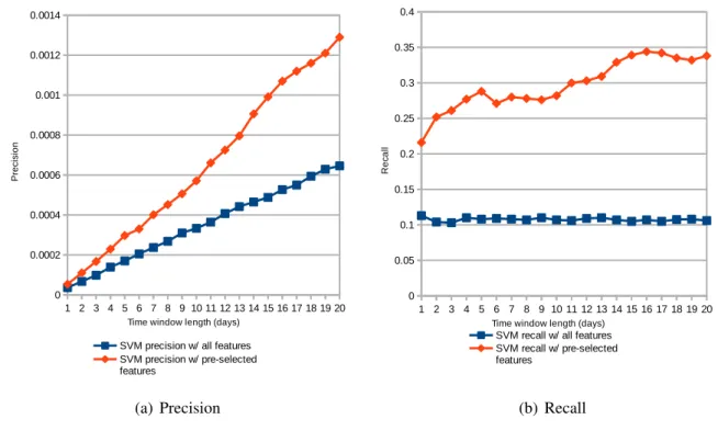
3.1 Precision and Recall of SVM for varying time window length with and without feature selection . . . 36

3.2 Precision and Recall of RF for varying time window length with and without feature selection . . . 37

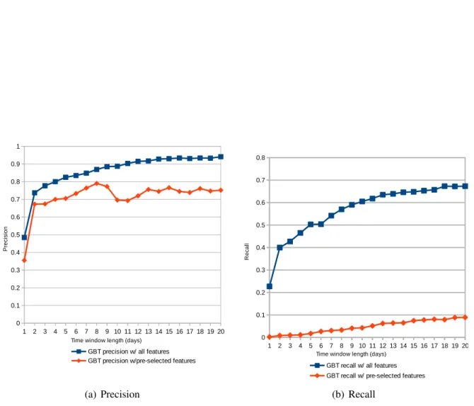
3.3 Precision and Recall of GBT for varying time window length with and without feature selection . . . 38

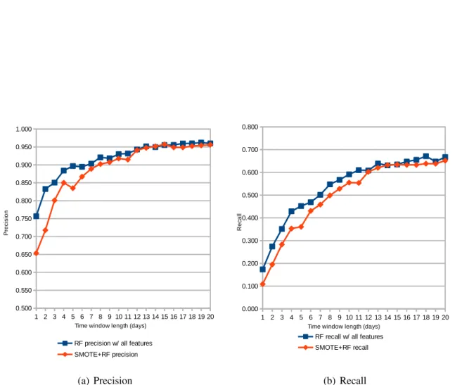
3.4 Precision and Recall of the RF model for varying time window length with and without feature selection . . . 39

5.1 Illustration of Federated Active Learning . . . 66

5.2 Performance with regards to number of hosts . . . 71

5.3 Performance with regards to the number of communication rounds . . . 72

5.4 Performance with regards to the request budget . . . 73

(11)

(12)

List of Tables

1.1 Summary of maintenance paradigms . . . 5

2.1 Summary of related work in predictive maintenance . . . 13

2.2 Summary of related work in applied machine learning . . . 22

3.1 Description of SMART parameters . . . 32

3.2 Execution time of the methods . . . 37

4.1 Illustration of an aeronautical system text log . . . 44

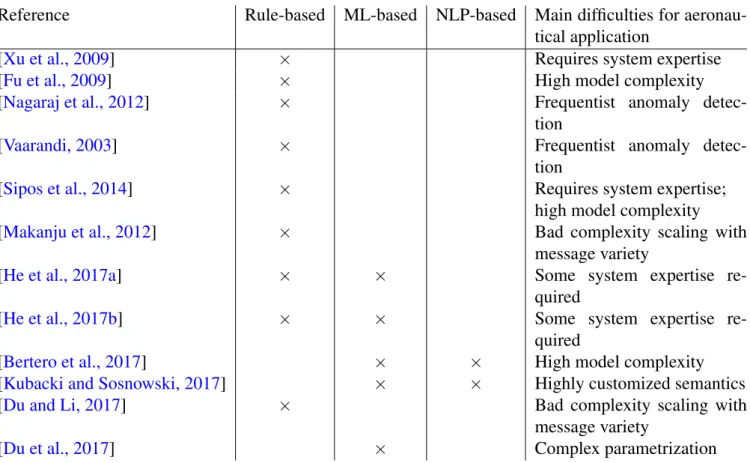
4.2 Summary of related work in log parsing and log mining . . . 48

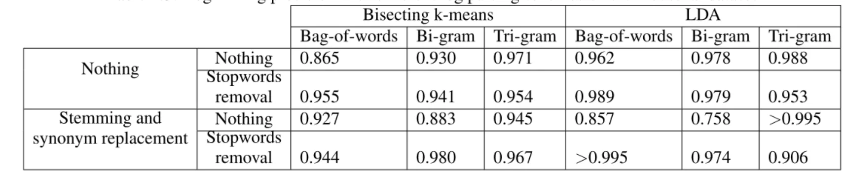
4.3 Log mining precision with different log parsing schemes on the industrial dataset 54 4.4 Log mining recall with different log parsing schemes on the industrial dataset . 55 4.5 Log mining F-score with different log parsing schemes on the industrial dataset 56 4.6 Performance comparison against state-of-the-art approaches on the HDFS bench-mark dataset . . . 57

4.7 Example of raw HDFS text log . . . 58

(13)

(14)

(15)

Acronym Description

ADMM Alternating Direction Method of Multipliers CNN Convolutional Neural Network

DNN Deep Neural Network DT Decision Tree

EASA European Union Aviation Safety Agency FAA Federal Aviation Agency

GBT Gradient Boosted Tree GD Gradient Descent

GPU Graphical Processing Unit HDD Hard Drive Disk

HDFS Hadoop File System IoT Internet of Things

IPLoM Iterative Partitioning Log Mining IID Independent and Identically Distributed

L-BFGS Limited memory Broyden-Fletcher-Goldfarb-Shanno LCS Longest Common Subsequence

LDA Latent Dirichlet Allocation LR Logistic Regression

LSTM Long Short-Term Memory MIL Multiple Instance Learning ML Machine Learning

MTBF Mean Time Before Failure NLP Natural Language Processing PCA Principal Component Analysis RBM Restricted Boltzmann Machine ReLU Rectiﬁed Linear Unit

RF Random Forest

SGD Stochastic Gradient Descent

SMOTE Synthetic Minority Oversampling TEchnique SVM Support Vector Machine

(16)

Chapter 1 Introduction

Section1.1details the general context of the thesis and the problematic it is meant to address. The next section1.2 starts with a characterization of aeronautical systems with a focus on the speciﬁcities that justify the need to study them separately from other industrial systems. Then, an explanation of the concept of predictive maintenance for industrial systems and the reason why Machine Learning is considered particularly promising to achieve it are given.

Finally, by cross-examining the problematic of the thesis, the speciﬁcities of aeronautical systems and the contributions of Machine Learning, the essential steps of the thesis are identi-ﬁed and the contribution roadmap formalised in section1.3.

1.1 General context and problem statement

The goal of this thesis is to propose a real-time predictive maintenance system adapted to the specific challenges of aeronautical systems. The corporation Safran, of which my hosting com-pany TriaGnoSys is a subsidiary, is an aeronautical equipment supplier and , in this capacity, has many integrated sensors deployed in a variety of aircraft. The measurements made by the sensors during the flight are collected and stored after the flight. Currently, they are usually

(17)

analysed by an operator if and only if an anomaly is detected.

In order to improve the reliability of our equipments and to reduce maintenance costs, it would be preferable to make use of those measurements to predict anomalies before they happen. Sev-eral aeronautical constructors such as Airbus and Boeing have already adopted this approach by using Machine Learning in order to deal with the vast amounts of data but in a strictly ofﬂine manner, that is to say that they make use of their data only after landing. Some speciﬁcities of aeronautical systems, detailed in the next section, already need to be addressed at this stage. This application is not trivial and though predictive maintenance models for aeronautical sys-tems already exist, the detail of their implementation is not publicly available.

To extend this work further, the goal of this thesis is to set a predictive maintenance model for aeronautical systems that can operate during the flight. This would increase the security and reliability of aeronautical systems and improve the organization of the maintenance operations after landing. The main difference imposed by this goal concerns the computation resources. Offline models can use as many computation servers as necessary in the very favourable context of a data center whereas a model used in flight must use the on-board resources and follow a number of constraints to be allowed on board. Those constraints are imposed by aeronautical certification agencies and include, among others, fault tolerance, high reliability and isolation with regards to other on-board software in case of malfunction.

The solution to those limitations that is investigated in this thesis is the use of a data link be-tween the aircraft and the ground. Indeed, it is becoming the norm for commercial ﬂights to offer connectivity with the Internet and it is one of the services in which the hosting company is specialised in. This connectivity can be achieved in different ways with different kind of satellite connections or through direct air-to-ground communication. Figure1.1presents a sim-pliﬁed representation of the systems involved.

The issue that remains is that, no matter what connectivity solution is used, compared to ground connections, the data link between the aircraft and the ground is always ﬁnancially more ex-pensive, has a very limited bandwidth and a limited availability. Therefore, transmitting all the measurements made by the on-board sensors to the ground following a cloud computing paradigm is not realistic. As such, some computations have to take place on-board to transmit only relevant data. The core of this thesis is to determine an ensemble of two learning models, one on board and the other on the ground that can collaborate on the anomaly prediction prob-lem and a software architecture able to support them in order to produce accurate estimates of anomaly risks on board without saturating the data link.

(18)

(19)

more important a system is to the safety of the aircraft, the higher the requirements will be. The exact steps needed to certify an aeronautical system will therefore vary slightly from one system to another and are outside the scope of this thesis however there are enough similarities in the certiﬁcation process to lead to similarities in the aeronautical systems and that is of interest for this work.

• The ﬁrst and most obvious requirement, characteristic of aeronautical systems, is their high reliability. Reliability in this case is deﬁned as 1 − probability of failure over a

period of time. Mean Time Before Failure (MTBF) is often used as a way to express the

expected lifetime of an aeronautical system based on its reliability.

• A second specificity of aeronautical systems induced by the certification process is the need to closely monitor their performances of aeronautical system and ensure the conser-vation of the data obtained through this monitoring. This is required in order to demon-strate that the aeronautical system meets the certification specifications.

• A third specificity of aeronautical systems is the difficulty to change them. The certifi-cation process is costly, both financially and in terms of time, and introducing changes to a system during the process creates additional costs. Similarly, an update to a previ-ously qualified system also has to go through a certification process, though simpler than the process for a new system. Because of this, there is a considerable delay between the design of an aeronautical system and its actual implementation in the field.

• Lastly, though desirable, the goal of perfect isolation of aeronautical systems from each other is, by design, impossible to achieve as they are co-located with every other on-board system and have to share resources such as power supply. Aeronautical systems are always interdependent at some level.

1.2.2 Predictive maintenance

As explained in the problem statement, the goal of this thesis is to achieve a better predictive maintenance for aeronautical systems. Predictive maintenance is a popular topic for industrial applications as a way to increase reliability and reduce costs and waste. Its principle is to monitor the condition of the system to maintain in order to repair or replace it just in time before it fails. There are two other approaches to maintenance.

The ﬁrst one, corrective maintenance, replaces a system after it has started malfunctioning. It has the advantage of minimizing the number of required maintenance operations but does not allow for the planning of those operations and, in the case of interdependent systems, for example in an assembly line, the consequences of a dysfunction can have an impact beyond the system to maintain that might not be acceptable, like a complete halt of production in the case of the assembly line.

(20)

1.2. Definition of general and industrial concepts

The second approach, called preventative maintenance, replaces and repairs systems in a scheduled manner based on statistics of their reliability. This approach is favoured for criti-cal systems where the consequences of a failure are considered unacceptable such as medicriti-cal systems or for systems where the cost of a planned maintenance is signiﬁcantly lower than an unplanned one. For the example of an assembly line, making a planned maintenance when the line is not being operated for example. The preventative approach however leads to the repair and replacement of systems that are still in working condition which implies that too many maintenance operations are taking place and that there is a waste of spare parts. It is also possi-ble that failures happen before the scheduled maintenance as the condition of the system is not actively monitored so the number of unplanned maintenance operations is reduced but is not zero.

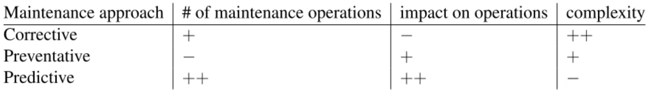
In contrast, the predictive maintenance approach aims at replacing parts only when it is ne-cessary like in the corrective approach but without letting the system fail like in the preventative approach by modelling its behaviour based on monitoring data. When perfect accuracy is not possible, it is also often possible depending on the model used to balance the sensitivity of the prediction with regards to the relative cost of planned versus unplanned maintenance. It has the downside of requiring the implementation of sensors to monitor the equipment. The table1.1

summarizes the strengths and drawbacks of the three maintenance approaches identiﬁed. Maintenance approach # of maintenance operations impact on operations complexity

Corrective + − ++

Preventative − + +

Predictive ++ ++ −

Table 1.1: Summary of maintenance paradigms

Predictive maintenance is therefore very desirable and, in theory, superior to the other ap-proaches when sensors are easily implementable. It is also however technically more complex as it relies on a failure prediction model that is potentially difﬁcult to obtain whereas corrective maintenance only requires to detect the malfunction and preventative relies on the system life expectancy. The failure prediction model can be obtained from a formal analysis of the system by a domain expert in the order to determine what can be deduced about the state of the system from the monitored parameters. However, when studying the interactions of multiple inter-dependent systems, the complexity of a formal analysis quickly becomes intractable with the number of potential cross-system interactions. Such an approach can still be undertook at con-siderable costs for extremely critical applications to ensure, for example, the safety of nuclear power plant installations but such endeavours are not possible for every industrial system.

Even though formal analysis are not always possible, there is another approach that consists in studying statistical correlations between the system failure events and the monitored param-eters. Until recently, this approach required considerable computation resources to achieve

(21)

acceptable levels of accuracy on complex systems. With the latest advances in Machine Learn-ing applications, it is however becomLearn-ing increasLearn-ingly simple to sift through amounts of data that would have been considered intractable a decade earlier.

1.3 Presentation of the thesis

In the two previous sections, we have identified the goal of the thesis, the specificities of the aeronautical application field and the most suitable approach to create the failure prediction model. Based on this, we identify the problems that this thesis needs to address in order to reach a conclusion and structure it around these problems.

A natural ﬁrst step as a preamble to this work is to present the background that it is necessary to follow the contributions presented therein. As such, chapter2contains a synthetic overview of the state of the art of the domain.

Then, the first problem that we identify is tied to the fact that aeronautical systems are reliable. While obviously being a desirable trait for any industrial system, it also carries the implication that there are few examples of failure to observe. That is a problem from a Machine Learning perspective because for the statistical model to be accurate, it requires as many exam-ples of failures as possible. If the failures are too rare, it will be difficult to generalize correctly the model from the observations. A simple example and a common situation for aeronautical systems such as engines or navigation sensors would be a critical system that only had a single failure in several years of operation. Because of the criticality of the system, a failure predic-tion model as accurate as possible is desired but since there is only a single known example of failure it is not possibly to obtain a statistically conclusive result. A second aspect of this problem is the balance aspect. Many Machine Learning classification algorithms are designed to learn from a balanced dataset, that is to say a dataset where the classes to discriminate are in equal proportions. For aeronautical systems, because of the scarcity of failures, this ratio can typically be in the range of 1:100, 000. A first step in the thesis is therefore to understand the extent of this problem and study which methods or combination of methods from Machine Learning can operate on aeronautical systems in this situation of rare events prediction. We do so in chapter3. The results of this contribution have been published in the proceedings of the 16th _{IEEE International Conference on Machine Learning and Applications (ICMLA 2017) as}

"Predictive models of hard drive failures based on operational data" by Aussel, N., Jaulin, S., Gandon, G., Petetin, Y., Fazli, E. and Chabridon, S. [Aussel et al., 2017].

The second problem that we need to acknowledge is that because of the costs, ﬁnancial and in terms of time, associated with updating aeronautical systems it is not reasonable to make changes necessary for them in order to enable the work of this thesis. To put it in another way, we cannot decide which parameters to monitor for the failure prediction model. We have to use the parameters that are already monitored. Otherwise the delay in the update process and the time needed to gather a sufﬁciently large sample that contain multiple failures would widely

(22)

1.3. Presentation of the thesis

exceed the duration of the thesis. Nevertheless a positive aspect is that aeronautical systems are already closely monitored so there is already data to work with but the data collection process cannot be changed. A second important step in the thesis is therefore to study how to adapt Machine Learning method to the pre-existing data format. We conduct this study and propose our own approach in chapter4. The results of this contribution have been published in the pro-ceedings of the 26th _{IEEE International Symposium on Modeling, Analysis, and Simulation of}

Computer and Telecommunication Systems (MASCOTS 2018) as "Improving Performances of Log Mining for Anomaly Prediction Through NLP-Based Log Parsing" by Aussel, N., Petetin, Y. and Chabridon, S. [Aussel et al., 2018].

Finally the last problem to address in the thesis is the distributed learning between the air-craft and the ground station. Here the contribution is a new algorithm that can be run in parallel on one host with real-time data sources and limited computational power, the aircraft, and an-other host with high computational power but no access to recent data, the ground station. The requirements of the algorithm are to be able to run with a limited communication budget and to offer guarantees on the accuracy of its decision on the aircraft side. This is done in chapter5.

(23)

(24)

Chapter 2 Fundamentals and State of the Art

2.1 Introduction

In this chapter, we present a synthetic review of related work. This review is organised by themes in three sections. The ﬁrst one focuses on the current state-of-the-art in terms of pre-dictive maintenance distinguishing frameworks and methods applicable in a generic industrial context and in an aeronautical context. We will rely on it to determine what are the best practices and useful metrics used in this ﬁeld to measure our results.

Then an overview of Machine Learning fundamentals is given. Machine Learning is used in this thesis to determine the statistical model that enables anomaly detection so we provide a deﬁnition of Machine Learning and we detail the standard methods used to build a Machine Learning pipeline step-by-step from data pre-processing to post-processing.

Finally, we review the current state-of-the-art in the matter of Distributed Learning. This is necessary to set the context of the solution to propose to the thesis problem statement.

2.2 Predictive maintenance of industrial systems

2.2.1 General case

Predictive maintenance is about monitoring the state of a system to trigger maintenance just in time in order to maximize maintenance efficiency. A good introduction to the field of predictive maintenance can be found in [Mobley, 2002] with an explanation of predictive maintenance the-ory, its financial and organisational aspects, concrete examples focused on industrial machinery and guidelines on how to set up and sustain a predictive maintenance program.

There are plenty of studies about predictive maintenance focusing on its organisational or lo-gistics aspects such as [Shaﬁee, 2015]. They are essential to ensure that the changes induced on the maintenance policy actually translates into a net measurable improvement for the operator of the system or, to put it in another way, how the failure predicted by the model can be trans-lated into a concrete business process and how the efﬁciency of this process can be measured. For this, aspects like cost of unplanned versus planned maintenance need to be considered as well as location and availability of spare parts and maintenance personnel and associated costs. A notable study, [Horenbeek and Pintelon, 2013], focuses on the interaction of monitored com-ponents and how optimizing the cost of the maintenance policy of the whole system is not as simple as optimizing the maintenance policy at component level. This study models a stochastic dependence between components to show that the degradation of a component and its failure has an impact on other components with possible cascading effects of primary failure of a com-ponent inducing secondary failures of other comcom-ponents. It also introduces a structural and economic dependence to model the fact that simultaneous maintenance of several components at once is cheaper than individual of each component one by one. Nevertheless, since the focus of this thesis is on the production of the failure prediction model, the organisational and logistics

(26)

2.2. Predictive maintenance of industrial systems

aspects are not explored further here and are left for future work.

There is also plenty of work focusing on the technical implementation of predictive main-tenance, that is to say how to get from the observations from the sensors monitoring the system to the failure prediction model. Multiple approaches to this problem exist. In [Hashemian, 2011], the authors propose a review of the state-of-the-art techniques available in 2011 with a particular focus on industrial plants, the type of sensors that are available for various systems and the effect on the observations for various types of anomaly. In general there are two dif-ferent ways to establish a failure prediction model based on observations. The so called model based approach starts from a theoretical physical model of the system to determine what would observations indicative of an imminent failure look like or the statistical approach which starts from a history of observations to try to infer a failure prediction model.

A good example of predictive maintenance based on a physical model can be found in [ Maz-zoletti et al., 2017]. This study leverages expert knowledge about the system it examines, here a permanent magnet synchronous machine, to build an analytical theory of how a malfunction may impact sensor measurements and then validates experimentally the theory. This approach has been historically adopted in many other predictive maintenance studies such as [Bansal et al., 2004] or [Byington et al., 2002]. However the more complex the system the more difﬁ-cult it is to apply this approach. In the case of interdependent systems, which, as we have seen, aeronautical systems generally are, building an exhaustive analytical theory would require ex-perts for every system involved as well as exex-perts in the interaction of those systems making it impossible to scale this approach to, for example, an entire aircraft.

The other approach to failure prediction for predictive maintenance that has been gaining in popularity lately is the statistical approach found for example in [Li et al., 2014a] and [Ullah et al., 2017]. The goal of this approach is to ﬁnd correlations between sensor measurements and system failures and build the failure prediction model based on those without necessarily resorting to the physical interpretation of the measurements. A very simple illustration would be the following: let us assume that our system is equipped with a sensor SA measuring the

parameter A and let us assume that we found that when A < 5 the daily failure rate of our sys-tem is 1% and when A > 5 the daily failure rate is 99%. Without knowing what A represents or what unit it is expressed in, we can already intuitively propose a simple threshold rule for failure prediction, when A > 5 predict failure and else predict non-failure. Of course, situa-tions are rarely so clear cut and, even so, the next question to answer would be can we predict when the threshold will be exceeded so there is an abundance of work on how to generate the failure prediction model from the observations. In [Grall et al., 2002], a speciﬁc category of system is studied, deteriorating systems, monitored by a sensor measurement characterized by a stochastic increasing process and a failure threshold. A method is then proposed to identify the parameters of the stochastic process from historical observations and to derive failure pre-diction rules from them. This approach is very interesting as it foregoes the need for expert knowledge of the system but as it still has analytical components there is still a difﬁculty in

(27)

scaling it up when the number of sensor measurements increases or when we cannot make as-sumptions a priori on their behaviour. The latest solution that has been found in that case is to use a Machine Learning approach to automate the extraction of relevant features and rules when there is a large volume of data available. [Li et al., 2014a] and [Ullah et al., 2017] provide two recent examples of complex models, a Decision Tree and a Multi-layer Perceptron, learned through Machine Learning techniques. We explain the principle of those techniques in the next section2.3dedicated to Machine Learning fundamentals.

2.2.2 Aeronautical systems

The situation for machine learning techniques applied to aeronautics is quite complicated. There is ample documentation of products being sold by aircraft manufacturers such as Boeing An-alytX3 _{or Airbus Skywise}4 _{but few details about them are public. Datasets are obviously not}

publicly available and, even when a scientiﬁc publication exists, neither are the implemen-tation of the algorithms used. An illustration of this can be found in [Burnaev et al., 2014] and [Kemkemian et al., 2013].

It is also possible to ﬁnd additional references in patents held by manufacturers but the level of detail available is lower yet. The following patents [Song et al., 2012] and [Kipersztok et al., 2015] illustrate that fact. It is also worth noting that the volume alone of patents held by the aircraft manufacturers, more than 54.000 for Boeing alone as of 2019, makes it impossible to conduct an exhaustive review.

For these reasons, despite the existing concrete applications of machine learning for pre-dictive maintenance of aeronautical systems, it is still necessary to carefully study them in this thesis.

A notable exception is the thesis recently made public [Korvesis, 2017]. Taking the slightly different point of view of an aircraft manufacturer, it focuses on the issue of automation of Ma-chine Learning for predictive maintenance processes while this thesis considers the problem of software architecture and distributed execution. It is nevertheless worth noting that similar ob-servations regarding the applicability of Machine Learning techniques to aeronautical systems with regards to rare event predictions were reached concurrently in this thesis and in [Korvesis, 2017].

In the table 2.1, we summarize the contributions of the articles we discuss here for this thesis.

3_{https://www.boeing.com/company/key-orgs/analytx/index.page} 4_{https://www.airbus.com/aircraft/support-services/skywise.html}

(28)

2.3. Machine Learning fundamentals

Reference Comment

[Mobley, 2002] General introduction

[Shaﬁee, 2015] Logistics and process aspects [Horenbeek and Pintelon, 2013] Multi-component complexity

[Hashemian, 2011] State-of-the-art for industrial plants; focus on sensors [Mazzoletti et al., 2017] Predictive maintenance bqsed on physical models [Bansal et al., 2004] Predictive maintenance bqsed on physical models [Byington et al., 2002] Predictive maintenance bqsed on physical models [Li et al., 2014a] Statistical approach with Decision Tree

[Ullah et al., 2017] Statistical approach with Multi-layer Perceptron [Grall et al., 2002] Predictive maintenance for deteriorating system [Burnaev et al., 2014] Aeronautical application; dataset not released [Kemkemian et al., 2013] Aeronautical application; dataset not released

[Korvesis, 2017] Similar topic but focus on automation; datasets not released Table 2.1: Summary of related work in predictive maintenance

2.3 Machine Learning fundamentals

This section is meant to give an overview of Machine Learning terminology and the techniques that are discussed in this thesis. Machine Learning is a very active ﬁeld of research at the moment. For a more detailed introduction to the ﬁeld from a statistical perspective, we rec-ommend [Friedman et al., 2001]. To quote it, Machine Learning is about extracting knowledge from data in order to create models that can perform tasks effectively. Unpacking that statement, we can identify three points:

• Machine Learning is working from data. This means that the inputs are observations, measurements, recordings with no assumption at this stage on their format. They can be numerical or categorical, continuous or discrete, text ﬁles or video recordings. The only thing that is certain is that we do not have access to a model to generate this data and have to progress empirically towards it. This variety of inputs partially explains the variety of learning methods that have been developed. A ﬁrst difference that is usually made at this stage is whether the data is labelled or not which, in this context, means that for a given observation, we know the desired output. When the desired output is known, the data is labelled and the learning is called supervised. When the desired output is not known, the learning is called unsupervised. A hybrid situation where some of the data is labelled and some is not is possible in which case the learning is called semi-supervised.

• The expected output is a model that performs a task. Once again, this formulation is very generic and carries no assumption on the nature of the task. A generic denomination is

(29)

often made depending on whether a categorical or a numerical output is expected. In the ﬁrst case, the model is called a classiﬁcation model and in the second it is called a regression model.

• There is an expectation of efﬁciency for the model. The question of performance metrics is essential for a Machine Learning approach as it is necessary to guide the learning process. A function called the loss function is used to determine how well the current model ﬁts the data.

The categories defined here are very broad and do not necessarily describes every method available. For example, reinforcement learning is a popular sub-field of Machine Learning interested in learning action policies using algorithms such as Q-learning [Watkins and Dayan, 1992] which is traditionally considered to be neither a classification nor a regression model. Nevertheless these categories are part of the standard terminology in Machine Learning and are a useful way to quickly describe the application range of a learning method.

Regarding the notations that we will use, roughly speaking, we have at our disposal a set of multidimensional observations x ∈ Rd_{, (x}

1, x2, ..., xd). For example, x can represent the

data or a transformation of the data acquired by the sensors. For a given x, we associate a label

y ∈ R for a regression problem or {0, 1} for a binary classiﬁcation problem with 0 coding for

no event and 1 for event. The objective consists in predicting the label y associated to a data x.

2.3.1 Logistic Regression

Logistic Regression (LR) [Friedman et al., 2001] is a method widely used for regression and classiﬁcation where predictions rely on the following logistic function:

φ(x) = 1

1 + exp−w0−P d i=1wixi

(2.1) In the regression case, φ(x) is interpreted as the estimate for y. In the classiﬁcation case, φ(x) is interpreted as the probability that y = 1 given x. Consequently, the objective is to estimate Pr(y = 1|x) and so (w0, · · · , wd) from {(x1, y1), · · · , (xN, yN)}.

LR can be trained several methods such as Stochastic Gradient Descent or Limited mem-ory Broyden-Fletcher-Goldfarb-Shanno algorithm (L-BFGS) [Bottou, 2010] depending on the computing resources available. A known limitation of the LR model is that it works poorly with time series, where the assumption that the observations {(x1_{, y}1_{), · · · , (x}N_{, y}N_{)} are}

indepen-dent is challenged.

2.3.2 Support Vector Machine

Support Vector Machine (SVM) is a technique that relies on ﬁnding the hyperplane that splits the two classes to predict while maximizing the distance with the closest data points [Cortes

(30)

2.3. Machine Learning fundamentals

and Vapnik, 1995]. With N the number of samples, xi the features of a sample, y its label and ~

w the normal vector to the hyperplane considered, b the hyperplane offset and λ he soft-margin,

the SVM equation to minimize is:

f ( ~w, b) = λk ~wk2₊ 1 N N X i=1 max(0, 1 − yi(w.xi− b)) (2.2)

It is worth noting that even if it was initially designed with separable data in mind, the equation remains valid even when some points are on the wrong side of the decision boundary [Cortes and Vapnik, 1995, Friedman et al., 2001] which means SVM is applicable even without the assumption that the data is separable. SVM can also be trained online using, for example, active learning techniques [Bordes et al., 2005].

2.3.3 Deep Neural Networks

Fully connected Deep Neural Networks (DNN) are popular architectures which aim at approx-imating a complex unknown function f(x), where x ∈ Rn_{is an observation, by f}

θ(x) [

Rosen-blatt, 1957] [Negnevitsky, 2001]. θ consists of the parameters of the DNN, the bias vectors

b(i) and the weight matrices W(i) for all i, 1 ≤ i ≤ P , and f_θ_{(x) is a sequential}

composi-tion of linear funccomposi-tions built from the bias and from the weights, and of a non-linear activacomposi-tion function g(.) (eg. the sigmoid g(z) = 1/(1 + exp(−z)) or the rectiﬁed linear unit (ReLu)

g(z) = max(0, z)) [Cybenko, 1989][LeCun et al., 2015].

Parameters θ = {b(i)_{, W}(i)_{} are estimated from the back-propagation algorithm via a}

gra-dient descent method based on the minimization of a cost function Lθ((x1, y1), · · · , (xN, yN))

deduced from a training dataset [Rumelhart et al., 1988].

However, when the objective is to classify high dimensional data such as colour images with a large number of pixels, fully connected DNN are no longer adapted from a computational point of view.

2.3.4 Convolutional neural networks

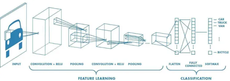
Convolutional Neural Networks (CNN) aim at dealing with the previous issue by taking into account the spatial dependencies of the data [Albawi et al., 2017]. More precisely, data are now represented by a 3-D matrix where the two ﬁrst dimensions represent the height and the width of the image while the depth represents the three colour channels (R,G,B).

Next, as fully connected DNN, CNN consists in building a function ftheta(x), where x ∈ Rd1

× Rd2

× Rd3, by the sequential composition of the following elementary steps :

• a convolution step via the application of convolution ﬁlters on the current image. Each ﬁlter is described by a matrix with appropriate dimensions;

(31)

Figure 2.1: Example of a CNN architecture • the application of an activation function g(.) such as the ReLu; • a pooling step to reduce the dimension of the resulting image.

After the recursive application of these three steps, the output image is transformed into a vector of Rn_{and is classiﬁed via a fully DNN described in the previous paragraph [}_{Krizhevsky et al.,}

2012]. A general CNN architecture is displayed in Fig.2.3.4.

Again, the back-propagation algorithm estimates the parameters (weights and bias of the ﬁnal DNN and of the convolution matrices) of the CNN.

2.3.5 Decision Tree

Decision Tree (DT) [Breiman, 2017] is a supervised learning method that can be used for both classiﬁcation and regression. Its goal is to recusively create simple decision rules to infer the value of the target. To do so, it determine each split as follow: given m the current node to split,

Qmthe data available at that node, Nmthe number of samples in Qm, θ the candidate split, nlef t

and nright the amount of sample split respectively to the left and right of the node and H the

impurity function, nlef t Nm H(Qlef t(θ)) + nright Nm H(Qright(θ)) (2.3)

This step is repeated until Nm = 1, i.e. the split is pure, composed of a single class, or the

(32)

2.4. Applied Machine Learning

2.3.6 Random Forest

Random Forest (RF) improves on DT by combining several decision trees each trained on boot-strapped samples with different attributes. A process called bagging is used. Its principle is that to train N trees, for each tree, a subset of the features and a subset of the observations are sampled with replacement. New predictions are then made based on a vote among the different decision trees [Criminisi et al., 2012].

2.3.7 Gradient Boosted Tree

Finally, Gradient Boosted Tree (GBT) is another ensemble technique based on decision trees. Instead of training random trees like in RF, the training takes place in an iterative fashion with the goal of trying to minimize a loss function using a gradient descent method [ Crim-inisi et al., 2012]. Example of log loss function characterized by the formula: 2 ×PN

i=1log(1 +

exp(−2yiF (xi))) where N is the number of samples, xiand yirespectively the features and the

label of the sample i and F (xi) the predicted label for sample i. This function is minimized

through 10 steps of gradient descent.

2.4 Applied Machine Learning

In this section we take a more specific interest into three sub-fields of Machine Learning that make use of the techniques described in section2.3to tackle specific challenges that are of use to this thesis.

2.4.1 Distributed Learning

Many Machine Learning techniques such as DNNs are notorious for requiring large amount of data to train effectively [Krizhevsky et al., 2012]. As a result, it is not unusual when employing these techniques to have to consider the question of computational resource usage. An obvious solution to reduce this usage would be to simply invest in a more powerful processing unit but this solution is not always practical. Another way that can be investigated is to share the computation load across multiple cores or multiple processing units.

The use of multiple cores to take advantage of the embarrassingly parallel nature of the computations in DNNs, largely credited for the rise of deep learning methods in popularity, can be found in the implementation of Machine Learning on Graphical Processing Units (GPUs). It is sometimes called Parallel Learning and an example of a study on this can be found in [ Sierra-Canto et al., 2010]. We will not investigate this further as we are more speciﬁcally interested in learning that happens between processing units in different hosts. The approach of using sharing the computation load across multiple processing units is called distributed learning. It

(33)

can take different shapes depending on how the processing units are allowed to communicate with each other. [Peteiro-Barral and Guijarro-Berdiñas, 2013] is a survey of some of the work done on this topic as of 2013.

Regarding the different characteristics of processing unit communications to take into ac-count that are important to correctly frame the problem, several borrows from the ﬁeld of dis-tributed systems. We can mention:

• Centralized and decentralized learning: this question, very common in distributed sys-tems, is about the roles of the hosts and whether one of them has a privileged role of coordinator or master. A well-known example of a centralized learning method is the parameter server for centralized asynchronous Stochastic Gradient Descent (SGD) de-scribed in [Li et al., 2014c] for example. In this approach, a central server called the parameter server distributes data and workload asynchronously to a group of workers while maintaining a set of global parameters. After receiving updates from the work-ers, the parameter server aggregate them and update the global model. An example of work in centralized learning on an algorithm other than SGD can be found in [Zhang and Kwok, 2014] where the method of Alternating Direction Method of Multipliers (ADMM) is used to ﬁnd a distributed consensus asynchronously by using partial barriers. In con-trast, in decentralized learning, every host has the same role. In [Watcharapichat et al., 2016], a variant of GD for Deep Learning is presented with the explicit goal of getting rid of the parameter servers in order to remove potential performance bottlenecks. This variant relies on exchanging partitions of the full gradient update called partial gradi-ent exchanges. Another example of decgradi-entralized learning can be found in [Alpcan and Bauckhage, 2009] where the authors propose a decentralized learning method for SVM by decomposing the SVM classiﬁcation problem into relaxed sub-problems.

• Data and model parallelism: as a ﬂip side to distributed system bit-level parallelism and task-level parallelism, the expression data parallelism and model parallelism are used. They do, however, cover very similar concepts. Data parallelism expresses the idea that the tasks between the hosts are shared by distributing the dataset between them while for model parallelism operations are executed in parallel by the hosts on the same dataset. They are illustrated in ﬁgure 2.4.1. A notable difference between model parallelism in distributed learning and task parallelism in distributed systems is that model parallelism does not necessarily imply that the operations are done on the same data. It is also worth noting that data and model parallelisms are not mutually exclusive. In [Li et al., 2014c], for example, the parameter server distributes both the data and the tasks between the workers. This makes sense because fragments of a given dataset are assumed to represent the same distribution and hence the results can be combined in the same model.

• Synchronous and asynchronous: the distinction between synchronous and asynchronous communication in distributed learning is completely analogous to the one in distributed

(34)

(35)

class imbalance (though with a much less drastic ratio). The most signiﬁcant difference with the prediction in aeronautical systems, beside the order of magnitude change in class imbalance ratio, is that it is a decentralized algorithm with communication between hosts which is not a realistic hypothesis for aircraft. Another problem that it does not address is the fact that the performance of individual models is not controlled meaning that it is not lower bounded and that there are no mechanisms to correct a potential drift of a local model. It makes sense in the situation considered in [Valerio et al., 2017] but it is a requirement that needs to be addressed in the aeronautical use case.

2.4.2 Active Learning

Another field of Machine Learning that we want to detail is Active Learning. Active Learning is a field of semi-supervised learning where a third-party called an oracle can provide missing labels on request. It is traditionally not considered a sub-field of Distributed Learning and is applied in a very different context where data labelling requires the intervention of a human operator that is both costly and slow and the goal is to provide a strategy to get the best model accuracy under a fixed request budget. A summary of the principles of Active Learning from a statistical perspective can be found in [Cohn et al., 1996]. From a practical perspective, active learning has historically been used with success for use cases such as spam filtering [Georgala et al., 2014], image classification [Joshi et al., 2009] or network intrusion detection [Li and Guo, 2007]. Different approaches are available for Active Learning and a survey summarizing them can be found in [Settles, 2009]. The most common approach for concrete applications is called pool-based active learning and described in [Lewis and Gale, 1994]. The assumption in this approach is that there is a large pool of unlabelled data and a smaller pool of labelled data available. The labelled data is used to bootstrap a tentative model and a metrics to measure the amount of information gain one can expect from a sample is defined. Some examples of metrics can be a distance metrics between the sample and the decision boundary of the model, the density of labelled data in the vicinity of the sample or the difference in the learned model with regards to the possible labels. Once the metrics is defined, the unlabelled samples that are expected to maximize the information gain are queried from the oracle then the tentative model is updated and the process is repeated until the expected information gain falls below a pre-defined threshold, meaning that no new label is expected to significantly change the model, or the query budget is spent.

A recent example of active learning can be found in [Gal et al., 2017] where a pool based approach is used on a dataset of skin lesion images with the goal to classify the images be-tween benign or malign lesions (melanoma). The unlabelled images that are selected by the active learning approach using the metrics BALD ([Houlsby et al., 2011]) are queried. In this benchmark, the labels are known so they are simply disclosed but in a real world application a dermatologist could be consulted.

(36)

2.4. Applied Machine Learning

Another example of active learning relevant to this thesis can be found in [Miller et al., 2014]. In the context of malware detection, the authors introduce the concept of adversarial active learning. In this situation, the oracle is a human annotator that can be either a security expert that is assumed to always provide the correct labels, a crowd-sourced non-expert that is less expensive from a query perspective but that can make mistakes which are modelled as noisy labels or an adversarial agent masquerading as a crowd-sourced non-expert that provides the wrong labels. While an adversarial hypothesis is not directly applicable to our context, the notion of having different oracles available that have different levels of reliability is relevant.

Finally, another approach to active learning in decision trees can be found in [De Rosa and Cesa-Bianchi, 2017]. Here the approach is not pool-based but stream-based, that is to say that the algorithm is receiving a stream of unlabelled samples and does not have access to the complete pool which proscribes the greedy approach of evaluating every sample for information gain and selecting the best. In this article, a decision tree is trained and when a new sample is classified through it the confidence that is evaluated is not the confidence in the classification of the sample but in the optimality of the model. To put it differently, when a new leaf is added to the tree, the comparison is made between the ideal decision tree that could have been made if the true distribution of the samples were known and the expected performance of the current tree and, if the difference is found to exceed a certain threshold, labels are requested to minimize to risk of selecting a sub-optimal split for the new leaf. The points that are the most relevant for this thesis is that, by moving away from a greedy approach, we can ensure that the computation cost remains manageable, making this algorithm suitable for an on-board implementation and the notion of approaching the uncertainty in terms of bounded risks for the model to be sub-optimal instead of considering sample misclassification makes it possible to directly manage the trade-off between the communication budget and the quality of the model.

2.4.3 Federated Learning

A last sub-field of Distributed Learning that we would like to detail here is called Federated Learning. This term was coined rather recently in [McMahan et al., 2016]. The first use case described was the distributed learning of a centralized model for image classification and lan-guage modelling on mobile devices. In this situation, several assumptions made on previous works in distributed learning are not satisfied anymore. In particular, in this context, there is a privacy concern with the data proscribing any transfer of raw data between the central server and the clients, the data is massively distributed between a very large number of clients whose availability may change suddenly and the data cannot be assumed Independent and Identically Distributed (IID) between clients. Each one of these issues has already been studied individually in Distributed Learning but they cumulatively make for a challenging problem. In [McMahan et al., 2016], a solution to learn a DNN in this context is proposed. It uses iterative averaging of synchronous SGD over a random subset of clients to update a central model that is then

(37)

forwarded to the queried clients at each iteration.

Several publications are focused on improving different aspects of this method. In [Koneˇcn`y et al., 2016], the communication efﬁciency is improved through several tricks like random masks, update quantization and structured updates. In [Bonawitz et al., 2016], the focus is put on establishing how to ensure that the data used by the client in an update cannot be deduced from the update itself from the server-side by using a client-side differential privacy approach with double masking. Conversely, [Geyer et al., 2017] also establishes how to mask whether a client participated at all in a differential update.

In general, the constraints characterizing the federated learning approach are also applicable to aircraft which are also numerous, with limited availability that can dynamically change and with data that is not IID from one aircraft to another.

It is worth noting however that Federated Learning has been developped so far with DNN applications in mind and, in particular, it is also compatible with SGD and not with DT based approaches that do not rely on SGD.

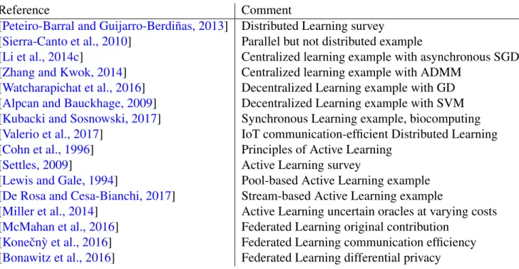
In the table 2.2, we summarize the contributions of the articles we discuss here for this thesis.

Reference Comment

[Peteiro-Barral and Guijarro-Berdiñas, 2013] Distributed Learning survey

[Sierra-Canto et al., 2010] Parallel but not distributed example

[Li et al., 2014c] Centralized learning example with asynchronous SGD [Zhang and Kwok, 2014] Centralized learning example with ADMM

[Watcharapichat et al., 2016] Decentralized Learning example with GD [Alpcan and Bauckhage, 2009] Decentralized Learning example with SVM [Kubacki and Sosnowski, 2017] Synchronous Learning example, biocomputing [Valerio et al., 2017] IoT communication-efﬁcient Distributed Learning [Cohn et al., 1996] Principles of Active Learning

[Settles, 2009] Active Learning survey

[Lewis and Gale, 1994] Pool-based Active Learning example [De Rosa and Cesa-Bianchi, 2017] Stream-based Active Learning example

[Miller et al., 2014] Active Learning uncertain oracles at varying costs [McMahan et al., 2016] Federated Learning original contribution

[Koneˇcn`y et al., 2016] Federated Learning communication efﬁciency [Bonawitz et al., 2016] Federated Learning differential privacy

(38)

2.5. Conclusion

2.5 Conclusion

In this chapter, we have presented several works related to the problem of this thesis focusing on Machine Learning fundamentals that will be useful for the next chapters and on state-of-the-art contributions to the problem at hand. The state-of-the-state-of-the-art contributions provide interesting clues to individually solve many of the problems we are faced with but none of the contributions offer a global solution that would ﬁt all the constraints of aeronautical systems. Starting from this observation, we can further reﬁne the questions that we address in the next chapters.

For rare event prediction in chapter 3, we have identiﬁed that most methods in applied Machine Learning are not particularly concerned with class imbalance but are compatible with multiple fundamental learning models and sampling methods. Therefore we will set out to compare the performance of these learning models and sampling methods in situations of class imbalance in order to determine which one would be the best choice to be at the core of the applied Machine Learning method.

For chapter4, dedicated to identifying the best way to adapt to the data format that is already available and that is very often for aeronautical systems free form text, we are also looking for pre-processing techniques that would not in theory depend on the applied framework. Thus, the approach will be similar in trying to ﬁnd the best methods without considerations such as distributed execution at this stage.

For chapter5, however, we have seen that existing methods, in particular in Federated Learn-ing and Active LearnLearn-ing, already provide multiple relevant solutions but not to every problem at the same time. Our approach will therefore be to ﬁgure out a new way to combine those existing solutions in the same applied Machine Learning framework.

(39)

(40)

Chapter 3 Rare Event Prediction for Operational

Data

3.1 Introduction . . . 26 3.1.1 General problem . . . 26 3.1.2 Hard Drives . . . 27 3.2 Related Work . . . 28 3.2.1 Previous studies . . . 28 3.2.2 Discussion . . . 29 3.3 Dataset . . . 30 3.3.1 SMART parameters . . . 30 3.3.2 Backblaze dataset . . . 31 3.4 Data processing . . . 31 3.4.1 Pre-processing . . . 31 3.4.2 Feature selection . . . 32 3.4.3 Sampling techniques . . . 33

3.4.4 Machine Learning algorithms . . . 34

3.5 Experimental results . . . 35

3.5.1 Post-processing . . . 35

(41)

In this chapter, we examine the applicability of different failure prediction techniques on operational data. To do so, we consider a public dataset of hard drive data to use as a proxy for conﬁdential aeronautical data. We try to apply existing methods to this problem, observe that their performances on operational data greatly differ from previous experiments and conclude on the relevant techniques for rare event prediction.

3.1 Introduction

3.1.1 General problem

One of the characteristics distinguishing aeronautical systems is the high importance that is given to their reliability as a way to ensure very high safety standards and minimize the cost of maintenance. As a result, failures of aeronautical systems are extremely rare. This makes the task of predicting them more difﬁcult for two reasons.

First, being rare events, it is more difficult to collect a dataset that includes a number of failures significant enough for statistical inference to be effective. In other words, if a given system fails on average once per year of operation and is deployed on a fleet of 20 aircraft, in order to collect a dataset containing at least 100 failures the data collection process should last on average 5 years. Such a duration is not reasonable in most cases. In order to work around that limitation, a practical solution is to work with artificially aged systems that are created by submitting systems in a controlled environment to stressful constraints that are believed to lead to precocious wear similar to that of older systems. For example, one could operate a system in the presence of high vibrations, temperature or with an unusual workload in order to artificially age it. However, this approach has been shown to introduce bias ([Pinheiro et al., 2007]) as the failures of artificially aged systems do not exactly match those of operational systems. When-ever it is possible, it is preferable to work with systems that are already extensively monitored for which a significant volume of data is already available. Those systems are, fortunately, not uncommon in aeronautics.

The second point making predictions difﬁcult in that situation is that the ratio between fail-ure samples, that is to say samples of a system that is about to fail, and healthy samples, from normally operating systems, is heavily skewed in favour of the latter. This is potentially prob-lematic for classiﬁcation because many learning techniques such as Logistic Regression or De-cision Tree operate best when the ratio between the two classes to predict is close to 1 ([Blagus and Lusa, 2010]). However, if we take the example of a system failing once per year on average again with a sampling rate, already pretty low, of 1 measure per hour we have on average about 8760 healthy sample for every failure sample for an imbalance ration in the range of 10−4_{. The}

two general ways to approach this difﬁculty is to either use sampling techniques to correct the imbalance by changing the sample population with the risk of introducing biases or by working

(42)

3.1. Introduction

with techniques that are more robust to imbalance.

Investigating these issues and more speciﬁcally the second point is necessary to design fail-ure detection for aeronautical systems but given the conﬁdential natfail-ure of industrial dataset and to ensure the reproducibility of the results, the investigation was conducted on a public dataset of another very reliable system, hard drive disks (HDDs).

3.1.2 Hard Drives

Hard drives are essential for data storage but they are one of the most frequently failing compo-nents in modern data centres [Schroeder and Gibson, 2007], with consequences ranging from temporary system unavailability to complete data loss. Many predictive models such as LR and SVM, analysed in section3.2, have already been proposed to mitigate hard drive failures but failure prediction in real-world operational conditions remains an open issue. One reason is that some failures might not be predictable in the ﬁrst place, resulting, for example, from improper handling happening occasionally even in an environment maintained by experts. However, this alone cannot explain why the high performances of the failure prediction models that appear in the literature have not mitigated the problem further. Therefore, the speciﬁcities of hard drives need to be better taken into account.

First of all, the high reliability of a hard drive implies that failures have to be considered as rare events which leads to two difficulties. The ideal application case of many learning methods is obtained when the classes to predict are in equal proportions. Next, it is difficult to obtain sufficient failure occurrences. Indeed, hard drive manufacturers themselves provide data on the failure characteristics of their disks but it has been shown to be inaccurate (see e.g. [Schroeder and Gibson, 2007], [Pinheiro et al., 2007]) and often based on extrapolating from the behaviour of a small population in an accelerated life test environment. For this reason, it is important to work with operational data collected over a large period of time to ensure that it contains enough samples of hard drive failures.

Another challenge is that the Self-Monitoring, Analysis and Reporting Technology (SMART) used to monitor hard drives is not completely standardized. Indeed, the measured set of at-tributes and the details of SMART implementation are different for every hard drive manu-facturer. From a machine learning point of view, there is no guarantee that a learning model trained to predict the failures of a speciﬁc hard drive model will be able to accurately predict the failures of another hard drive model. For this reason, in order to draw conclusions on hard drive failure prediction in general, it is important to ensure that the proposed predictive models are estimated from a variety of hard drive models from different manufacturers and also tested on a variety of hard drive models. Until now, this constraint was not taken into account prop-erly, probably because gathering a representative dataset has been a problem for many previous studies, impairing the generality of their conclusions. We rather focus on the Backblaze public

Real-time anomaly detection with in-flight data : streaming anomaly detection with heterogeneous communicating agents

HAL Id: tel-02191646

https://tel.archives-ouvertes.fr/tel-02191646

streaming anomaly detection with heterogeneous

communicating agents

Nicolas Aussel

To cite this version:

.

ü

'

0

'

0

O

)

O

)

n

-)

c

-TELECOM

Sud Paris

iJIWI

Real-time anomaly detection

with in-flight data:

streaming anomaly detection

with heterogeneous communicating

agents

Contents

Appendices

81

List of Figures

List of Tables

Chapter 1

Introduction

Contents

1.1

General context and problem statement

1.2.2

Predictive maintenance

1.3

Presentation of the thesis

Chapter 2

Fundamentals and State of the Art

Contents

2.1

Introduction

2.2

Predictive maintenance of industrial systems

2.2.1

General case

2.2.2

Aeronautical systems

2.3

Machine Learning fundamentals

2.3.1

Logistic Regression

2.3.2

Support Vector Machine

2.3.3

Deep Neural Networks

2.3.4

Convolutional neural networks

2.3.5

Decision Tree

2.3.6

Random Forest

2.3.7

Gradient Boosted Tree

2.4

Applied Machine Learning

2.4.1

Distributed Learning

2.4.2

Active Learning

2.4.3

Federated Learning

2.5

Conclusion

Chapter 3