Characterisation of time-varying underwater acoustic communication channel with application to channel capacity

HAL Id: hal-00473702

https://hal.archives-ouvertes.fr/hal-00473702

Submitted on 16 Apr 2010

HAL is a multi-disciplinary open access

archive for the deposit and dissemination of sci-entific research documents, whether they are pub-lished or not. The documents may come from teaching and research institutions in France or abroad, or from public or private research centers.

L’archive ouverte pluridisciplinaire HAL, est destinée au dépôt et à la diffusion de documents scientifiques de niveau recherche, publiés ou non, émanant des établissements d’enseignement et de recherche français ou étrangers, des laboratoires publics ou privés.

Characterisation of time-varying underwater acoustic

communication channel with application to channel

capacity

François-Xavier Socheleau, Jean-Michel Passerieux, Christophe Laot

To cite this version:

François-Xavier Socheleau, Jean-Michel Passerieux, Christophe Laot. Characterisation of time-varying underwater acoustic communication channel with application to channel capacity. Underwater Acous-tic Measurements, Jun 2009, Nafplion, Greece. �hal-00473702�

CHARACTERISATION OF TIME-VARYING UNDERWATER

ACOUSTIC COMMUNICATION CHANNEL WITH APPLICATION

TO CHANNEL CAPACITY

François-Xavier Socheleaua,b, Jean-Michel Passerieuxb, Christophe Laota

a

Institut Telecom; Telecom Bretagne; UMR CNRS 3192 Lab-STICC, Université

européenne de Bretagne, Technopôle Brest-Iroise-CS 83818, 29238 Brest Cedex, France.

b

Thales Underwater Systems, 525 route des Dolines, BP 157, 06903 Sophia Antipolis Cedex, France.

Contact author:

François-Xavier Socheleau, Département Signal et Communications, Télécom Bretagne, Technopôle Brest-Iroise-CS 83818, 29238 Brest Cedex, France. Facsimile: +33 229 001 012. Email: [email protected]

Abstract: The properties of the underwater acoustic communication channel at medium range and medium frequency are characterised by analysing a set of at sea data collected in coastal environment (depth 10-40 meters, range 1-3 km, frequency 11.2 kHz or 17.5 kHz). Based on an empirical mode decomposition, we infer that the channel behaves as trend stationary random process over a few minute duration. Moreover, according to statistical tests, the channel envelope is found to be in good agreement with a Rice process whose power ratio between the mean and the scattered part is time variant and delay dependent. As a conclusion, the results of attempts to apply some approximate bounds for the capacity of WSUSS Rice channel to the measured channels are given. It is found that the channel capacity is generally close to Shannon capacity when the channel response includes a few specular paths but significantly decreases with the number of paths and the diffuseness of the channel.

Keywords: Underwater Acoustic Channel, Propagation, Empirical Mode Decomposition, Capacity, Statistical Inference, Maximum Entropy.

1. INTRODUCTION

In order to anticipate in laboratory the performance of acoustic communication systems in real underwater environment, propagation channel models are essential. The underwater medium is indeed inhomogeneous, bounded by rough boundaries and in constant motion, so that transmitted signals suffer from strong fading, time spread and high Doppler. Underwater acoustic channel (UAC) modelling is usually either deterministic and physics-based or stochastic or a combination of both (the moment of the stochastic model being computed from the physical parameters).

Based on a set of measures collected at sea in a coastal environment, we here study the validity of stochastic modelling and infer some statistical properties of the shallow water UAC. The time-varying channel responses h(t,τ) are computed in different scenarios during several minutes so that the distribution of the scattered random components as well as their time variation can be accurately estimated.

As a conclusion, on the basis of the results found in the statistical study, capacity approximate bounds of the measured channels are derived.

2. SEA EXPERIMENTS AND CHANNEL ESTIMATION

All the data presented in this contribution result from an experiment conducted in the vicinity of Brest in France (Atlantic Ocean) in October 2007. This experiment was set up as described hereafter:

• Transmission between a surface ship towing an acoustic source and a 4-element hydrophone chain submerged 80 meters from the shore.

• Distance range: 1000-3000m • Ocean depth: 10-40m

• Calm sea, little swell

• Transmitted signal: QPSK modulation at baudrate R = 2.9 kBds or 4.35 kBds, carrier frequency at 11.2 kHz or 17.5 kHz, vocoded data+FEC.

The experiment was not originally designed for channel sensing so that no dedicated probe signal, such as maximum length sequence for instance, was used. The channel state information were provided by least mean square (LMS) data-aided adaptive channel estimation. All the transmitted data were perfectly known at reception. Note that when using wideband signals, the moving plate-forms and/or the medium motion induce a Doppler effect that needs to be mitigated in order to study the intrinsic properties of the UAC. This effect can indeed obscure the true channel Doppler spread for instance [4]. Doppler mitigation was thus performed by resampling/interpolation based on an open-loop scheme [1] for coarse correction and on a closed-loop [2] for fine time recovery. The channel was estimated with a resolution of 1/(2R) in the delay domain and updated at a rate of R/40.

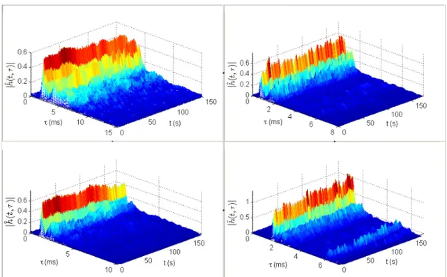
Figure 1: Examples of measured impulse responses

3. SLOW VS FAST FADING

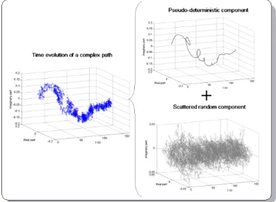
The observation of the measured impulse responses over 150 seconds suggests that signals propagating through an UAC are affected by fading phenomena of different scales. Fading is usually qualified as slow or fast to refer to the rate at which the magnitude and phase of the channel fluctuate compared to the transmission baudrate. Fast fading is predominant in the design of communication systems since the adaptive algorithms at reception must be tuned to its characteristics to ensure good performance. Slow fading is less critical as it represents only a long-term variation of the signal-to-noise ratio at reception. By looking at the envelope of the measured UACs (see Figure 2), it can be seen that the two fading types are combined in an additive way. The average value of the received power is time variant whereas the second order statistics on this received power seem to be invariant. On the observation window of 150 seconds, the UAC can therefore be considered as trend stationary and each path can be split up as:

) ( ) ( ) , ( ˆ _{t d t w t} h

τ

_k = _k + _k (1)

where d_k(t)is a pseudo-coherent component that behaves almost as if the medium was

deterministic and w_k(t) is the scattered random part. Note that d_k(t) can be considered as

pseudo-deterministic and hˆ(t,

τ

_k) as trend stationary only because the observation window

is time limited compared to the fluctuation speed of the underlying physical phenomena. A longer observation window may lead to different conclusions.

Figure 2: Time evolution examples of UAC path envelopes.

In order to isolate d_k(t) and w_k(t) from hˆ(t,

τ

_k), an empirical mode decomposition

(EMD) is performed on each path of the UAC. EMD is a method of signal decomposition, well suited to non stationary signals, that does not require any predetermined basis functions. The decomposition is designed to seek the different intrinsic modes of oscillations (or rotations in the complex case) in any data, based on the principle of local scale separation [5] [6]. Each path is then expressed as:

4 4 3 4 4 2 1 43 42 1 ) ( 1 , ) ( 1 0 , ( ) ( ) ( ) ) , ( ˆ t d N L i k k i t w L i k i k k k k k k t r t m t m t h

∑

∑

− = − = + + =

τ

₍₂₎

where m_i,k(t)is the i-th of theN modes, _k r_k(t) is the residue component and L is the _k

decomposition order used to separate d_k(t) and w_k(t). These two processes varying at

different paces (less than few seconds for w_k(t) and 10 seconds to several minutes for

) (t

d_k ), the choice of L is based on a frequency criterion on the path envelope. _k

4. STATISTICAL INFERENCE

Thanks to the EMD, it is now possible to study the characteristics of the two fading components independently. Since fast fading is more critical for communication system design than slow fading, we here only focus on the characterisation of the scattered

random components w_k(t). To model their probability density function (pdf), we applied

the principle of maximum entropy [7] constrained by some moments of different orders measured on the estimated impulse responses. Kullback-Leibler (KL) divergences between the model and the empirical pdf are then assessed for the tested moment orders.

Moment order 0 ≤ 1 ≤ 2 ≤ 3 ≤ 4 ≤ 5 ≤ 6

KL divergence 0.64 0.62 8.8 10−3 7.5 10−3 7.5 10−3 6.3 10−3 6.1 10−3

Table 1: Example of measured KL divergence for different constraints on the model

As illustrated in Table 1, the KL divergence converges as soon as the second order

constraint is applied to the model of maximum entropy. This indicates that the w_k(t) can

be well modelled by a stationary Gaussian process. This has been confirmed by a

Kolmogorov-Smirnov [8] test applied to the envelope of the w_k(t) that must follow, from

the model, a Rayleigh distribution. 96% of the tested paths pass the test with a significance

level greater than 5%. Consequently, each path hˆ(t,

τ

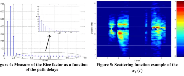
_k)can be modelled as a Rice process

with a slow time varying mean component. In addition, as shown in Figure 4, the power

ratio (Rice factor) between the mean component d_k(t)and the scattered part w_k(t) is

delay dependent and tends to zero (Rayleigh fading) for the most delayed paths. Note that the fluctuation period of the mean component being on the order of several thousands to hundreds of thousands symbols, the communication channel can be well approximated by a wide-sense stationary process.

Figure 4: Measure of the Rice factor as a function of the path delays

Figure 5: Scattering function example of the

) (t

w_k

To characterise into more details the fast fading components w_k(t), their coherence

time with 50% correlation have also been measured. All results obtained are within the

range of 300 to 600 ms. Figure 5 shows an example of the w_k(t) scattering function for a

5. ERGODIC CHANNEL CAPACITY

Ergodic capacity of a transmission channel is here considered since it provides a simple bound, independent of the actual signaling scheme and receiver algorithm. In underwater acoustic, at our best knowledge, this capacity has only been computed by modeling the UAC by a band-limited AWGN channel [12]. In agreement with the results found in the previous sections, the UAC, after removing long term slow fluctuations, is here modeled as a WSSUS [11] channel with a possibly non zero mean.

Applying same techniques as in [9], an upper bound can be derived for the ergodic capacity of this channel :

( )

(

)

        ⋅       + −         ₊ +

∫

− ≤ ≤

∫∫

≤

2 1 2 1 2 2 2 2 1 0 , 1 log 1 log Capacity

_Max

ν

τ

σ

τ

ν

β

β

α

ν

σ

ν

σ

α

α d d S d H w H w H

Here H(ν) stands for the Fourier transform of the mean of the channel response, ν is the

normalized frequency, σH2 the sum of the variance of all paths and SH(ν,τ) the scattering

function [11] (with reduced units ν, τ). The noise is assumed to be Gaussian, zero-mean

and i.i.d. with standard deviation σw (suchthat w N0W

2 ₌

σ

; W being the used bandwidth).

The input symbols sk are assumed to be zero-mean, i.i.d. and such that E{|sk|2}≤ 1 and |sk|2

≤ β (both average and peak transmitted power are limited).

It can be seen that the RHS of (3) is the sum of two terms: a first term which is the capacity of a AWGN channel (constant or time variable, but perfectly known) and a second term which is the capacity loss due to the unknown fluctuations of the channel. It is also worth noticing that maximization with respect to α of the expression (3) is simple when H(ν) is null or constant which corresponds to at most one non zero-mean path.

(a) R.TC/ = 10

(b) R.TC = 100

Figure 6: Channel capacity for a single path Rayleigh channel

A first example of the resulting bound on capacity is given Figure 6 in the case of a single path Rayleigh channel with Gaussian scattering function. The two different plots

correspond to two values of the coherence time TC the channel (in symbols); on each plot

the red curves correspond to different values of the Peak-to-Average Power Ratio (PAPR) β. Capacity of AWGN channel is also plotted (black curve) since it provides an upper bound of the channel capacity in any circumstances.

(3) C ap aci ty ( b it s/ sy m b ) C ap aci ty ( b it s/ sy m b ) SNRsymb (dB) β = 1 AWGN β = 2 β = 5 SNRsymb (dB) AWGN

It can be seen on this figure 6 that, for short coherence time Tc (R.TC =10 where R is

the symbol rate) the capacity is significantly lower than for the AWGN channel. For larger

coherence time TC (R.TC =10) the difference is smaller or even negligible. It also worth

noticing that for large value of R.TC the capacity bound (3) is maximized for α equal to 1

(transmitted power is averaged limited, constant modulus modulation as PSK). On the

contrary, for small values of R.TC, it is no more possible to use constant modulus

modulations (phase tracking becomes impossible) and incoherent spiky modulations, where information is carried by amplitude or epoch of spiky pulses, have to be used. For

small value of PAPR β, the parameter α then have to be taken lower than 1 and the

average power chosen lower than the maximum allowable.

(a) spreading factor ∆S = 0.1

(b) spreading factor ∆S = 0.01

Figure 7: Capacity of a WSSUS channel with a rectangular scattering function

A second example is given in Figure 7 for a WSSUS Rayleigh fading channel with a rectangular scattering function defined as

            ∆ = s s s H H T rect D rect S

ν

τ

σ

ν

τ

2 ) , ( ₍₄₎

where D and _s T are respectively the Doppler and time spread and _s ∆S is the spreading

factor, ∆S=D_sT . It can be shown in this particular case that the capacity only depends on _s

∆S, β and the SNR. Figure 7 indicates that the channel capacity is close to the AWGN

channel capacity for small spreading factor ∆S, but significantly lower for larger spreading

factor.

In practice, the acoustic channel analyzed in section 2-4 above corresponds to

favorable situations (spreading factor ∆S about 5.10-3 according to Figure 5), even more

favorable than the one on figure 6b-7b. Its ergodic capacity is therefore likely very close to the AWGN channel capacity. This is not always true since far more difficult UACs have

already been observed, with spreading factor ∆S up to 0.1 or higher, for which the channel

capacity vs SNR will be similar to figure 6a and 7a.

C ap aci ty ( b it s/ sy m b ) C ap aci ty ( b it s/ sy m b ) SNRsymb (dB) SNRsymb (dB) β = 1 AWGN β = 2 β = 5 AWGN

6. CONCLUSIONS AND PERSPECTIVES

A set of statistical tools and methods has been presented to characterize a given UAC as a transmission channel to then bound its capacity according to the outcomes of this characterization. These tools have here been applied to a first set of at sea data: the corresponding channel has been found in good agreement with a multipath Rayleigh or Rice fading channel with a small spreading factor and a capacity likely close to AWGN channel’s.

Further works will be devoted to the analysis of other at sea datasets corresponding to more difficult channels. During some experiments, data transmission has been found to be only possible with data rates far lower than the ergodic capacity of the corresponding AWGN channel. The aims of these analyses will then be to determine whether the transmission rate has been limited by “poor” signaling schemes and transmission algorithms or by the channel itself. In other respects, it would also be interesting to address the impulsive characteristics of the ambient noise and its consequence on the channel capacity.

7. ACKNOWLEDGEMENTS

The authors would like to thank the GESMA (Groupes d'Etudes Sous-Marines de l'Atlantique, Brest) for providing the raw data used for this work as well as Joël Trubuil for his fruitful collaboration.

REFERENCES

[1] B.S. Sharif, J. Neasham, O.R. Hinton and A.E. Adams, A computationally efficient Doppler compensation system for underwater acoustic communications, IEEE J. Oceanic Eng., Vol. 25, pp. 52-61, Jan., 2000.

[2] G. Eynard and C. Laot, Blind Doppler Compensation Techniques for single Carrier Digital Underwater Communications, OCEAN'S 2008, Québec, Canada, September 2008.

[3] H. Meyr, M. Moeneclaey and S. A. Fechtel, Digital Communications Receivers : Synchronization, Channel Estimation and Signal Processing, Wiley, 1998.

[4] P.A. van Walree, T. Jenserud and M. Smedsrud, A Discrete-Time Channel Simulator Driven by Measured Scattering Functions, IEEE JSAC, Vol. 26, no 9, December 2008.

[5] N.E. Huang, Z. Shen, S.R. Long, M.L. Wu, H.H. Shih, Q. Zheng, N.C. Yen, C.C. Tung, and H.H. Liu. The empirical mode decomposition and Hilbert spectrum

for nonlinear and nonstationary time series analysis. Proc. R. Soc. London A, 454:903–995, 1998. [6] G. Rilling, P. Flandrin, P. Gonçalves, and J.M. Lilly. Bivariate Empirical Mode Decomposition. IEEE Signal Processing Letters, 14(12):936–939, 2007.

[7] E.T. Jaynes, Information Theory and Statistical Mechanics. Physical review, 106(4):620–630, 1957. [8] M.A. Stephens, EDF Statistics for Goodness of Fit and Some Comparisons. Journal of the American Statistical Association, 69(347):730–737, 1974.

[9] T. Cover and J.A. Thomas, Elements of Information Theory, 2nd edition, Wiley & Sons, 2006

[10] G. Durisi, H. Bolcskei and S. Shamai, Capacity of Underspread Noncoherent WSSUS Fading Channel under Peak Signal Constraint, IEEE Int. Symposium on Information Theory (ISIT), Nice, France, pp. 156-160, June 2007

[11] P. Bello, Characterization of Randomly Time-Variant Linear Channels, IEEE transactions on Communications Systems, Vol. 11, N°4, December 1963, pp 360,393

[12] T.J. Hayward and T.C. Yang, Underwater Acoustic Communication Channel Capacity: A Simulation Study, High Frequency Ocean Acoustics Conference , Vol. 728, pp. 114-121, 2004