HAL Id: hal-01685414
https://hal.archives-ouvertes.fr/hal-01685414
Submitted on 6 Nov 2018
HAL is a multi-disciplinary open access
archive for the deposit and dissemination of
sci-entific research documents, whether they are
pub-lished or not. The documents may come from
teaching and research institutions in France or
abroad, or from public or private research centers.
L’archive ouverte pluridisciplinaire HAL, est
destinée au dépôt et à la diffusion de documents
scientifiques de niveau recherche, publiés ou non,
émanant des établissements d’enseignement et de
recherche français ou étrangers, des laboratoires
publics ou privés.
A decision support system for optimising the order
fulfilment process
Uche Okongwu, Matthieu Lauras, Lionel Dupont, Vérane Humez
To cite this version:
Uche Okongwu, Matthieu Lauras, Lionel Dupont, Vérane Humez. A decision support system for
optimising the order fulfilment process. Production Planning and Control, Taylor & Francis, 2012, 23
(8), pp.581-598. �10.1080/09537287.2011.566230�. �hal-01685414�
A decision support system for optimising the order fulfilment process
Uche Okongwua, Matthieu Laurasab*, Lionel Dupontband Ve´rane Humezb
aDepartment of Industrial Organisation, Logistics and Technology, Universite´ de Toulouse, Toulouse Business School,
20 Boulevard Lascrosses, 31068 Toulouse Cedex 7, France;bDepartment of Industrial Engineering, Universite´ de Toulouse, Mines Albi, Route de Teillet, 81013 Albi Cedex 9, France
Many authors have highlighted gaps at the interfaces between supply chains (SCs) and demand chains. Generally, the latter tends primarily to be ‘agile’ by maximising effectiveness and responsiveness while the former tends to be ‘lean’ by maximising efficiency. When, in the SC, disruptions (that lead to stock-out situations) occur after customer orders have been accepted, managers are faced with the problem of maximising customer satisfaction while taking into consideration the conflicting objectives of the supply and demand sides of the order fulfilment process. This article proposes a cross-functional multi-criteria decision-making (advanced available-to-promise) tool that provides different strategic options from which a solution can be chosen. It also proposes a performance measurement system to support the decision-making and improvement process. The results of some experimental tests show that the model enables to make strategic decisions on the degree of flexibility required to achieve the desired level of customer service.
Keywords: supply chain; demand chain; advanced available-to-promise; order fulfilment process; agility; lean
1. Introduction
In today’s highly globalised economy and competitive environment, most businesses are market-driven. Firms therefore look for new concepts, techniques and tools that would enable them to manage their demand and supply chains (SCs) in order to improve customer satisfaction, competitiveness and profitabil-ity. Customer satisfaction would lead to customer loyalty, which is one of the factors necessary to guarantee the sustainability of any business. In order to guarantee sustainable growth, companies aim to keep existing customers while gaining new ones. To do this, they do not have to be highly competitive only on cost and quality, but also on the reliability and speed of delivering customer orders. The order fulfilment pro-cess (OFP) is therefore one of the most important processes within an organisation and is considered by Lin and Shaw (1998) as one of the three pillars of a company, the other two being the product develop-ment process and the customer service process.
Croxton et al. (2001) break the OFP into two components: the strategic process, which ‘considers the manufacturing, logistics and marketing requirements necessary to design the distribution network’ and the operational process, which ‘defines the specific steps related to the way customer orders are generated and communicated, recorded, processed, documented,
picked, delivered, and handled after delivery’. This article develops a model that enables to measure the performance of the operational process, on the basis of which decisions can be made in order to improve the strategic process. Though not explicit in the activities described by Lin and Shaw (1998) and Croxton et al. (2001), the OFP can be broken down into two phases: . The first phase comprises the order promising activity (also referred to as ‘availability check’), which verifies the availability of resources in order to promise to the customer a given quantity that will be delivered on a given date. Readers interested in the details of this phase should refer to the work done by Chen et al. (2008).
. The second phase comprises the execution (or order fulfilment) activity, where the order is actually delivered as promised.
In an ideal situation, customer orders would be delivered as promised. In reality, operational disrup-tions such as machine breakdowns, material shortage and quality defects can lead to stock-out situations. If these disruptions occur at the first phase, then some of the customer orders may simply not be accepted. But, if they occur at the second phase, then some of the already accepted customer orders may not be fulfilled.
This article considers the second phase of the OFP and looks at how best already accepted customer orders can be fulfilled in stock-out situations. This entails developing a decision-making tool as well as a set of indicators to measure and improve the performance of the OFP. Within the OFP, the order management (OM) activity consists in analysing orders and manag-ing backlog in order to determine if, how and when orders can be delivered. Its main objectives are two dimensional (Lin and Shaw 1998):
. delivering qualified products to fulfil customer orders at the right time and right place; . achieving agility to handle uncertainties from
internal or external environments.
In practice, there are techniques that enable the OM activity to partly achieve these goals by choosing between different alternatives. As they will be discussed in Section, these techniques are available-to-promise (ATP), advanced available-to-promise (AATP), cap-able-to-promise (CTP) and profitable-to-promise (PTP). However, in the case of stock-out, they are insufficient for decision making in the face of certain variables such as unknown availability, product sub-stitution and specific operations.
An OFP involves generating, filling, delivering and servicing customer orders (Croxton 2003). It is a complex process because it is composed of several activities, executed by different functional entities, and heavily interdependent among the tasks, resources and entities involved in the process (Lin and Shaw 1998). Even though it has a clear global objective to provide to the customer the right product, at the right time, at the right place at the right price, each functional entity that participates in this process generally tries to achieve their own individual objectives. These objec-tives are often antagonistic. For example, in the case of stock-out, distribution may prefer to ship everything in one batch on a later date; the sales department may want to send backorders separately; marketing may not want to sell some products separately; manufactur-ing may not want to change their schedule; and of course, the customer would want to be delivered as promised.
This article therefore also aims to look at how the conflicting objectives of the different functional entities can be taken into consideration in the decision support system that is used to manage the OFP.
In the following section, we will discuss the literature concerning decision support systems used to support the OFP. We will go on to develop and discuss the set of indicators that will be used to measure the performance of the OFP based on our model. Then, our advanced ATP model is described
and applied to a practical case. Finally, we will discuss the results, before drawing some conclusions that will include perspectives for further research.
2. Decision support systems
2.1. Conventional order fulfilment techniques
There are several techniques that support the OFP and more precisely the OM activity. The most commonly used is probably ATP. In the 11th edition of the APICS dictionary (2005), the American Production and Inventory Control Society defined ATP as ‘the uncommitted portion of a company’s inventory and planned production maintained in the master produc-tion schedule to support customer order promising’. This promising mechanism is suitable for make-to-stock (MTS) production systems where finished goods (FG) are produced based on demand forecast and kept in inventory before orders are received from customers. In make-to-order (MTO), as well as in assemble-to-order (ATO) and engineer-to-assemble-to-order (ETO) strategies, delivery dates have to be set based on available capacity and material constraints in order to avoid ‘over promising’ and ‘under promising’ on job orders. Techniques used to achieve this goal are referred to as CTP.
A third technique, referred to as PTP, is used when profitability is taken into consideration in addition to capacity and material constraints. Kirche et al. (2005) define PTP as ‘the ability to respond to a customer order by determining how profitable it is to accept this order’. The analysis of a PTP system allows the business to find out if a particular order will be profitable to make, considering the raw material costs, process costs, inventory costs and other costs against the price the customer is willing to pay. In the case of MTS, PTP works on the data from distribution planning, while in the case of ATO, MTO and ETO, it works on the data from production planning.
This article deals with an MTS strategy, where the customer is delivered from FG inventory and sched-uled production.
As pointed out by Chen et al. (2002), ATP consists in simply monitoring the uncommitted portion of current and future available FG. Note that if no promise can be found for an order, the SC will not be able to fulfil the order within the allocation planning horizon (Kilger and Schneeweiss 2000). It is therefore more or less static. In Section 1, we mentioned that the OFP is composed of two phases: order promising and order fulfilment, ATP techniques are mostly used for the first phase, as described by Xiong et al. (2006).
This article looks essentially at the order fulfilment phase. In other words, the issue is: what happens when orders have been promised, but the available quantities are not sufficient to fulfil these orders in the right quantities and at the promised due dates?
2.2. Advanced order fulfilment techniques
Given the limitations of ATP models, some authors have proposed to develop AATP models in order to enhance the responsiveness of order promising and the reliability of order fulfilment (Pibernik 2005). Chen et al. (2002) define AATP as ‘a decision-making mechanism that can dynamically handle the uncertainty and unanticipated changes related to suppliers and customers, as well as production processes’. In other words, AATP directly links available resources (i.e. raw materials, FG and work-in-progress) as well as produc-tion and distribuproduc-tion capacities with customer orders in order to improve overall performance by bridging the gap between the forecast-driven SC and the order-driven demand chain (DC). Two characteristics used by Pibernik (2005) to classify AATP models are:
. the availability level: FG inventory or supply chain resources (SCR; materials and capacity); . the operating mode: real time (RT; orders are processed as they arrive) or batch mode (orders are received over a given time window and processed together).
Four AATP types are derived from these two characteristics as given in Table 1. These are: RT/FG, RT/SCR, batch time (BT)/FG and BT/SCR.
For each of these types, conventional ATP func-tionalities are searched along three dimensions: time, customer and product. Some additional advanced ATP functionalities are currently discussed by researchers (Kilger and Schneeweiss 2000, Pibernik 2005). They refer mainly to strategies applied to an anticipated shortage of FG or SCR. Based on these functionalities, three different strategies can be supported by AATP
models (Kilger and Schneeweiss 2000, Pibernik 2005, Siala et al. 2006):
. AATP with substitute products: in certain cases substitute products can be delivered within the given delivery time window in place of the product originally ordered by the customer;
. Multi-location AATP: if the customer order cannot be fulfilled with the FG or SCR in a given location, available FG and resources can be sourced from other locations;
. AATP with partial delivery: if the ordered quantity is not available within the given delivery time window, the customer order can be fulfilled with two or more partial deliveries. In the AATP planning mechanism, these different strategies can be combined in any possible sequence or in such a way that all feasible solutions are determined and assessed simultaneously (Pibernik 2005).
Some authors have attempted to develop models considering one or two of the four AATP types (Table 1), as well as none or just one of the three strategies mentioned above. For example, Chen et al. (2002) developed a BT/SCR AATP model and consid-ered two strategies (substitute raw materials and multi-sources). Pibernik (2005) presented two AATP types (RT/FG and BT/FG) using an optimisation approach and took only one strategy (partial delivery) into account. Siala et al. (2006) proposed a multi-location RT/FG AATP model that also considers substitute products. Pibernik (2006) presented a RT/FG AATP model for a single product.
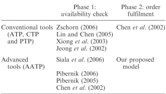
No author seems to have developed a model that simultaneously considers all three strategies (product substitution, partial delivery and multi-location sourc-ing). This is what we try to achieve in this article. Table 2 positions the contribution of this article with respect to the two phases of the OFP, as well as to the
Table 2. Decision-making tools classified according to the OFP phase. Phase 1: availability check Phase 2: order fulfilment Conventional tools (ATP, CTP and PTP)
Zschorn (2006) Chen et al. (2002) Lin and Chen (2005)
Xiong et al. (2003) Jeong et al. (2002) Advanced
tools (AATP)
Siala et al. (2006) Our proposed model Pibernik (2006)
Pibernik (2005) Chen et al. (2002) Table 1. Types of AATP models.
Operating mode
Availability level
FG SCR
RT RT/FG RT/SCR
BT BT/FG BT/SCR
Source: Adapted from Pibernik (2005).
Notes: FG, finished goods; SCR, supply chain resources; RT, real time and BT, batch time.
work of other authors. Moreover, none has studied the impact of the different functional entities involved in the OFP. In other words, the models of the above-mentioned authors consider essentially a single stake-holder’s point of view, that of the customer (Pibernik 2005) or that of the distribution centre (Siala et al. 2006). This article tries to bridge the gap between the conflicting objectives of the two sides.
We would like the reader to note that the acronym AATP is also used for allocated ATP by some authors such as Lee et al. (2006) and Herbert (2009). These are ATP systems that enable materials in short supply to be assigned to customer segments according to a pre-determined allocation policy. This is not the definition of AATP adopted in this article.
3. Performance measurement system
Some authors (Bourne et al. 2003, Chan et al. 2006) have reviewed the frameworks for developing and implementing a performance measurement system. Examples are Balanced Scorecard (Kaplan and Norton 1996), Activity Based Costing/Management (Cokins 1989), Supply Chain Operations Reference (Supply Chain Council 2008), Performance Prism (Neely et al. 2002) or ECOGRAI (Ducq and Vallespir 2005). This article does not intend to review these methods but simply to adopt one of them and use it to structure the development of performance indica-tors for the application of our model.
In this article, we have adopted the ECOGRAI method because it explicitly shows the link between the performance indicators and the decision variables. It is composed of six steps (Ducq and Vallespir 2005). Step 1 consists in modelling the control and controlled structures. The aim is to determine the physical system for which the performance will be analysed, as well as the decision centres of the management system in which the decisions are made to control and improve the performance. Step 2 aims to identify the objectives of the decision centres identified. Step 3 consists in identifying the decision variables that correspond to each objective of the decision centres. In step 4, the performance indicators are defined. An information system for the performance indicators is designed in step 5 and its integration into the company’s informa-tion system is done in step 6. In this article, only steps 1–4 are presented.
3.1. Modelling the control structure
Most firms aim to manage both their DC and their SC such as to: (1) maximise the satisfaction of the ultimate
customer by delivering quickly and responsively error-free products at a relatively low price, and (2) minimise operational cost by eliminating non-value-added activ-ities and reducing lead times, thereby creating value for stakeholders. Christopher (1992) defined a SC as ‘the network of organisations that are involved, through upstream and downstream linkages, in the different processes and activities that produce value in the form of products and services delivered to the ultimate consumer’. The downstream linkages constitute the DC, which is defined by Hoover et al. (2001) as ‘the chain of activities that communicate demand from markets to suppliers’. From this definition, the SC can be referred to as the upstream linkages, which encom-pass all the activities involved in fulfilling the demand by supplying products and/or services to the market.
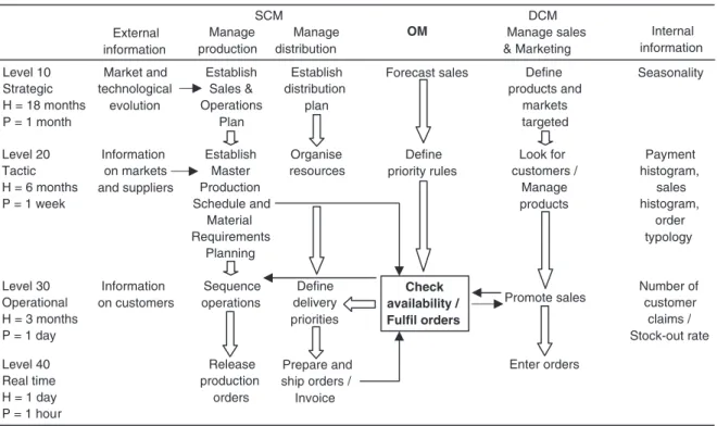
The integration of the SC and DC processes entails developing the communication, co-operation and coordination capabilities of the functional entities involved. To achieve this, the OFP and more precisely the OM activity has to be executed properly. Figure 1 shows the ECOGRAI control structure, which identi-fies the key functions involved in the OFP. Vertically, this structure clearly shows the activities of each function at different horizons (strategic, tactical and operational) and the relationship between the functions can be seen horizontally.
The OM function serves as a ‘bridge’ between the SC and the DC and highlights the availability check/ order fulfilment decision centre, which constitutes the central axis in this article.
3.2. Objectives of decision centres
Though there are different definitions of demand chain management (DCM) and supply chain management (SCM) in the literature, some authors argue that SCM is termed DCM to reflect the fact that the chain (or network) is driven by the market, and not by suppliers (Rainbird 2004). It could be said that SCM lays emphasis on efficiency (which consists in minimising operational cost) while DCM lays emphasis on effec-tiveness (which consists in maximising flexibility and responsiveness), but tries more to reconcile both efficiency and effectiveness (Walters 2006a). It follows that the decision centres on the supply side of the OM activity would aim to be ‘lean’ (efficient) by eliminating wastes while those on the demand side would aim to be ‘agile’ (flexible and responsive) by providing speedy response to market changes. A firm is best placed to create value and exploit market opportunities when there is an effective combination of SC capabilities (efficiency) and DC effectiveness to maximise the
organisation’s overall value chain (Walters and Rainbird 2004). This is the role of the OM activity as it is positioned in Figure 1.
Being at the intersection of the SC and the DC, the OM activity searches for an optimal solution and would aim to be lean and agile at the same time. This calls for a ‘leagile’ system. Naylor et al. (1999) defined leagility as: ‘the combination of the lean and agile paradigms within a total SC strategy by positioning the customer order decoupling point so as to best suit the need for responding to a volatile demand downstream yet providing level scheduling upstream from the decoupling point’. The objectives of the decision centres are therefore oriented towards leanness, agility and leagility.
3.3. Performance dimensions
Johansson et al. (1993) developed a conceptual model that would help to understand and manage the leagility concept. Their model, taken further by other authors (Childerhouse and Towill 2000, Christopher and Towill 2000), expresses the value delivery of a business in terms of an equation which encompasses market qualifiers and market winners, as follows:
Total value¼quality" service
cost" lead time: ð1Þ
In this equation, cost is a market winner for a lean system while customer service level is a market winner for an agile system. Given that quality and lead time are market qualifiers for both lean and agile systems, if we consider that efficiency is inversely proportional to cost (i.e. efficiency increases as cost decreases) and that effectiveness and responsiveness are directly propor-tional to customer service level (i.e. customer service level increases as effectiveness and responsiveness increase), then Equation (1) can conceptually be rewritten as
Total value¼ efficiency " effectiveness
" responsiveness: ð2Þ
These elements, efficiency, effectiveness and responsiveness, constitute the three primary perfor-mance dimensions of our study. The lean objective can be achieved by increasing the efficiency of the SC decision centres, while the agile objective can be achieved by increasing the effectiveness and/or respon-siveness of the DC decision centres. Partial or total leagility can be achieved by partially or totally com-bining the three dimensions. Figure 2 shows our performance framework (the three primary perfor-mance dimensions, as well as what we could refer to
as secondary performance dimensions, which
are derived from various combinations of the
SCM DCM
Internal information
OM
Manage Manage Manage sales External
information production distribution & Marketing
H = Horizon and P = Period Level 10 Market and
technological evolution Establish Sales & Operations Plan Establish distribution plan Define products and markets targeted
Forecast sales Seasonality Strategic H = 18 months P = 1 month Information on markets and suppliers Establish Master Production Schedule and Material Requirements Planning Define priority rules Organise resources Level 20 Tactic H = 6 months P = 1 week Look for customers / Manage products Payment histogram, sales histogram, order typology Level 30 Operational H = 3 months P = 1 day Information on customers Sequence operations Define delivery priorities Number of customer claims / Stock-out rate Check availability / Fulfil orders Promote sales Release production orders Prepare and ship orders / Invoice Enter orders Level 40 Real time H = 1 day P = 1 hour
primary dimensions). The secondary dimensions are: total agility (effectiveness, responsiveness and flexibil-ity); partial effective leagility (efficiency, effectiveness and flexibility); partial responsive leagility (efficiency, responsiveness and flexibility) and total leagility (effi-ciency, effectiveness, responsiveness and flexibility).
3.4. From performance dimensions to performance indicators
Indicators are needed to measure the performance dimensions (efficiency, effectiveness and responsive-ness) that we mentioned in Section 3.3. Many authors (Holweg 2005, Walters 2006b, Reichhart and Holweg 2007, Stevenson and Spring 2007, Zokaei and Hines 2007) have emphasised the vagueness, the multidimen-sionality and the interdependency in the definitions of these performance dimensions, which sometimes make them difficult to measure in practice. We do not intend to review the literature of these terms, but simply to adopt a strict and clear definition of each of them, such as to be able to define the various strategies that will be used in our AATP model. We will adopt the following restrictive and 1-D (or single factor) definitions:
. Efficiency is doing things right (Zokaei and Hines 2007) and this can be defined as the cost of fulfilling customer orders. Although effi-ciency is generally measured with respect to the best possible way of doing something, some authors define it in relative terms as the best of all possible ways of doing something (Bescos and Dobler 1995, Mas-Colell et al. 1995, Halley and Guilhon 1997). Some of
these authors go further to suggest that it can best be measured in financial terms in order to reflect the primary goal of profit-making organisations. Walters (2006b) suggests that efficiency should be measured from a broad perspective that encompasses customer needs, rather than from a narrow perspective that considers only the supply’s short-term cost reduction objectives. Therefore, if we consider the OFP as being composed of the following elements: order preparation, transportation, substitution, delay, shortage (undelivered quantity), efficiency can be measured as the total cost of the five elements, expressed simply in financial values.
. Effectiveness is doing the right thing (Zokaei and Hines 2007) and this can be defined as fulfilling orders exactly as they are requested by customers (i.e. the completeness of cus-tomer orders). It is measured in terms of the percentage of the order that is fulfilled within the time frame that is acceptable by the customer. Its value can go from 0% to 100%, the latter being the best. Zero per cent means that nothing is delivered within the time frame acceptable by the customer and 100% means that all the ordered quantity was delivered within the acceptable time frame, with or without substitute products. This performance criterion is the ‘completeness percentage’.
. Responsiveness is doing things quickly and this can be defined as the speed at which customer
Efficiency x Total leagility (x, y, z) Effectiveness z Partial leagility (x, y) Partial leagility (x, z) Total agility (y, z)
Partial agility (y) L e a n (x) Pa r t i al ag i l i ty (z) Responsivenessy
orders are fulfilled. We propose to measure it as the normalised average delivery time (NADT) of the total quantity that is delivered. For example, if a customer places an order for 200 units of a product, to be delivered in week 1 (due date) and accepts that the order be delivered within a maximum time of 4 weeks beyond the due date. If 80 units are delivered in week 1, 60 in week 2, 30 in week 3, 10 in week 4, and 20 in week 5, responsiveness is equal to 0.71. This is obtained by calculating the NADT as follows:
NADT¼ ½ð80 " 1Þ þ ð60 " 0:75Þ þ ð30 " 0:5Þ þ ð10 " 0:25Þ þ ð20 " 0Þ'=200 ¼ 0:71: In this example, since the maximum acceptable lateness after the due date is 4 weeks, each week of delay after the due date corresponds to a factor of 0.25 (i.e. ¼). This is why the 60 units delivered in week 2, with a delay of 1 week, are multiplied by 0.75 (i.e. 1( 0.25), the 30 units delivered in week 3 are multiplied by 0.5 (i.e. 1( 0.5), the 10 units delivered in week 4 are multiplied by 0.25 (i.e. 1 ( 0.75) and the 20 units delivered in week 5 are multiplied by 0 (i.e. 1( 1). Of course, the 80 units delivered on time in week 1 are multiplied by 1 (i.e. 1( 0). Being normalised, the value of responsiveness must be between 0 and 1, the latter being the best. A value of 1 means that 100% of the ordered quantity was delivered on or before the due date; a value close to 1 implies that a high percentage of the ordered quantity was delivered on or before the due date and/or that most of the delivery was done (quickly) within the first period after the due date; while a value close to 0 implies that most of the delivery was
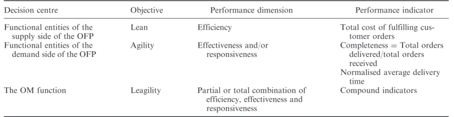
done (lately) within the last period of the acceptable time window after the due date. Flexibility is the range (number) of options available to do things and this can be defined as the range of options designed into the SC, which will enable it to fulfil customer orders. It is measured in terms of the number of substitutes for each product and the number of sites from which each product can be shipped (multi-site shipment). These flexibility elements should have a positive impact on effectiveness and respon-siveness and could have a positive impact on efficiency. A summary of the performance measurement system is presented in Table 3.
3.5. From performance dimensions to decision variables
In order to be able to implement the mathematical programming model that we will develop in Section 5, the performance dimensions described in Section 3.3 have to be translated into decision variables. If we consider that the SC/DC should aim to deliver the right quantity ordered by the customer, at the right time and at minimum cost, irrespective of possible changes (or disruptions) and risks embodied in the fulfilment process, then the performance dimensions can be translated into decision variables in the follow-ing way:
. Efficiency refers to the cost element and the decision variable is the overall cost of fulfilling an order.
. Effectiveness refers to the ‘right quantity’ element and the decision variable is the shortage component in our model.
. Responsiveness refers to the ‘right time’ ele-ment and the decision variable is the delay component.
Table 3. Summary of our performance measurement system.
Decision centre Objective Performance dimension Performance indicator Functional entities of the
supply side of the OFP
Lean Efficiency Total cost of fulfilling cus-tomer orders
Functional entities of the demand side of the OFP
Agility Effectiveness and/or responsiveness
Completeness¼ Total orders delivered/total orders received
Normalised average delivery time
The OM function Leagility Partial or total combination of efficiency, effectiveness and responsiveness
. Flexibility can be considered as the element that enables the system to adapt to changes and the decision variable is the substitution component.
We note that, in our model, all these variables will be expressed in terms of cost in order to facilitate the problem-solving process by using a common unit (that is relevant) to support the decision maker. In other words, our model calculates the cost of shortages and delays, and then tries to minimise them, with the aim of maximising the overall efficiency of the OFP. In this model, coefficients are used to vary the impact of the decision variables on the objective function in order to obtain and study different strategic configurations as will be discussed later in Section 5.2.
4. Research assumptions and hypotheses
In this section, we will describe the hypotheses of our model and the associated symbols used in it.
4.1. The customer
The first hypothesis considers that an order is com-posed of n different lines (multi-references order). Each line can be defined by a product p and a quantity Dp.
The product p is positioned on the line p.
The customer wants to be delivered at a due date, DD. There is a delay as soon as the effective delivery date is beyond the DD. The latest delivery date authorised by the customer is referred to as the deadline, DL. Beyond this DL, the customer will refuse the backorder. If not all ordered quantity is delivered, there is a shortage cost, CShp.
We also consider a delay cost, CDVp. This cost
depends on the laps of time between DD and the effective delivery date, as well as on the quantity delivered late. There is also a delay penalty, which is considered as a fixed cost, CDF.
An order can be delivered in several instalments. Nshipmax stands for the maximum number of ship-ments for an order. We consider that there are two shipments as soon as an order is delivered from two different sources s or prepared from a unique source but at two different dates.
Given that an order line p can be delivered in several instalments, Nsplitmaxp stands for the
maxi-mum number of splits authorised by the customer, for a given line. We consider that a line is split if and when the overall quantity of the line is delivered in several shipments. Two different cases must therefore be considered: the total quantity is shipped from a sole source at different dates or the total quantity is shipped
from different sources. No particular cost has been associated with this in order not to penalise the supplier twice. Actually, as soon as a line is split, the whole order will be delivered late (entailing therefore a delay cost) or delivered from different sources (entail-ing therefore an increase in the transportation cost).
4.2. Substitute products
In this study, we have envisaged the possibility of using a substitute product in place of the product in shortage. Consequently, the original product p can be substituted by a set of products Sp. We consider that P (group of demanded products) and S (group of substitute products) are disjoined. Then, let us consider Rr as the set of products ofP that r can replace. The cost of substitution (denoted by QSp) depends only on
the quantity of the substitute. We note that all products (original or substitute) can be delivered from different sources s.
4.3. Preparation and shipments
One shipment from a sourcing site s implies a preparation cost (CP) that includes a fixed part CPFs
(which depends on the sourcing site) and a variable part CPVpsthat depends also on the sourcing site, as well as on the quantity of product p picked.
A transportation cost is also considered. This cost is defined as a variable cost, CTVgsthat depends on the
weight of the quantity shipped and the distance between the sourcing site s and the customer. A product p gets a weight Wp. This cost is directly
proportional to the distance between the source and the customer. But since this article studies the case of only one customer, our model does not include any variable (index) c for customer. Therefore, for a given distance, the transportation cost is determined just for different weight brackets of the ordered quantity. Generally, there are two cases:
(1) A fixed cost for each weight bracket. For example, if the shipping cost of a quantity between 0 and 5 kg is 8 euros and that of a quantity between 5 and 10 kg is 10 euros, the shipping of a quantity of 6 kg and a quantity of 9 kg will both cost 10 euros.
(2) A degressive cost for each weight bracket. For example, if for a weight between 0 and 5 kg, the cost is 2 E/kg and for a weight between 5 and 10 kg, it is 1.5 E/kg, the shipping cost of a quantity of 6 kg will be 9 E (6" 1.5 E) and that of a quantity of 9 kg will be 13.5 E (9" 1.5 E).
In this case, transporters are encouraged to search for economy of scale.
In this study, we consider only the second option.
5. Proposed model 5.1. AATP model
Here, we define the elements used in our AATP model. The model is based on an OFP viewed from the receiving end rather than from the shipping end. The notations used as indexes, parameters and variables are summarised in Table 4. All variables are expressed with respect to the delivery date. In this case, pickup dates are equal to delivery dates minus lead times. Moreover, it is assumed that all picked-up quantities are delivered. As discussed in Section 3.5, the objective function (3) tries to minimise the total cost of the system (preparation costs CP, transportation costs CT, delay costs CD, substitution costs CS and shortage costs CSh). We propose to balance the different costs of the system in order to be able to reflect the strategy of the network. The aim is to minimise the total cost: Minimise½cðCPÞ ) CP þ cðCTÞ ) CT
þ cðCDÞ ) CD þ cðCSÞ ) CS þ cðCShÞ ) CSh', ð3Þ where c is the balancing coefficient for cost.
The different costs are defined below. Order preparation cost (CP):
CP¼X s X t DCUst ! ) CPFs þX p X s X t XpstþX i2Sp Yipst ! " # ) CPVps ð4Þ Transportation cost (CT):
Case 1: a fixed cost for each weight bracket
CT¼X t X s X g DELstg) CTVgs ð5:1Þ
Case 2: a degressive cost for each weight bracket
CT¼X t X s X g PFstg) CTVgs ð5:2Þ Delay cost (CD): CD¼ OD ) CDF þ X t¼DL t¼DD X p Qpt) CDVp) ðt ( DDÞ: ð6Þ Substitution cost (CS): CS¼X p QSp) CSVp: ð7Þ Shortage cost (CSh): CSh¼X p shortagep) CShp: ð8Þ
The above objective function is solved subject
to 22 constraint functions that are listed in
Table 5.
5.2. Implementing the order fulfilment strategies In our model, we have considered the OFP as being composed of the following decision variables: order preparation, transportation, substitution, delay and shortage (undelivered quantity). With respect to the principles described in Section 3.5, the performance
dimensions (delivery strategies) developed in
Section 3.3 can be implemented in the following way: (1) Efficiency: a similar coefficient should be put
on all the cost elements in the objective function stated in Equation (3), with the exception of the substitution cost (non-flexible condition), the objective being to minimise the global cost of the order fulfilment.
(2) Effectiveness: a higher coefficient should be put on shortage, the objective being to maximise the completeness of the orders by minimising shortages.
(3) Responsiveness: a higher coefficient is put on delay, the objective being to deliver as quickly as possible. In a way, quick delivery enables to minimise the risk of shortage. So, a medium coefficient could also be put on shortage. (4) Agility (effectiveness and responsiveness in a
flexible environment): a high coefficient is put on shortage (for effectiveness) and delay (for responsiveness).
(5) Partial effective leagility (efficiency and effec-tiveness in a flexible environment): a high coefficient is put on shortage (for effectiveness) and the coefficients put on order preparation, transportation, substitution and delay should be balanced (for efficiency).
(6) Partial responsive leagility (efficiency and responsiveness in a flexible environment): a high coefficient is put on delay (for responsive-ness) and the coefficients put on order prepa-ration, transportation, substitution and shortage should be balanced (for efficiency).
(7) Leagility (Efficiency, effectiveness and respon-siveness in a flexible environment): coefficients should be balanced between all the five elements.
These scenarios represent the extreme strategies derived from the conceptual framework presented in
Section 3.3 and do not constitute a complete experi-mental plan. In our future research, it will be interest-ing to study the impact of a larger panel of order fulfilment strategies.
We note that, since the cost elements of the objective function (Equation 3) are weighted using
Table 4. Indexes, parameters and variables of our model.
Notations Explanation
Indexes used in our model
p Product index, p¼ 1. . . n, n is the total number of lines in the order q All products (order or substitute)
r Substitute product (replacement product) index
s Source (distribution centre) index, s¼ 1. . . S, S is the number of sources t Time period index, t¼ 1, . . . , T, T is the planning horizon
g Weight bracket index, g¼ 1, . . . , G, G is the number of weight brackets Parameters of our model
ATPqst Quantity of product q that can be shipped from site s, between dates 1 and t
CDF Fixed penalty if there is a delay of at least one period within the order delivery time window (for DD5 t 5 DL)
CDVp Cost of delay for one period for product p (for DD5 t 5 DL)
CPFs Fixed preparation cost for site s
CPVqs Preparation cost for product q on site s
CShp Cost of shortage for product p
CSVp Cost of substitution for product p
CTVgs Transportation cost for a delivery within weight bracket g, from site s to customer
DD Due date
DL Deadline
Dp Demand of product p in a given order
kmaxg Superior limit of weight bracket g
kming Inferior limit of weight bracket g
Nshipmax Maximum number of shipments allowed
Nsplitmaxp Maximum number of splits allowed for a given order line p
RPr Set of products for which r can be a substitute
Sp Set of substitute products for product p
T Planning horizon
TLs Delivery time from site s to customer
Wq Weight of one product q
Variables of our model
DCUst Variable linked to the use of source s for a delivery on date t (distribution centre using),
DCUst¼ 1 if site s is used, 0 otherwise
DELstg Binary variable linked to weight bracket g of a delivery from site s on date t, DELstg¼ 1 if
there is a delivery within the weight bracket g from site s on date t, 0 otherwise
OD Binary variable linked to the due date (order delay), OD¼ 1 if there is a delay, 0 otherwise PEst Weight of the delivery sent from s on date t
PFstg Weight of the delivery within the weight bracket g. PEstg¼ PEstif DELstg¼ 1 PEstg¼ 0 if
DELstg¼ 0
ORpst Binary variable linked to the quantity of product delivered on date t from site s to fill line p
Qpt Quantity of product delivered on date t to fill line p (product p or substitute)
QSp Quantity of product p substituted
Rpst Quantity of product delivered on date t from site s to fill the line p (product p or substitute)
Shortagep Final backorder quantity of product p
XCpst Total quantity of product p picked on site s and delivered on date t
Xpst Quantity of product p picked on site s (on date t – DLs) and delivered on date t
XRCrst Total quantity of substitute product r picked on site s and delivered on date t
XRrst Quantity of substitute product r picked on site s and delivered on date t
Table 5. The constraint functions of our model.
Definition Equation
Equation number Sum of the different cost balancing coefficients must be
equal to 1
c (CP)þ c (CT) þ c (CD) þ c (CS) þ c (CSh) ¼ 1 (9) The quantity of product p delivered on date t (t5 DL)
must be equal to the total of product p or substitute product r delivered from all sourcing sites s
Qpt¼P s
Rpst for t* DL (10)
The customer does not allow any deliveries after the date DL
Qpt¼ 0 if t 4 DL (11)
Quantity of product p arriving from each sourcing site s at each date t
Rpst¼ Xpstþ P r2Sp
Yrpst for t* DL (12)
The total quantity of product p delivered from source s at date t must be lower than or equal to the quantity available at this source s at the shipment date (t – DLs).
ATP corresponds to a cumulative quantity of products available at a date t irrespective of the quantity XCpst of products picked up at t-DLs
XCpst¼ P i¼1,t
Xpsi (13)
XCpst* ATPpst-DLs for t4 DLs (14)
Example: If ATP111¼ 5, ATP112¼ 12 and ATP113¼ 16,
then it is possible to pick up: x products at t¼ 1 with x* 5; y products at t ¼ 2 with y * 12 ( x; z products at t¼ 3 with z * 16 ( y
The quantity of product p delivered from source s at date t is equal to 0, if t is lower than or equal to the delivery time from the site s
Xpst¼ 0 for t * DLs (15)
These are similar constraints (as in Equation (14)) for substitute products XRrst¼ P i2R Pr Yipst (16) XRCrst¼ P i¼1,t XRrsi (17) XRCrst* ATPrst(DLs for t4 DLs (18) XRrst¼ 0 for t * DLs (19)
Within the whole time window, the quantity of product p substituted is equal to the sum of the quantity of product r substituted to p QSp¼ P r2Sp P s P t Yrpst (20)
The shortage is equal to the total quantity ordered minus the total quantity delivered at date DL
P
t
Qptþ Shortagep¼ Dp8p (21)
For a given order, a sourcing site must be used less than the maximum number of shipments acceptable for the order Nshipmax+P s P t DCUst (22)
Each time a sourcing site is used (DCUst¼ 1), the
quantity of product delivered is limited by the total demand of p (for each product and each distribution centre). Thus if DCUs¼ 0 (an unused source s), then
Qpt¼ 0
XpstþP i2Sp
Yipst* Dp) DCUst 8p, 8s, 8t (23)
The number of pickings to fill a given order line p is limited by the maximum number of splits acceptable by the customer. Because one split implies two shipments, we have to consider ORpst( 1
Nsplitmaxp+P s
P
t
ORpst( 1 (24)
If the sourcing site s is used to deliver the order line p at period t (Rpst4 0), then ORpst¼ 1
Rpst* Dp) ORpst 8p, 8s, 8t (25)
Weight of the delivery sent from s on date t PEst¼P p Wp) Xpstþ WrP r2Sp Yrpst ! (26) A delivery must be done in only one weight bracket P
g
DELstg¼ 1 (27)
PEst¼P g
PEstg (28)
The weight of the delivery must fall between the limits of the weight bracket
kming) DELstg* PEstg5 kmaxg) DELstg (29)
The binary variable OD linked to the due date must be equal to 1 if at least one product is delayed
P t¼DL t¼DD P p Qpt* OD )P p Dp (30)
coefficients, the total cost does not correspond to the real logistics cost. Indeed, our model being a decision-making tool that aims to find a trade-off between the different performance dimensions (efficiency, effective-ness and responsiveeffective-ness), the difference between the real logistics cost and the total cost of the objective function can be regarded, from a strategic decision-making point of view, as a trade-off cost. Slack and Lewis (2008) define trade-offs in operations as the way firms are willing to sacrifice one performance objective to achieve excellence in another. From the strategic cost management perspective, this trade-off cost could be referred to as a structural or executional cost that enables the firm to minimise the negative impact of the actions of one business function on another business function (Anderson and Dekker 2009a,b). Logue (1975) argues that, in the assessment of market efficiency, the chief cost of dealing with a market-maker is the difference between the theoretical but unobservable equilibrium price and the transaction price. In a similar way, we therefore argue that the difference between the real logistics cost and the objective function cost (which is the equilibrium cost) corresponds to the strategic price that the firm has to pay in order to maximise (or optimise) the customer’s satisfaction.
6. Numerical application 6.1. Presentation
We carried out two experiments, which enabled us to test on the one hand non-flexible strategies (efficiency, effectiveness and responsiveness) and on the other hand, flexible strategies (total agility, partial effective leagility, partial responsive leagility and total leagility). For the non-flexible strategies, substitution and multi-sourcing capabilities are not taken into consideration while for the flexible strategies, flexibility is added to the system by allowing the substitution of products and by using a second sourcing site.
Each strategy is implemented using a set of values relative to the five cost balancing coefficients – c(CP), c(CT), c(CD), c(CS) and c(CSh). Based on the perfor-mance framework that we proposed in Section 3.3 and using the values of the three performance indicators: NADT (responsiveness), total cost (efficiency) and completeness (Effectiveness), the results obtained are expressed in the form of a 3-D surface graphical presentation (see the figures in the discussions that follow). Each result is represented by a point with coordinates as NADT, total cost (normalised in order to obtain a value between [0;1]) and completeness.
We consider an order placed by a customer at t¼ 0. This order is composed of three different products – M, N and O – and the demand is 100 units for each. The due date is week 1. But in week 1, there is a shortage of all these products. The customer does not want to receive his order in more than three instal-ments and the order line of product M cannot be split more than once. The latest delivery date acceptable by the customer is week 5. The set of data used to perform the first experiment (without flexibility) is shown in Table 6.
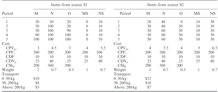
Regarding the second experiment, products MS and NS are added as substitutes for products M and N, respectively. In addition, a second sourcing plan S2 is opened and some inventories (for all the products) are introduced. The set of data used to perform this second experiment (with flexibility) is shown in Table 7. We assume that all products shipped in a given week are delivered the same week.
6.2. Results and discussion of experiment 1
Given the absence of flexibility, the coefficient c(CS) is equal to 0 (no substitution). All the results are shown in Figure 3.
As discussed in Section 3, the efficiency strategy is based on the minimisation of the total cost. The solution obtained turns out to be the most economic, with a total cost of $17160. The efficiency objective is clearly illustrated by the fact that the delivery plan includes in week 1, a quantity of 18 units of product O (and not the 20 units available) such as to benefit from a lower transportation cost in week 2. Actually, the
Table 6. Data for experiment 1 of the single-order case. Items from source S1
M N O Price $100 $160 $100 Period 1 50 30 20 2 50 100 20 3 50 100 90 4 90 100 100 5 100 100 100 Cost CPVps 3 4.5 3 CPFs 200 200 200 CDF 10 10 10 CDVp 25 40 25 CShp 200 360 200 Weight 1 0.7 0.5
two units of product O that are added to the 70 units of product N allow the weight group to be changed from [0, 50] to [50, 200], thereby minimising the total cost.
In line with its aim to maximise the completeness percentage of the customer order, the effectiveness strategy gives a delivery plan that enables to deliver all the products within the time window of 5 weeks
Figure 3. Results of experiment 1 of the single-order case. Table 7. Data for experiment 2 of the single-order case.
Items from source S1 Items from source S2
Period M N O MS NS Period M N O MS NS 1 50 30 20 0 10 1 20 40 0 10 30 2 50 100 20 0 10 2 30 40 50 10 30 3 50 100 90 0 10 3 50 60 50 10 30 4 90 100 100 0 10 4 50 60 50 10 30 5 100 100 100 0 10 5 50 60 50 10 30 Cost Cost CPVps 3 4.5 3 4 5.5 CPVps 4 5.5 4 5 6.5 CPFs 200 200 200 200 200 CPFs 200 200 200 200 200 CDF 10 10 10 10 10 CDF 10 10 10 10 10 CDVp 25 40 25 25 40 CDVp 25 40 25 25 40 CShp 200 360 200 CShp 200 360 200 Weight 1 0.7 0.5 1 0.7 Weight 1 0.7 0.5 1 0.7 Transport Transport 0–50 kg $10 0–50 kg $12 50–200 kg $8 50–200 kg $10 Above 200 kg $5 Above 200 kg $7
acceptable by the customer. However, compared to the efficiency strategy, the relatively small improvement (4%) in completeness might not be sufficient to compensate for the 8% increase in total cost and the 7% decrease in NADT.
The responsiveness strategy implies quickness and aims to deliver all the ordered quantity as soon as the products are available. This strategy enables to obtain the solution with the best NADT value – all the products are shipped within 3 weeks whereas in the other two strategies (efficiency and effectiveness) 4 and 5 weeks are, respectively, required to fulfil the order. Here again, this strategy would be adopted only in exceptional cases since, compared to the other two strategies, the relatively small improvement (5% and 12.5% with respect to efficiency and effectiveness, respectively) in NADT may not counterbalance the large increase (24% and 15%, respectively) in total cost, as well as the decrease (16% and 20%, respec-tively) in completeness.
In this experiment, the efficiency strategy turns out to be outstanding compared to the effectiveness and responsiveness strategies. This is however understand-able given the absence of flexibility (only one sourcing site and no substitutes products). Nevertheless, these two strategies can be adopted under specific circum-stances where the quickness and completeness of the delivery of the customer order is much more important than the cost of delivering the order. For example, in the healthcare industry, a hospital (the customer) will most likely want its order of certain medication to be delivered quickly and completely at a higher cost if that will enable to save the life of a patient suffering from chronic cancer. We can therefore say that the results of this experiment enable us to emphasise two interesting aspects of our model. Firstly, by assigning different balancing coefficients to the different components of an OFP, the total cost of the OFP can be minimised while meeting the contractually agreed requirements of the customer. Secondly, by varying the balancing coefficients, the supplier can modulate the different performance objectives (efficiency, effectiveness and responsiveness) in order to adapt to the customer’s expectations at different times and under specific circumstances. In other words, the supplier can constantly adapt its strategy depending on the market contextual conditions and requirements.
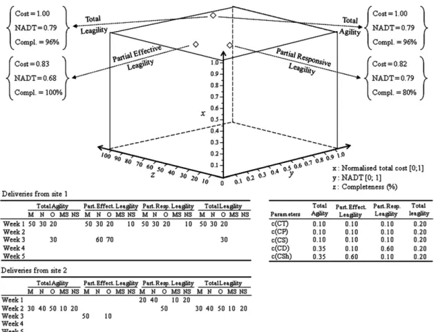
6.3. Results and discussion of experiment 2
All the solutions of this experiment make use of the flexibility capabilities of the supply network: two
sourcing sites and substitute products. The results are shown in Figure 4.
The leagility strategies give some relevant results. In line with its primary goal, the partial effective leagility strategy produces an interesting compromise in that it maximises effectiveness (with completeness equal to 100%) and provides a good efficiency value (with total cost equal to $15,010, which is better than that obtained in the three strategies studied in the first experiment) at the expense of responsiveness (with NADT equal to 0.68). Similarly, the partial responsive leagility strategy gives the best responsiveness (with NADT equal to 0.79) and an equally good efficiency value (with total cost equal to $15,144), while effec-tiveness drops significantly to 80%. The total leagility strategy looks for a compromise between the three variables. This explains why, compared to the two partial leagility strategies, the total cost ($12,424) is lower and therefore better, the value of NADT (0.79) is just as good as that of the partial responsive leagility strategy, while the value of completeness (96%) is between the two strategies. Generally, we note that the total leagility strategy constitutes an option better than the two partial strategies. However, in a situation where completeness is the customer’s primary require-ment, the partial effective leagility strategy might be a better option, though with the data used in this experiment, the difference between the values of completeness is relatively small.
Regarding the total agility strategy, it basically entails penalising delay and shortage in order to obtain a solution (an order fulfilment) that maximises effec-tiveness and responsiveness. Ideally, compared to the total leagility strategy, this strategy should generate either better values of NADT and completeness or a worse value of efficiency given that the total leagility strategy looks for a compromise between the three variables. Surprisingly, the results of these two strat-egies are exactly the same. This is probably not only due to the nature and composition of the data file that we used, but also to the very low level of flexibility (only one additional sourcing site, one substitute product and few inventory) incorporated into the supply network. Moreover, as in real life, the problem studied in this experiment includes a strong constraint imposed by the customer, that is, product M cannot be split more than once. By relaxing this constraint, we observed an improvement in the effectiveness and responsiveness of the total agility strategy, while the efficiency component decreased. Following this discus-sion, we can say that the four hybrid strategies can give different or similar solutions depending on the data set, as well as on the constraints imposed by the customer or by the other stakeholders. Nevertheless, in our
further research, we will endeavour to add more flexibility to the system in order to observe a more significant difference between the total agility and total leagility strategies.
The results of this second experiment clearly show that the conflicting objectives of the different actors of a SC can be traded off against each other while trying to minimise the overall cost of fulfilling customer orders. By varying the cost balancing coefficients, a supplier can therefore adopt different order fulfilment strategies that would enable it not only to respond (in the most efficient way possible) to the various expec-tations of its stakeholders, but also to modulate its strategy such as to constantly react to the changing strategic behaviour of its competitors.
7. Coherence analysis – step 4 of the ECOGRAI method
We present in this section the internal study of coherence for the OM decision-making centre as it is positioned in the GRAI grid (Figure 1). This step of
the ECOGRAI method aims to analyse the impact of the different decision variables on the different perfor-mance dimensions. As presented in Table 8, this analysis enables to establish the links between the three sets {objectives, decision variables, performance indicators}. Table 8 shows:
. at the top, the three objectives of the OM decision centre;
. in the middle, the four performance
indicators;
. at the bottom, the seven decision variables which enable us to improve the system. These variables correspond to each of the five coefficients in the objective function of our AATP model plus the two variables which enable us to improve flexibility.
Table 8 was completed with the results obtained in the different numerical applications presented earlier. A strong link ‘objective–indicator’ shows that the performance indicator clearly measures the degree to which the objective is attained. A strong link ‘variable– indicator’ shows that an action on the variable has a
significant effect on the evolution of the value of the indicator.
In conclusion, the performed experiments enabled us to observe that:
. each objective is connected to at least one indicator and one decision variable;
. each variable is connected to at least one objective and one indicator;
. each indicator is connected to at least one objective and one variable.
Our {objective, decision variables, performance indicators} proposal for the OM decision-making centre therefore seems coherent.
8. Conclusion
In an OFP, if there is stock-out after accepting customer orders and promising due delivery dates, managers are faced with the difficult and challenging task of maximising customers’ satisfaction while rec-onciling the conflicting objectives of the different functional entities that constitute the supply and demand sides of the OFP. Whereas some authors have provided partial answers to these problems, we have proposed in this article a model composed of a more comprehensive multi-criteria decision-making AATP tool and a performance measurement frame-work to support the decision-making process. This model was tested on a single-order theoretical case. The results showed a lot of consistency and coherence between the performance indicators and the decision variables. They particularly would enable companies to make some strategic decisions in terms of the degree of
flexibility required to achieve the desired level of customer service.
Though our model constitutes a significant first step towards solving the multi-dimensional problems encountered in order fulfilment in stock-out situations, the simulation is based on the fulfilment of a single order and therefore does not allow us to evaluate flexibility and agility on a large scale and scope. To do this, we will in our further research carry out exper-iments over several weeks of incoming customers orders. This will also enable us to investigate the improvement of the overall performance for an order portfolio (i.e. with several customers orders). In other words, we will try to find out whether fulfilling a specific order in a way that is not the most economical provides other forms of benefit such as being able to satisfy more customers? Also, our model needs to be tested on a company which already possesses a significant degree of flexibility in its SC. Further research should also include a sensitivity analysis on the balancing coefficients, as well as some practical insights on how managers can adjust and adapt the model to their own strategies. It will also be interesting to apply our model to other industrial sectors in order to observe possible changes in the decision variables and performance indicators.
The ultimate goal of this article is to enhance the creation of a governing body that could use our model as a decision support system to arbitrate between the conflicting objectives of the different stakeholders in a supply network.
All these perspectives are geared towards a real application in a European cosmetic company. The research study is performed in order to develop a decision support system to optimise its OM process
Table 8. Internal coherence analysis (step 4 of the ECOGRAI method).
OM function Decision centre OM 30 Internal coherence analysis Objectives O1: To minimise the delivery costs ** – – **
O2: To deliver on time – ** – ** O3: To deliver the right products – – ** * Performance indicators PI 1: Total
cost PI 2: NADT PI 3: Percentage of completeness PI 4: Degree of flexibility Decision variables
DV 1: To penalise the transportation cost ** – – – DV 2: To penalise the distribution cost ** – – – DV 3: To penalise the substitution cost ** – – * DV 4: To penalise the delay cost ** ** – – DV 5: To penalise the shortage cost ** * ** – DV 6: To add a source – – – ** DV 7: To add products of substitution – – – ** Note: **Strong link; *weak link and (–) no link.
(about 2000 orders and 11,000 order lines per day) in stock-out situations.
References
Anderson, S.W. and Dekker, H.C., 2009a. Strategic cost management in supply chains, Part 1: structural cost management. Accounting Horizons, 23 (2), 201–220. Anderson, S.W. and Dekker, H.C., 2009b. Strategic cost
management in supply chains, Part 2: executional cost management. Accounting Horizons, 23 (3), 289–305. APICS, 2005. American Production and Inventory Control
Society Dictionary. 11th ed. Alexandria: APICS.
Bescos, P.L. and Dobler, P., 1995. Controˆle de gestion et management. Paris: Montchrestien.
Bourne, M., et al., 2003. Implementing performance mea-surement systems literature review. International Journal of Business Performance Management, 5 (1), 1–24.
Chan, F.T.S., Chan, H.K., and Qi, H.J., 2006. A review of performance measurement systems for supply chain management. International Journal of Business Performance Management, 8 (2–3), 110–131.
Chen, J.H., Lin, J.T., and Wu, Y.S., 2008. Order promising rolling planning with ATP/CTP reallocation mechanism. IESM, 7 (1), 57–65.
Chen, C-Y., Zhao, Z., and Ball, M.O., 2002. A model for batch advanced available-to-promise. Production and Operations Management, 11 (4), 424–440.
Childerhouse, P. and Towill, D.R., 2000. Engineering supply chains to match customer requirements. Logistics Information Management, 13 (6), 337–345.
Christopher, M., 1992. Logistics and supply chain manage-ment. London: Pitman.
Christopher, M. and Towill, D.R., 2000. Supply chain migration from lean and functional to agile and custo-mised. Supply Chain Management: An International Journal, 5 (4), 206–213.
Cokins, G., 1989. Activity-based cost management: an executive’s guide, Edition hardcover. New York, USA: Cross and Lynch.
Croxton, K.L., 2003. The order fulfilment process. The Inter-national Journal of Logistics Management, 14 (1), 19–32. Croxton, K.L., Garcia-Dastugue, S.J., and Lambert, D.M.,
2001. The supply chain management processes. The International Journal of Logistics Management, 2 (12), 13–36.
Ducq, Y. and Vallespir, B., 2005. Definition and aggregation of a performance measurement system in three aeronau-tical workshops using the ECOGRAI method. The Production Planning and Control, 16 (2), 163–177. Halley, A. and Guilhon, A., 1997. Logistics behaviour of
small enterprises: performance, strategy and definition. International Journal of Physical Distribution and Logistics Management, 16 (8), 475–495.
Herbert, M., 2009. Customer segmentation, allocation planning and order promising in make-to-stock produc-tion. OR Spectrum, 31 (1), 229–256.
Holweg, M., 2005. An investigation into supplier respon-siveness: empirical evidence from the automotive industry. The International Journal of Logistics Management, 16 (1), 96–119.
Hoover, W., et al., 2001. Managing the demand-supply chain. New York: Wiley.
Jeong, B., et al., 2002. An available to promise system for TFT LCD manufacturing in supply chain. Computer & Industrials Engineering, 43, 191–212.
Johansson, H.J., et al., 1993. Business Process Reengineering: Breaking Strategies for Market Dominance. Chichester: John Wiley & Sons.
Kaplan, R.S. and Norton, D.P., 1996. The balanced scorecard: translating strategy into action. Boston: Harvard Business School Press.
Kilger, C. and Schneeweiss, L., 2000. Demand fulfilment and ATP. In: H. Stadtler and C. Kilger, eds, Supply chain management and advanced planning: concepts, models, software and case studies. Berlin: Springer, 135–148. Kirche, E.T., Kadipasaoglu, S.N., and Khumawala, B.M.,
2005. Maximizing supply chain profits with effective order management: integration of Activity-Based Costing and Theory of Constraints with mixed-integer modelling. International Journal of Production Research, 43 (7), 1297–1311.
Lee, Y.H., et al., 2006. Production quantity allocation for order fulfilment in the supply chain: a neutral network based approach. Production Planning and Control, 17 (4), 378–389.
Lin, J.T. and Chen, J.H., 2005. Enhance order promising with ATP allocation planning considering material and capacity constraints. Journal of Chinese Institute of Industrial Engineers, 22 (4), 282–292.
Lin, F.R. and Shaw, M.J., 1998. Reengineering the order fulfilment process in supply chain networks. The International Journal of Flexible Manufacturing System, 10, 197–229.
Logue, D.E., 1975. Market-making and the assessment of market efficiency. The Journal of Finance, 30 (1), 115–123.
Mas-Colell, A., Whinston, M.D., and Green, J.R., 1995. Microeconomic theory. New York: Oxford University Press, 150.
Naylor, J.B., Naim, M.M., and Berry, D., 1999. Leagility: interfacing the lean and agile manufacturing paradigm in the total supply chain. International Journal of Production Economics, 62, 107–118.
Neely, A., Adams, C., and Kennerley, M., 2002. The performance prism: The scorecard for measuring and managing business success. New Jersey: Prentice Hall. Pibernik, R., 2005. Advanced available to promise:
classifi-cation, selected methods and requirements for operations
and inventory management. International Journal of Production Economics, 93–94, 239–252.
Pibernik, R., 2006. Managing stock-outs effectively with order fulfilment systems. Journal of Manufacturing Technology Management, 17 (6), 721–736.
Rainbird, M., 2004. Demand and Supply Chains: the value catalyst. International Journal of Physical Distribution and Logistics Management, 34 (3/4), 230–250.
Reichhart, A. and Holweg, M., 2007. Creating the Customer-Responsive Supply Chain: a reconciliation of concepts. International Journal of Operations and Production Management, 27 (11), 1145–1172.
Siala, M., Campagne, J.P. and Ghedira, K., 2006. Proposition d’une nouvelle approche pour la gestion du disponible dans les chaıˆne logistiques. MOSIM’06, Rabat, Maroc, Avril.
Slack, N. and Lewis, M., 2008. Operations strategy. 2nd ed. England: Pearson Education Limited.
Stevenson, M. and Spring, M., 2007. Flexibility from the supply chain perspective: definition and review. International Journal of Operations and Production Management, 27 (7), 685–713.
Supply Chain Council, 2008. Supply Chain Operations Reference model-SCOR, Version 9.0. USA and Europe: Supply Chain Council.
Walters, D., 2006a. Effectiveness and efficiency: the role of supply chains management. The International Journal of Logistics Management, 17 (1), 75–94.
Walters, D., 2006b. Demand chain effectiveness – supply chain efficiencies: a role for enterprise information management. Journal of Enterprise Information Management, 19 (3), 246–261.
Walters, D. and Rainbird, M., 2004. The demand chain as an integral component of the value chain. Journal of Consumer Marketing, 21 (7), 465–475.
Xiong, M., et al., 2003. A web-enhanced dynamic BOM based available to promise system. International Journal of Production Economics, 84, 133–147.
Xiong, M.H., et al., 2006. A DSS approach to managing customer enquiries for SMEs at the customer enquiry stage. International Journal of Production Economics, 103, 332–346.
Zokaei, K. and Hines, P., 2007. Achieving consumer focus in supply chains. International Journal of Physical Distribution and Logistics Management, 37 (3), 223–247. Zschorn, L., 2006. An extended model of ATP to increase
flexibility of delivery. International Journal of Computer Integrated Manufacturing, 19 (5), 434–442.