HAL Id: hal-01643250
https://hal.archives-ouvertes.fr/hal-01643250
Submitted on 9 Nov 2018
HAL is a multi-disciplinary open access
archive for the deposit and dissemination of
sci-entific research documents, whether they are
pub-lished or not. The documents may come from
teaching and research institutions in France or
abroad, or from public or private research centers.
L’archive ouverte pluridisciplinaire HAL, est
destinée au dépôt et à la diffusion de documents
scientifiques de niveau recherche, publiés ou non,
émanant des établissements d’enseignement et de
recherche français ou étrangers, des laboratoires
publics ou privés.
A Hybrid Simulation Approach for Fast and Accurate
Timing Analysis of Multi-Processor Platforms
Considering Communication Resources Conflicts
Sébastien Le Nours, Adam Postula
To cite this version:
Sébastien Le Nours, Adam Postula. A Hybrid Simulation Approach for Fast and Accurate Timing
Analysis of Multi-Processor Platforms Considering Communication Resources Conflicts. Journal of
Signal Processing Systems, Springer, 2018, 90 (12), pp.1667-1685. �10.1007/s11265-017-1315-x�.
�hal-01643250�
of Multi-Processor Platforms Considering Communication Resources
Conflicts
S´ebastien Le Nours · Adam Postula
Abstract In the early design phase of embedded systems, discrete-event simulation is extensively used to analyse time properties of hardware-software architectures. Improvement of simulation efficiency has become imperative for tackling the ever increasing complexity of multi-processor execution platforms. The fundamental limitation of current discrete-event simulators lies in the time-consuming context switch-ing required in simulation of concurrent processes. In this paper, we present a new simulation approach that reduces the number of events managed by a simulator while preserv-ing timpreserv-ing accuracy of hardware-software architecture mod-els. The proposed simulation approach abstracts the simu-lated processes by an equivalent executable model which computes the synchronization instants with no involvement of the simulation kernel. To consider concurrent accesses to platform shared resources, a correction technique that ad-justs the computed synchronization instants is proposed as well. The proposed simulation approach was experimentally validated with an industrial modeling and simulation frame-work and we estimated the potential benefits through vari-ous case studies. Compared to traditional lock-step simula-tion approaches, the proposed approach enables significant simulation speed-up with no loss of timing accuracy. A sim-ulation speed-up by a factor of 14.5 was achieved with no loss of timing accuracy through experimentation with a sys-tem model made of 20 functions, two processors and shared communication resources. Application of the proposed ap-proach to simulation of a communication receiver model led to a simulation speed-up by a factor of 4 with no loss of S. Le Nours
University of Nantes, UMR CNRS 6164 IETR Polytech Nantes, La Chantrerie, 443060 Nantes E-mail: [email protected] A. Postula
University of Queensland, School of Information Technology and Electrical Engineering, Brisbane, Australia
timing accuracy. The proposed simulation approach has po-tential to support automatic generation of efficient system models.
Keywords Timing analysis · Workload models · Discrete-event simulation · Multi-processor platforms
1 Introduction
More and more embedded systems are designed on multi-processor platforms to satisfy the growing computational demand of real-time applications. Multi-processor platforms are made of heterogeneous components: computation resources (e.g., general purpose processors, specialised processors, ded-icated hardware accelerators), communication resources (e.g., buses, interfaces), and storage resources (e.g., shared mem-ories, cache memories). Verification that timing constraints are fully satisfied requires extensive analysis of software run-ning on execution platform. Analysis should be performed early in the design cycle to detect potential design issues and to prevent costly design iterations. However, resource sharing in multi-processor platforms leads to complex inter-actions among components that makes timing analysis very challenging. It is therefore essential to facilitate creation of high level models of hardware-software architectures that should deliver both reasonable evaluation time and good ac-curacy.
The emergence of the transaction level modeling (TLM) paradigm has facilitated the description of platform resources at higher levels of abstraction than the traditional register transfer level [5]. This paradigm relies on an explicit separa-tion between computasepara-tion and communicasepara-tion mechanisms. TLM allows low level details of computation and commu-nication to be hidden and significant simulation speed-up is thus achieved compared to cycle-accurate models, as illus-trated in [31] and [12]. In this context, system-level design
approaches have been proposed to analyze application ex-ecution onto high level models of platforms [13]. Such ap-proaches extensively make use of discrete-event simulation to analyze the influence of application execution on plat-form resources under various working scenarios. In discrete-event simulation, simulation discrete-events correspond to specific synchronization instants among processes of the system model. The aim of a discrete-event simulation kernel is to correctly manage the time ordered sequence of events among the sim-ulated processes and the advancement of the simulation time. However, synchronizations among processes cause time- con-suming context switches in the simulation kernel, that can significantly reduce the simulation speed and lead to unac-ceptable evaluation time.
In this paper, we introduce a simulation approach that limits the number of simulation events and still preserves the timing accuracy of performance models of hardware-software architectures. The approach we propose consists in abstracting some of the processes of a system model into an equivalent executable model as seen by the simulation ker-nel. The created executable model incorporates the expres-sions of the instants when the platform resources are used, and thus the synchronization instants among the abstracted elements are computed during simulation without context switching of the processes. In this paper, we adopt the timed Petri net formalism to formulate the synchronization instants among the abstracted system elements. The originality of this simulation approach lies in the evaluation of the syn-chronization instants with no involvement of the simulation kernel. However, when the number of events managed by the simulation kernel is reduced, one potential issue is pos-sible degradation of models accuracy. The problem is that access conflicts at platform shared resources are invisible and the delays caused by access conflicts cannot be simu-lated. We present a simulation technique that preserves the influence of shared resources with a limited number of simu-lation events. The proposed technique uses knowledge about application and platform to correctly adjust the computed synchronization instants in the case of contention at shared resources. In the scope of this paper, we illustrate the appli-cation of the proposed simulation approach to data flow ori-ented systems with shared communication resources. Such systems are characterised by data-dependent application work-loads and simulation is commonly used to evaluate the in-fluence of workload variability and effect of resource shar-ing on system performance. We implemented and validated the proposed simulation approach and the related techniques using Intel CoFluent Studio modeling framework [15] and SystemC simulation language [14]. Various experiments were led to estimate the achieved simulation speed-up and to eval-uate the timing accuracy. Besides, we examined the scal-ability of the approach and we evaluated the influence of its complexity. A simulation speed-up by a factor of 14.5
was achieved with no loss of timing accuracy for a system model made of 20 functions and two processors. For a sys-tem model made of 100 functions the proposed simulation approach led to a simulation speed-up by a factor of 4 with timing accuracy preserved. In this paper, the benefits of the simulation approach are demonstrated through the study of an heterogeneous architecture of a communication receiver implementing the physical layer of the long term evolution (LTE) protocol. Simulation speed-up by a factor of 4 was achieved with no loss of timing accuracy.
This paper is organized as follows. In Section 2, we give an overview of relevant related work. We present the princi-ples of the proposed approach in Section 3. The computation technique of synchronization instants is described in Section 4. The correction technique is detailed in Section 5. We val-idate our approach and show experimental results in Section 6. We conclude this paper in Section 7.
2 Background and related work
In this section, we first provide a brief review of the main concepts associated with the traditional simulation-based per-formance evaluation approaches. Next, we give an overview of the main research related to our work.
2.1 Simulation of architecture performance models
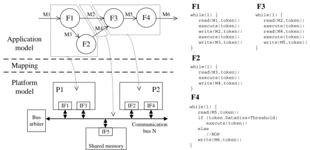
Following the Y-chart modeling approach [9], a system model is formed by a combination of an application model and a platform model. In the early design phase, full description of application functionalities is not mandatory and work-load models of the application are considered. A workwork-load model expresses the computation and communication loads that an application causes when executed on platform re-sources. An application workload model is structured as a network of concurrent communicating processes. Processes use abstract primitives to model communication and data processing (e.g., read, write, execute). Different communi-cation policies can be implemented to describe the way data are transferred and the dependencies between processes (e.g., rendezvous policy, FIFO policy with finite or infinite capac-ity). Fig. 1 depicts a didactic example of a system model. In this example, processes F1 and F2 are allocated to proces-sor P1 and processes F3 and F4 are allocated to procesproces-sor P2. The platform model could also include dedicated hard-ware resources to support process execution. The behaviour of each process is given in the right part of Fig. 1. In Fig. 1, relation M2 is communicated through shared communi-cation bus N by interfaces IF1 and IF2. Relation M4 is com-municated through shared communication bus N by inter-faces IF3 and IF4. The interinter-faces temporarily store data and manage transfers through the communication bus. A shared
F1 F3 F2 M1 M2 M4 M3 M5 Application model Platform model P1 P2 Communication bus N while(1) { read(M2,token); execute(token); read(M4,token); execute(token); write(M5,token); } while(1) { read(M1,token); execute(token); write(M2,token); execute(token); write(M3,token); } Mapping F4 F1 F2 F3 while(1) { read(M3,token); execute(token); write(M4,token); } M6 F4 while(1) { read(M5,token); if (token.DataSize>Threshold) execute(token); else //NOP write(M6,token); }
IF1 IF3 IF2 IF4
Shared memory Bus
arbiter
IF5
Fig. 1 Example of a system model based on three views: application, platform, and mapping.
memory is also shown. Schedulers are not illustrated in Fig. 1 since in the following we will focus on data flow oriented applications, with non-preemptive static order scheduling.
Academic system-level design approaches such as SCE [10], Sesame [11], SystemCoDesigner [17], and the ones presented in [1] and [19] were proposed to support the cre-ation process of performance models of hardware-software architectures. Industrial frameworks such as Intel CoFlu-ent Studio [15], Space Codesign [33], and Visualsim from Mirabilis Design [25] can also be cited.
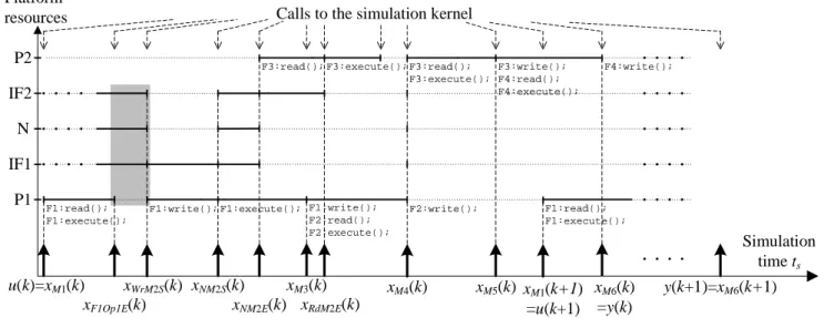
In the existing approaches, captured workload models are generated as executable descriptions and then simulated. Different approaches can be considered to generate and sim-ulate system models. In the trace-driven simulation approach [23], a platform model is driven by the traces caused by the application model execution. A trace represents the work-load imposed by a communication or a data processing prim-itive of the application on a platform element. A trace con-tains information on the communication and computation operations performed by the application process (e.g., size of communicated data). The execution time of each load primitive is approximated as a delay and the values of these delays are variable and data-dependent. Delays are com-monly expressed by analytical formulas and typically esti-mated from measurements on real prototypes or analysis of low level simulations, as illustrated in [19, 26]. The evolu-tion of a system model is thus a result of processing the computation and communication loads by the platform re-sources. During simulation, the simulation kernel schedules the execution of processes and manages the advancement of the simulation time. Simulation events occur at specific in-stants when processes synchronize between each other. Fig. 2 illustrates some of the events observed during simulation
of the example depicted in Fig. 11. In the considered
ple, delays can be variable and data dependent. As for exam-ple, in Fig. 2 the execution time of the execute statement of F1 is variable. In Fig. 2, instants xi(k) denote the
interme-diate synchronization instants involved in the system model execution. As for example, xW rM2S(k) denotes the k-th
in-stant at which a write operation starts at interface IF1. The instants related to communication through relation M2 are detailed in Fig. 2. For clarity reasons, the instants related to relations M1, M3, M4, M5, and M6 are not detailed. In the following, we denote the instant when an event occurs in the input of the system model by u and the instant when an event occurs in the output of the system model by y. In Fig. 2, u(k) denotes the k-th instant at which F1 receives a mes-sage through relation M1 and y(k) denotes the k-th instant at which F4 produces a message through relation M6.
Simulation of system models allows the influence of plat-form shared resources on application execution to be ana-lyzed. Concurrent accesses at shared resources lead to con-tentions, and thus additional delays are caused during sim-ulation of the system model. As an illustration of this phe-nomenon, let us consider that the platform interfaces cannot simultaneously be used for read/write operations and data transfer. In Fig. 2, the rectangle in grey highlights the situ-ation when IF1 is used for data transfer and the write oper-ation is delayed. Contention at shared resources can signif-icantly impact the execution of an application and therefore it must be thoroughly investigated in the system model sim-ulation. As this requires more time-consuming calls to the simulation kernel the overall simulation speed can be sub-stantially decreased.
1 In Fig. 2 and in the following of the article, the term ”simulation
Simulation time ts u(k)=xM1(k) xM1(k+1) =u(k+1) xWrM2S(k) xM3(k) F1:read(); F1:execute(); P1 Platform resources xM4(k) xM5(k) xM6(k) =y(k) y(k+1)=xM6(k+1) Calls to the simulation kernel
xNM2S(k) xNM2E(k) xRdM2E(k) F2:write(); F1:execute(); F1:write(); F2:read(); F2:execute(); P2 N F1:write(); F1:read(); F1:execute(); F3:read(); F3:execute(); F3:read();
F3:execute(); F3:write(); F4:read(); F4:execute(); F4:write(); xF1Op1E(k) IF1 IF2
Fig. 2 Discrete-event simulation of the system model with calls to the simulation kernel.
2.2 Improvement of simulation efficiency
Various approaches have been proposed to limit the number of simulation events while maintaining acceptable accuracy of system models.
The SystemC TLM2.0 standard [14] defines two coding styles to allow timing behaviour of architectures to be mod-eled at different abstraction levels: the approximately-timed coding style (TLM-AT) and the loosely-timed coding style (TLM-LT). Following the TLM-AT coding style, processes of the system model are annotated with specific delay values used in calls to the wait function. This coding style leads to a lock-step simulation that provides good accuracy but it causes excessive task switching overheads. To overcome this issue, the TLM-LT coding style supports the temporal decoupling method that allows processes to run ahead in a local time with no use of the simulator. The definition of a global quantum is thus needed to impose an upper limit on the time a process is allowed to run ahead of simulation time. However, this method leads to degraded timing accuracy be-cause delays due to access conflicts at shared resources are not simulated. The approach presented in this paper can be considered as intermediate between these two coding styles. Compared to the TLM-AT coding style, the number of calls to the simulator is decreased by grouping some of the pro-cesses of the system model and by computing during sim-ulation the values of delays. Similarly to TLM-LT, the pre-sented approach allows the number of events managed by the simulation kernel to be reduced. A simulation technique is introduced in this paper to consider delays due to potential access conflicts at shared resources.
Bobrek et al. [4] present a hybrid approach that com-bines discrete-event simulation with analytical models. It
aims at decreasing the simulation time of multi-processor platforms with minimum impact on accuracy compared to cycle-accurate models. The application processes are simu-lated for a period of time by ignoring contention at shared resources. An analytical model is then used to assign time penalties to the competing processes that access to shared resources. The time penalties shift the execution time of the processes running on shared resources. A similar approach is presented by Chen et al. in [7]. It details an analytical model that gives the contention delay under different multi-processor platform configurations and bus utilization rates. This analytical model is used during simulation of the bus model and it prevents full scheduling of events. Compared to these two approaches, our method aims to greatly reduce the number of context switches among processes managed by the simulation kernel.
In [28], Savoiu et al. present an approach to improve simulation performance of SystemC models. This approach consists in restructuring SystemC models to limit the num-ber of calls to the simulator. SystemC models are first con-verted into Petri nets to be analyzed. Reduction methods are then applied to create an equivalent Petri net but with a lim-ited number of cycles. Finally, an improved SystemC model is obtained from the reduced Petri net. In our approach, we also consider Petri nets as an intermediate representation for workload models. We use this intermediate representation to compute the synchronization instants among the elements of the system model with no use of the simulator. However, we do not consider here the possible reduction of the obtained Petri nets.
In [20], K¨unzli et al. present a hybrid approach to im-prove performance evaluation of data flow oriented systems. The presented approach combines analytical models of
sys-tem components and simulation to achieve good compro-mise between simulation speed and accuracy. Analytical mod-els are based on the real-time calculus (RTC) formalism pre-sented in [6]. This formalism is based on the concept of ar-rival curves and service curves that respectively characterise workload and processing capabilities of system components. For a given event stream, arrival curves express lower and upper bounds on the number of events arriving in any time interval. In [20], simulation traces are analyzed to determine arrival curves. The curves are then passed to the formal anal-ysis method and the results from the analanal-ysis method are transformed into event traces used for simulation. Compared to a simulation model, execution of hybrid models is signif-icantly sped-up because the number of calls to the simulator is limited. Our proposed approach can also be considered as a hybrid approach that combines simulation and formal models. In contrast to [20], our approach does not focus on prediction of best and worst cases.
The result-oriented modeling (ROM) approach has been proposed by Schirner and D¨omer in [29, 30] to improve the simulation speed-accuracy tradeoff in discrete-event mod-els of communication resources and operating systems. The principle of this approach is to optimistically predict the stants when modeled elements evolve, using available in-formation about resources. The estimated instants are then adapted during simulation in the case of disturbing influ-ences such as pre-emption of shared resources. In our pro-posed approach, the simulation instants are not estimated but computed during simulation. Compared to ROM, this ap-proach allows more events to be saved and potentially better simulation efficiency.
In [18], simulation constructs are proposed to support creation of accuracy adaptive transaction level models. The created models incorporate multiple levels of timing accu-racy and levels can be changed statically at the start of sim-ulation or at runtime. Our proposed approach also considers a reduced number of timing annotations but with no degra-dation of timing accuracy.
In [34] and [24], simulation techniques are presented that address the timing accuracy problem in temporally de-coupled transaction level models. In [34], a central instance keeps track of all transactions that are potentially influenced by other processes and that have not yet synchronized their local time. Once a synchronization point is reached, conflict-ing transactions are arbitrated and execution times can be re-vised with a posteriori knowledge. In [24], an analytical tim-ing estimation method is proposed. Accordtim-ing to the consid-ered arbitration policy of shared resources, some analytical expressions are defined that give time penalties. Resource usage and resource availability are used to derive the delay formulas. These formulas are then used during simulation to correct the end of each synchronization request. In the same way as in [34, 24], our approach performs retroactive timing
correction but does not consider TLM-LT models. Besides, we use knowledge about application and platform to reduce the required calls to the simulation kernel.
Razaghi and Gerstlauer present in [27] a conservative simulation approach for multi-core operating system model called automatic timing granularity adjustment (ATGA). ATGA is used to control the advancement of the simulation time and to invoke the simulation kernel whenever a task pre-emption is required. In predictive mode, the state of running periodic tasks is monitored to determine instants when pre-emption occurs among tasks. A fallback mode is also imple-mented that enables asynchronously interrupting long time periods. In our approach, the advancement of the simulation time is done according to computations performed during simulation. Adaptation of the computed instants is required in the case of conflicting accesses at shared resources.
The main thrust of the proposed simulation approach is to reduce the number of required calls to the simulation ker-nel and to keep accurate the influence of shared resources. The idea of instantaneous computation of synchronization instants was first presented and evaluated in [22] but we did not present how computation could be performed systemat-ically. Besides, the necessity to correct computed instants in the case of shared resources was not considered in [22]. We introduced the idea of correction of synchronization instants in the case of shared resources in [21] but with no details about the implementation of this method. In this article, we present more details of our existing work with the following contributions:
– We present the adoption of the timed Petri net formalism for both the computation and correction of synchroniza-tion instants. This formalism is adopted to better justify the feasibility of the computation and correction meth-ods. Some Petri net patterns are introduced to capture the time dependencies among elements of a system model. – We detail the implementation of the proposed hybrid
simulation approach, combining formal and simulation models.
– Based on the timed Petri net formalism, we present the implementation of the correction technique and evalua-tion of the scalability of this technique.
– We illustrate application of the proposed simulation ap-proach through a case study inspired from communica-tion systems.
3 Principles of the proposed simulation approach Compared to the existing simulation approaches, the pro-posed simulation approach uses knowledge about applica-tion and platform to limit the number of required calls to the simulation kernel. We consider that some parts of a sys-tem model can be abstracted and replaced by an
equiva-lent executable model. This executable model presents the same evolution as the abstracted elements from an exter-nal viewpoint, but the number of events managed by the simulation kernel is reduced. The equivalent model incorpo-rates the expressions of the synchronization instants among the abstracted elements2. In section 4, we adopt the timed
Petri net formalism to express the time dependencies among the abstracted elements and the related synchronization in-stants. This formal representation is used to compute the synchronization instants during simulation and to determine the execution order between the abstracted processes. This approach allows data-dependent behaviors to be considered (e.g., behavior with delays that depend on exchanged data, behavior with condition on production or reception of data). Data dependencies can be formulated through the created timed Petri net and influence execution of the equivalent ex-ecutable model. The key point of our approach is that the synchronization instants are instantaneously computed dur-ing simulation, i.e. with no involvement of the simulation kernel.
Fig. 3 illustrates the idea of instantaneous computation in comparison with the execution depicted in Fig. 2. In Fig. 3, instants y(k) and y(k + 1) are respectively computed at instants u(k) and u(k + 1). The computation of intermedi-ate synchronization instants xiand synchronization instant y
at the output of the executable model is denoted by action Compute_y(). Compared to the execution depicted in Fig. 2, intermediate synchronization instants xiare locally
com-puted and stored but no intermediate event is caused during the model execution. The simulation is thus faster because the number of calls to the simulation kernel is reduced, while timing accuracy is preserved. Time dependencies among the synchronization instants can be formulated by the following state equations:
X(k) = f (X (k), X (k − 1), . . . , X (k − a), u(k), . . . , u(k − b)) (1) y(k) = g(X (k), . . . , X (k − c), u(k), . . . , u(k − d)) (2) X(k) denotes the set of intermediate synchronization instants xi(k) among the abstracted elements. f reflects the
depen-dencies between current intermediate instants X (k), previ-ous intermediate instants, and synchronization instants at the input of the system model. g reflects the dependencies between current synchronization instants y(k) at the out-put of the system model, intermediate synchronization in-stants, and synchronization instants at the input of the sys-tem model. For illustration purposes and with no loss of gen-erality, we will only discuss models with one input and one output. In the following, state equations (1) and (2) will be expressed through a timed Petri net.
2 Besides, application functionalities can be incorporated into the
proposed equivalent model.
The presented approach reduces the number of events managed by the simulation kernel. In the case of shared re-sources, a disturbing influence3can cause the computed
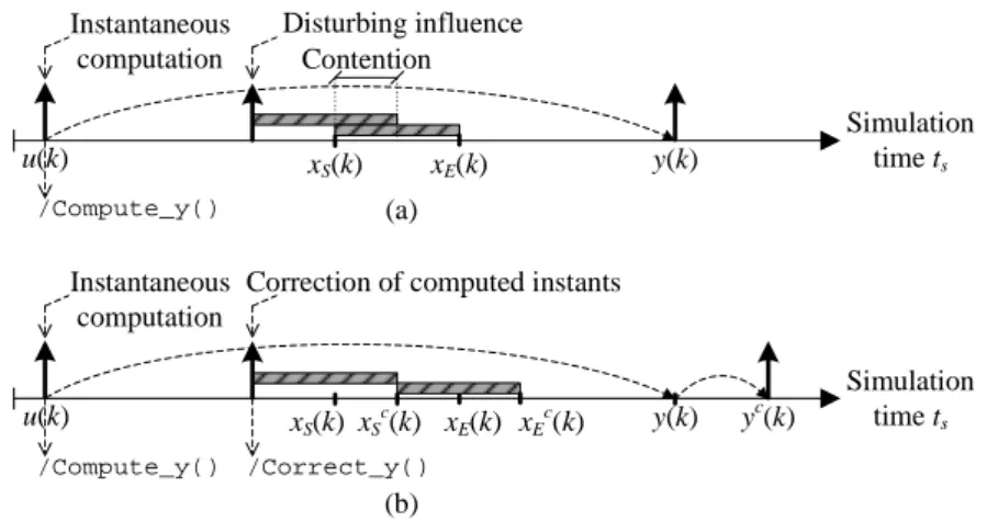
syn-chronization instants to become inaccurate because delays due to access conflicts at shared resources are not simulated. We propose to utilize the expression of synchronization in-stants to detect potential conflicts at shared resources and to correct the erroneous computed instants. This idea is illus-trated in Fig. 4, where the shaded rectangles correspond to the intervals of time when a shared resource is used. xS(k)
and xE(k) correspond to the instants when the usage of the
shared resource starts and ends4. Instants x
S(k), xE(k), and
y(k) are computed at instant u(k) using the approach illus-trated in Fig. 3. In part (a) of Fig. 4, a disturbing influence occurs before xS(k) and it causes usage of the shared
re-source. In the case of a shared resource for which simulta-neous usage is not possible (i.e. with limited concurrency), computed instants xS(k), xE(k), and y(k) become incorrect.
Application of the proposed correction technique is shown in part (b) of Fig. 4. The key idea of the correction technique is to re-evaluate state equations (1) and (2) when the dis-turbing influence occurs. We recall that these equations cap-ture the influence of shared resources and the related delays. The disturbing influence is taken into account straight and it modifies some of the intermediate instants. The state equa-tions are thus re-evaluated with new initial values and in-ternal state X (k) is adjusted accordingly. Output simulation instant y(k) is also corrected. The correction is performed instantaneously with no involvement of the simulation ker-nel. This correction is denoted in part (b) of Fig. 4 by action Correct_y(). In the situation depicted in part (b) of Fig. 4, xS(k) is corrected and set to the instant when the resource is
available. This corrected instant is denoted by xcS(k). Based on this corrected value, previously computed instants xE(k)
and y(k) are recalculated through equations (1) and (2), re-sulting in xcE(k) and yc(k). With this technique, the delays due to contention at shared resources are inserted with no in-volvement of the simulation kernel. Accurate evaluation can thus be achieved with a reduced set of events. In the scope of this paper, we will illustrate the application of this ap-proach for shared communication resources. Similarly, con-tention at computation and memory resources could also be addressed.
The presented simulation approach combines thus in-stantaneous computation and correction of synchronization instants. We successively detail these two techniques in the following of this paper.
3 Disturbing influence designates any simulation event that causes
contention at a shared resource.
4 As an example, in Fig. 2 interface IF1 is used for data exchange
through communication bus N. xS(k) could represent the k-th instant
/Compute_y() /Compute_y()
Simulation time ts
u(k) u(k+1) y(k) y(k+1)
Instantaneous computations
Fig. 3 Proposed hybrid simulation approach with instantaneous computation of synchronization instants.
/Compute_y() Simulation time ts u(k) Disturbing influence y(k) xS(k) xE(k) /Compute_y() Simulation time ts u(k) xS(k)xSc xE(k) y(k) (k) xEc(k) /Correct_y() yc(k) (a) (b) Contention
Correction of computed instants Instantaneous
computation
Instantaneous computation
Fig. 4 (a) Simulation with erroneous computed instants in the case of a shared resource, (b) simulation with correction of computed instants.
4 Computation of synchronization instants
We describe the technique for computing synchronization instants. The timed Petri net formalism is adopted to formu-late the synchronization instants among the abstracted el-ements of the system model. We first give some basic cepts related to timed Petri nets. Second, we present the con-struction of timed Petri nets from system models. Third, we explain the way expression of synchronization instants and executable models are combined.
4.1 Timed Petri nets
Petri nets represent a powerful modeling language that is well adapted for formal description of discrete-event sys-tems. Timed Petri nets represent a timed extension of Petri nets for which time is expressed as minimal durations on the sojourn of tokens in places [2]. A timed Petri net is defined as a tupleT = (P,Q,•(.), (.)•, µ0, T, ρ) where:
– P = p1, . . . , pmis a finite, non-empty set of places,
– Q = q1, . . . , qnis a finite, non-empty set of transitions,
– •(.) ∈ (N|P|)|Q|is the backward incidence function, – (.)•∈ (N|P|)|Q|is the forward incidence function, – µ0∈ N|P|is the initial marking of the net,
– T ∈ R|P|is the set of holding times of places,
– ρ ∈ N|P| is the set of switching sequences attached to places.
Each transition q is characterised by its backward and for-ward incidence functions. They indicate the weight of each
arc that connects a place and a transition. A marking µ of the net is an element of N|P| such that µ(p) is the num-ber of tokens in place p. Each place has an infinite capacity. Basically, a transition q is enabled if each upstream place contains at least one token. A firing of an enabled transition removes one token from each place of its upstream places and adds one token to each of its downstream places. In a more general way, weights are attached to arcs. A transi-tion is thus enabled if the upstream places contain at least the number of tokens given by the weight of the connecting arcs. Similarly, after the firing of a transition, a downstream place receives the number of tokens given by the weight of the connecting arc. In the following, when not indicated, the weight of the arc is equal to 1. The holding time of a place is the time a token must spend in the place before contribut-ing to the enablcontribut-ing of the downstream transitions. Holdcontribut-ing times can depend on the index of the firing. Each place p that has several downstream transitions receives a switching sequence ρ(p). It defines the transition to which the token must be routed. Only tokens such that ρ(p) = q should be taken into account by q. Fig. 5 illustrates a simple timed Petri net with seven places and six transitions. In the situa-tion depicted in Fig. 5, tokens are initially set into places p4
and p6.
We denote xj(k) j = 1, . . . , |Q|,k ≥ 0, as the instant when
transition qj is enabled for the k-th time. Relationships
be-tween transition instants can basically be expressed using two operators: addition and maximization. Addition expresses a time lag according to an holding time. Maximization
re-q2 p3 q3 q4 p4 Tp5 q5 p5 q1 q0 p0 p1 p2 Tp3 Tp1 Tp2 Tp0 p6
Fig. 5 Example of a timed Petri net with seven places and six transi-tions.
flects the effect of synchronization. With the initial marking depicted in Fig. 5, the transition instants are given as fol-lows: x1(k) = max(Tp0(k) + x0(k), x2(k − 1)) x2(k) = Tp1(k) + x1(k) x3(k) = Tp2(k) + x1(k) x4(k) = max(Tp3(k) + x2(k), x3(k − 1)) x5(k) = Tp5(k) + x4(k)
Considering X (k) as the vector formed by transition instants xj(k) of the timed Petri net, the transition instants can be
ex-pressed through state equations similar to (1) and (2). The state equations are obtained by considering input transition instant u(k) as x0(k) and output transition instant y(k) as
x5(k)5. Extensive presentation of the theoretical framework
that justifies and analyzes such state equations for timed Petri nets can be found in [2]. In the scope of this paper, we adopt the state equation notation to conveniently explain the developed simulation techniques.
4.2 Construction of a timed Petri net
The timed Petri net notation is adopted here to formulate the time dependencies among the elements of a system model and the related synchronization instants. A timed Petri net is constructed by successively considering the application description, the mapping, and the platform constraints. El-ementary timed Petri net patterns must be defined for each statement of the system model. The timed Petri net related to the system model is then obtained by connecting the patterns together. First, connection between patterns is done con-sidering the behavioral description of each process and the structural description of the application. Second, the timed Petri net associated with the system model is formed con-sidering the mapping and platform constraints. A similar ap-proach was adopted in [32] considering the enhanced func-tion flow block diagram (EFFBD) notafunc-tion. In this paper, we
5 In this simple example, we obtain state equations with a = 1, b =
c= d = 0. Besides, y(k) does not depend on u(k) in equation (2).
q(Op)p(Op)q(/Op) p0(Op)
TOp
Fig. 6 Petri net pattern of the computation statement.
do not use a specific notation for the system model and we give patterns for some elementary modeling statements.
As previously illustrated, application workload models are made of three categories of modeling statements:
– the computation statement (e.g., execute) models the data processing in application processes,
– the communication statements (e.g., read, write) model the communication protocols among processes of the ap-plication,
– the control statements (e.g., alternative, iteration) describe the control flow of each elementary process of the appli-cation.
We associate a Petri net pattern with each statement of the application model. Each pattern n can formally be defined by a Petri netTn. The Petri net related to an application
model is obtained by connecting each elementary pattern n. The timed Petri net associated with the system description is then formed by considering the mapping and the platform constraints. First, delays due to execution of application on platform resources are taken into account. Holding times are added to places of the Petri net to represent computation and communication delays. Second, the limited concurrency of platform resources is considered by adding supplementary places and arcs to the created Petri net. These places and arcs cause additional conditions to enable Petri net transitions. In the following, we present patterns with time constraints. These patterns correspond thus to elements of the applica-tion model that are allocated to computaapplica-tion or communica-tion resources. Each pattern begins with an entry place and ends with a transition. Dashed lines represent possible con-nections with other patterns.
The pattern associated with the computation statement is represented in Fig. 6. Transitions q(Op) and q(Op) denote the instants at which the computation starts and ends. Place p(Op) denotes the execution of the computation whereas p0(Op) represents the condition before the beginning of the
computation. Duration TOp represents the execution time of
the operation for the considered computation resource. TOp
can be variable and data dependent and it can be expressed by an analytical formula.
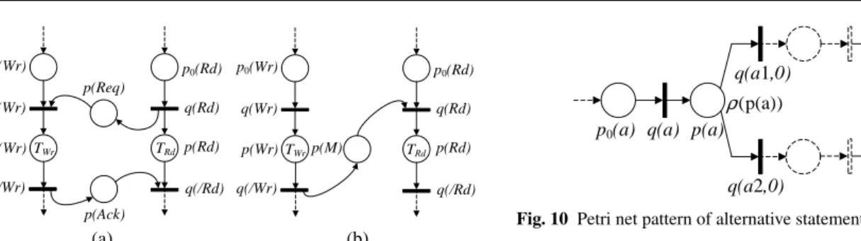
According to the communication protocol between pro-cesses of the application, different patterns can be associated with the communication statements. Part (a) of Fig. 7 illus-trates the pattern for the rendezvous communication proto-col. Transition q(Rd) represents the instant when the writer
(a) (b) q(Rd) q(/Rd) p(M) p(Rd) q(Wr) q(/Wr) p(Wr) p0(Wr) p0(Rd) q(Rd) q(/Rd) p(Ack) p(Rd) q(Wr) q(/Wr) p(Wr) p0(Wr) p0(Rd) p(Req) TWr TRd TWr TRd
Fig. 7 Petri net pattern of the communication statements: (a) ren-dezvous protocol, (b) FIFO protocol with infinite capacity.
q(i,0) q(/i) p0(i) inf q(i) p(i) p(i,0) p(/i) Fig. 8 Petri net pattern of the infinite loop statement.
q(f,0) q(/f) p0(f) N q(f) p(f) p(f,0) p(/f) p(le) q(le) N
Fig. 9 Petri net pattern of the finite loop statement.
and the reader are synchronized and the data transfer is done. Part (b) of Fig. 7 illustrates the pattern for the FIFO protocol with infinite capacity. Transitions q(W r) and q(Rd) denote the instants at which write and read operations start. TW rand
TRd represent the duration of write and read operations for
the considered computation resource. They can also be vari-able and data dependent and they can be expressed by an analytical formula.
The infinite iteration statement is depicted in Fig. 8. Tran-sitions q(i, 0) and q(i) denote the instants when one iteration starts and ends. Place p(i, 0) is needed because only one it-eration can take place at the same time. Symbol in f means that an infinite number of tokens is added to place p(i) when q(i) is enabled.
The pattern associated with the finite iteration statement is represented in Fig. 9. Symbol N represents the number of iterations of the loop. Transition q(le) denotes the instant when N iterations of the loop have been performed. Place p( f , 0) indicates that only one iteration can take place at the same time.
The alternative statement indicates which set of instruc-tions is executed, according to condiinstruc-tions. The pattern asso-ciated with the alternative statement is represented in Fig. 10. The switching sequence ρ(p(a)) indicates the selection between transitions q(a1, 0) and q(a2, 0) when a token is into place p(a).
q(a1,0)
q(/a) p0(a) q(a) p(a) p(/a)
q(a2,0)
(p(a))
ρ
Fig. 10 Petri net pattern of alternative statement.
We illustrate now the modeling of a shared resource with limited concurrency. We consider here the situation where communication between processes is done through two in-terfaces and a communication bus. As in the example of Fig. 1, we assume that data transfers and read/write operations cannot be performed simultaneously. Fig. 11 illustrates the pattern in the case of a direct data transfer with no usage of a shared memory. The considered bus arbitration policy corresponds to a First Come First Serve (FCFS) policy but other arbitration policies could be modeled. TW rrepresents
the duration of the write operation into the interface, TRd
rep-resents the duration of the read operation from the interface. TN represents the transfer duration through communication
bus N. Places p(IF1) and p(IF2) model the limited concur-rency of interfaces IF1 and IF2. In Fig. 11, once transition q(W r) is enabled, tokens that are stored in p(M) cannot be processed until q(W r) is enabled. A similar pattern could be built in the case of a computation resource with limited concurrency.
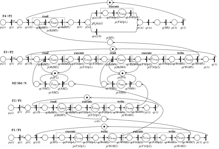
The presented patterns are used to create a timed Petri net in association with the elements of a system model. As an illustration, Fig. 12 represents the timed Petri net related to the example depicted in Fig. 1. The depicted Petri net is obtained by connecting together the patterns related to the communication, computation, and control statements. In Fig. 12, the FIFO communication protocol with infinite ca-pacity is considered. The communications through relations M2, M3, M4, and M5 are detailed. TNM2and TNM4represent
the transfer durations through communication bus N. In Fig. 12, all the considered delays can be variable and data de-pendent. Places p(IF2) and p(IF4) express that data trans-fer and read operation cannot be performed simultaneously by interfaces IF2 and IF4. Places p(IF1) and p(IF3) and related arcs are not depicted in Fig. 12 for clarity reasons. In Fig. 12, a switching sequence, denoted by ρ(p(a)), is attached to place p(a). It models the alternative statement used in process F4 of Fig. 1. The created timed Petri net highlights the time dependencies among the elements of the system model and the related synchronization instants. Es-pecially, it gives the time dependencies between the transi-tion instants that are related to the input and the output of the system model (i.e. transitions q(M1) and q(M6) in Fig. 12).
TRd read q(Rd) p(Rd) q(/Rd) p0(Rd) data transfer q(N) p(N) q(/N) TN write q(Wr) p(Wr) TWr q(/Wr) p(IF2) p(IF1) p(M) p0(Wr)
Fig. 11 Petri net pattern in the case of a communication through two interfaces and a communication bus.
F1 / P1 inf TF1Op1 TF1Op2 F4 / P2 inf TF4Op1 TWrM2 TWrM3 TRdM5
execute write execute write
read
execute
p0(i) q(i) p(i) q(i,0) q(M1)
p(F1Op1) q(F1Op1) q(/F1Op1) q(WrM2) p(WrM2) q(/WrM2) q(F1Op2) q(/F1Op2) p(F1Op2) q(WrM3) p(WrM3) q(/WrM3)p(/i)q(/i) p(M3)
p0(i) q(i) p(i) q(i,0) q(RdM5)
p(RdM5) q(/RdM5) q(F4Op1) p(F4Op1) q(/F4Op1) p(/i) q(/i) p(M5) p(a) p(/a) q(M6) q(a) q(a1,0) q(a2,0) q(/a) inf TF2Op1 TRdM3 TWrM4
read execute write
p0(i) q(i) p(i) q(i,0)
p(RdM3) q(RdM3) q(/RdM3) p(F2Op1) q(F2Op1) q(/F2Op1) q(WrM4) p(WrM4) q(/WrM4)p(/i) q(/i) inf TF3Op1 TF3Op2 TRdM2 TRdM4 TWrM5
read execute read execute write
p0(i) q(i) p(i) q(i,0)
p(RdM2) q(RdM2) q(/RdM2) p(F3Op1) q(F3Op1) q(/F3Op1) q(RdM4) p(RdM4)q(/RdM4) q(F3Op2) q(/F3Op2) p(F3Op2) q(WrM5) p(WrM5) q(/WrM5) q(/i) p(/i) F2 / P1 F3 / P2 TNM2 TNM4 q(NM4) q(/NM4) M2 M4 / N q(NM2) q(/NM2) p(NM2) p(NM4) p(IF2) p(IF4) )) ( (pa ρ
Fig. 12 Timed Petri net associated with the architecture model depicted in Fig. 1.
We use this formal model to compute the synchronization instants among the elements of the system model.
4.3 Combination between formal and executable models The dependencies among transition instants can be practi-cally captured through a directed graph, that we call a tem-poral dependency graph. A temtem-poral dependency graph ex-presses the dependencies among the transition instants of the created timed Petri net. It can also be seen as a convenient way to express the evolution of X (k) and y(k) and to imple-ment state equations (1) and (2). The nodes of a temporal
dependency graph correspond to the transition instants of the created timed Petri net. The arcs give the dependencies among the transition instants. The weights associated with the arcs correspond to the delays between the transition in-stants. In the following, storage of the computed transition instants is done through a one dimensional array denoted by G, which size is denoted by kG. G aims to temporarily store the set of intermediate instants that are involved in the computation of synchronization instants X (k) and y(k). As an illustration, Fig. 13 depicts a part of the temporal depen-dency graph related to the timed Petri net of Fig. 12 and the related array G. In this example, the complete temporal
de-pendency graph contains 46 nodes. The transition instants are successively computed by traversing a temporal depen-dency graph. Traversing of the temporal dependepen-dency graph is performed in accordance with the created timed Petri net. Some of the computations performed when traversing the temporal dependency graph depicted in Fig. 13 are given below:
u(k) = max(xM1(k), xM3W rE(k − 1));
xF1Op1S(k) = xM1(k);
xF1Op1E(k) = xF1Op1S(k) + TF1Op1(k));
xaS(k) = xM5RdE(k);
if (token.DataSize > Threshold){ xa1(k) = xaS(k);
xF4Op1S(k) = xa1(k);
xF4Op1E(k) = xF4Op1S(k) + TF4Op1S(k);
xaE(k) = xF4Op1E(k); } else{ xa2(k) = xaS(k); xaE(k) = xa2(k); } y(k) = xM6(k) = xaE(k);
In the proposed approach, the system model is simulated through an executable model that presents the same evolu-tion as the abstracted processes from the external viewpoint. This executable model uses the synchronization instants at the input of the system model to compute the intermediate synchronization instants and the synchronization instants at the output of the system model. The computation uses the constructed temporal dependency graph and related array G. The evolution of the executable model mainly depends on two categories of time interval:
– the minimal interval of time before an output is pro-duced, denoted by Ty,
– the minimal interval of time before an input can be con-sumed, denoted by Tu.
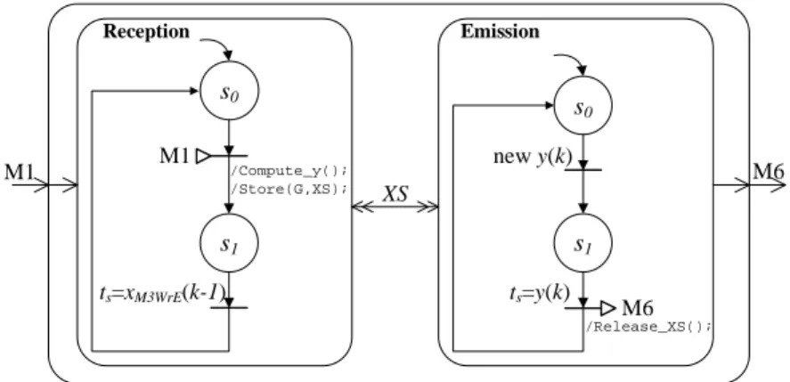
Fig. 14 gives the structural and behavioural description of the executable model for the example of Fig. 1. Two cesses are handled by the simulation kernel. The input pro-cess, denoted by Reception, receives input data and com-putes the synchronization instants through action Compute_y(). This action uses array G to locally compute and store the synchronization instants. The computed synchronization in-stants are then copied in a variable denoted by X S. X S is a two dimensional array that temporarily stores the computed synchronization instants that have not yet been achieved dur-ing simulation. The dimensions of array X S have ranges 0 to
kG− 1, and 0 to kS− 1. kSsets of synchronization instants
can thus be stored in data structure X S. The ouput process, denoted by Emission, is activated each time a new output instant has been computed. The k-th output data is produced at instant y(k). In Fig. 14, the k-th input data can be received when instant xM3W rE(k − 1) is achieved. Intervals of time Tu
and Ty correspond to the duration of state s1in processes
Reception and Emission. The k-th set of synchronization in-stants stored in X S is released when y(k) is achieved. This is denoted by action Release_XS() in Fig. 14. The exe-cutable model depicted in Fig. 14 can be adopted for system models with one input and one output. It can be extended to consider multiple inputs and multiple outputs.
The upper part of Fig. 15 illustrates the execution of the equivalent model over the simulation time. When a new data is received through relation M1 at instant xM1(k), the value
of output evolution instant xM6(k) is instantaneously
com-puted and stored. Intervals of time Tuand Tyare determined
through action Compute_y(). The evolution over the simu-lation time of the equivalent executable model only depends on computed values Ty and Tu. The intermediate
synchro-nization instants are also computed at instant xM1(k). The
lower part of Fig. 15 represents the computed intermediate synchronization instants. This observation is performed us-ing a local time called observation time, denoted by to. The
evolution of the resource usage between xM1(k) and xM6(k)
is done without using the simulator. In Fig. 15, the correc-tion technique is not yet considered.
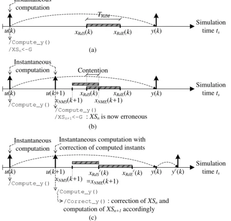
5 Correction of computed synchronization instants The presented computation technique allows the number of events managed by the simulation kernel to be reduced. How-ever, the computed synchronization instants potentially need to be updated to correctly reflect the influence of shared re-sources. Fig. 16 illustrates such a potential issue. It focuses on the situation when a communication node and an inter-face are used for data transfer. In part (a) of Fig. 16, instants xRdS and xRdE correspond to the instants when an interface
read operation starts and ends. The shaded rectangle rep-resents the interval of time when the interface is used for reading. Instants xRdS(k), xRdE(k), and y(k) are computed
at instant u(k) using the previously presented approach. In part (b) of Fig. 16, the instants at which a new data trans-fer starts and ends are computed at instant u(k + 1). They are denoted by xNMS(k + 1) and xNME(k + 1). In this
situ-ation, the interface is thus simultaneously used to transfer data through node N and to provide the previously received data. In the case of an interface with limited concurrency, these two operations cannot be performed simultaneously and the computed instants are erroneous. The application of the proposed correction technique is illustrated in part (c) of Fig. 16. Once computed, instants xNMS(k + 1) and
0 TF1Op1(k) xF1Op1S(k) xF1Op1E(k) xM2WrS(k) 0 xM1(k) xM2WrE(k) xM5RdE(k) xF4Op1S(k) xaE(k) xa2(k) 0 TWrM2(k) TRdM5(k) xa1(k) TF4Op1(k) 0 0 0 0 0 xM6(k-1) xM3WrE(k-1) xaS(k) 0 xM6(k)=y(k) xF4Op1E(k) 0 0 xM5RdS(k) G=[xM1(k), xF1Op1S(k), xF1Op1E(k), xM2WrS(k), …, xM6(k-1), xM6(k)], kG=46
Fig. 13 Temporal dependency graph used to compute transition instants.
s0 M1 /Compute_y(); /Store(G,XS); Reception Emission s0 s1 M6 M1 M6 XS ts=y(k) new y(k) s1 ts=xM3WrE(k-1) /Release_XS();
Fig. 14 Structural and behavioural description of the equivalent executable model.
u(k)=xM1(k) u(k+1)=xM1(k+1) Simulation time ts (a) (b) Ty(k) Ty(k+1) /Compute_y() /Store(): XSn<-G /Compute_y() /Store(): XSn+1<-G y(k)=xM6(k) Tu(k) Tu(k+1) Observation time to TF3Op1(k) xM3WrE(k) /Release_XS(): XSn is released u(k)=xM1(k) xM1(k+1) =u(k+1) xWrM2S(k) xM3WrE(k) xWrM2S(k+1) P1 Platform resources xM4(k) xM5(k) xM6(k) =y(k) y(k+1)=xM6(k+1) xNM2S(k) xNM2E(k) xRdM2E(k) P2 N IF1 IF2
TF1Op1(k) TWrM2(k) TF1Op2(k) TF2Op1(k) TF1Op1(k+1)
TF3Op2(k) TF4Op1(k) TNM2(k) TWrM2(k) TRdM2(k) TRdM2(k) y(k+1)=xM6(k+1)
Fig. 15 Execution of the system model using instantaneous computation of evolution instants, evolution is over the simulation time (a) and the observation time (b).
xNME(k + 1) are compared to the previously computed
in-stants and a contention at the interface is detected. Instant xRdS(k) is thus corrected accordingly. The previously
com-puted instants that depend on xRdS(k) are then recomputed.
The recomputation is done using the expression of the syn-chronization instants. In Fig. 16, these operations are
de-noted by action Correct_y(). The corrected synchroniza-tion instants are denoted by xcRdS(k), xcRdE(k), and yc(k).
The correction technique is implemented in the equiva-lent executable model presented in Fig. 14. The correction technique is used during simulation to evaluate a new time the previously computed instants. This can be perceived as
/Compute_y()
Simulation time ts
u(k) xRdS(k) xRdE(k) y(k)
/Compute_y()
Simulation time ts
u(k) xRdSc(k) xRdEc(k) y(k)
/Correct_y() : correction of XSn and
computation of XSn+1 accordingly
yc(k) (b)
(c) Contention
Instantaneous computation with correction of computed instants Instantaneous computation Instantaneous computation /Compute_y() Simulation time ts
u(k) xRdS(k) xRdE(k) y(k)
(a) Instantaneous computation u(k+1) xNMS(k+1) xNME(k+1) u(k+1) xNMS(k+1) =x NME(k+1) TRdM /Compute_y() /Compute_y() /XSn<-G /XSn+1<-G : XSn is now erroneous
Fig. 16 (a) Equivalent model execution with usage of a shared resource, (b) disturbing influence in the case of a shared resource, (c) equivalent model execution with correction of computed instants.
computing state equations (1) and (2) with new intermediate instants. When a contention is detected, action Correct_y() adjusts the previously computed instants stored in data struc-ture X S. We explain here the use of data strucstruc-tures G and X S to correct the previously computed instants. As illustrated in Fig. 16, we consider here that n + 1 sets of synchronization instants are stored in X S when a correction occurs. We de-note by X Sm,nthe previously computed instant that must be
corrected. We denote by GSand GEthe newly computed
in-stants when usage of a shared resource starts and ends. The basic steps of the correction process are given as follows:
1. (Contention detection.) If GS< X Sm,n< GE, set X Sm,n←
GE.
2. (Temporary saving of data structure G.) For each syn-chronization instant i from 1 to p, set Di← Gi.
3. (Initialize data structure G.) For each synchronization in-stant i from 1 to p, set Gi← XSi,n.
4. (Recomputation of synchronization instants.) For each synchronization instant i from p + 1 to kG:
(a) Compute Gi.
(b) Set X Si,n← Gi.
5. (Recovery of data structure G.) For each synchronization instant i from 1 to p, set Gi← Di.
6. (Return data structure X S.) Return X Sn.
In step (1), when a contention is detected, previously com-puted instant X Sm,n is corrected and set to GE. In step (2),
the values stored in data structure G are temporarily saved because G is used for recomputation. In step (3), G is initial-ized with some of the previously computed instants. We de-note by p the number of synchronization instants that must be loaded in data structure G before recomputation. In step (4), the synchronization instants are successively recomputed and stored in data structure X S. Recomputation is still done by traversing the defined temporal dependency graph. Fi-nally, data structure G is recovered in step (5) to allow the computation of new intermediate synchronization instants. In that case, the complexity of the correction technique is related to the number of synchronization instants to be re-computed.
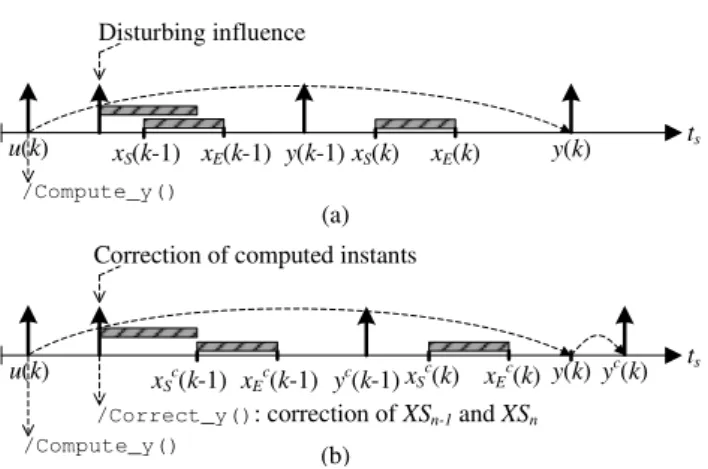
In the presented situation, only one set of synchroniza-tion instants stored in X S is modified. More generally, the correction of previously computed instants can concern var-ious sets of synchronization instants. This situation is illus-trated in Fig. 17. In the upper part of Fig. 17, a disturbing influence causes xS(k − 1), xE(k − 1), xS(k), and xE(k) to
become erroneous. The correction of the computed instants is considered in the lower part of Fig. 17. The correction can be perceived here as using state equations (1) and (2) to successively compute X (k − 1), y(k − 1), and then X (k),
/Compute_y() ts u(k) Disturbing influence y(k) xS(k) xE(k) /Compute_y() ts u(k) y(k)
/Correct_y(): correction of XSn-1 and XSn
yc(k)
(a)
(b) Correction of computed instants
xS(k-1) xE(k-1) y(k-1) xS c (k-1) xE c (k-1) yc(k-1) xS c (k) xE c (k)
Fig. 17 (a) Disturbing influence in the case of a shared resource, (b) equivalent model execution with correction of multiple sets of synchro-nization instants.
y(k). During the correction process, steps (3) and (4) must be performed iteratively to correct the required sets of synchro-nization instants stored in X S. Therefore, the complexity of the correction technique depends on the number of synchro-nization instants and the number of sets of synchrosynchro-nization instants to correct. The influence of the complexity of the correction technique is evaluated in next section.
6 Experiments
Validation of the proposed simulation approach is first pre-sented. We then estimate the influence of the complexity of the proposed approach. Finally, the benefits of the simula-tion approach are highlighted through a case study.
6.1 Validation of the simulation approach
Validation of the proposed simulation approach first con-cerns the Petri net patterns used for computation of synchro-nization instants. We considered the industrial modeling and simulation framework Intel CoFluent Studio [15] to capture system models and to compare achieved simulation results when using the proposed simulation approach. Using this framework, system models are typically described through three views: application, platform, and mapping views. Once captured, system models are generated as SystemC descrip-tions and then their execudescrip-tions can be analyzed. We estab-lished Petri net patterns for the main modeling statements supported by Intel CoFluent Studio. The equivalent model depicted in Fig. 14 was captured to allow simulation with the proposed approach. The implementation of actions Compute_y() and Correct_y() corresponded to C++ code developed to compute and correct synchronization instants. The Petri net patterns were validated by comparing the achieved simula-tion results for various system models. Models were simu-lated with randomly spaced input stimuli and random values
of delays for computation and communication statements. Models were run on a 2.80 GHz Intel-E5 machine with 8 GBytes RAM.
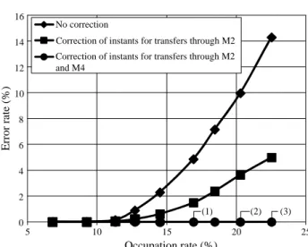
We consider here the didactic example of Fig. 1 to il-lustrate the benefits of the proposed approach. In this ex-ample, the communication interfaces are the only shared resources of the platform model with limited concurrency, i.e. read/write operations and data transfers can not be per-formed simultaneously by each interface. First, we used In-tel CoFluent Studio to capture the system model of Fig. 1. The achieved model was executed using the trace-driven simulation adopted in Intel CoFluent Studio and it was con-sidered as the reference execution. We then used this frame-work to implement models following the proposed approach. In the considered example, processes F1, F2, F3, and F4 mapped on platform resources were abstracted in an equiva-lent model. The model of Fig. 14 was used in three different scenarios. First, an execution using instantaneous computa-tion of synchronizacomputa-tion instants was considered and no cor-rection of synchronization instants was implemented. Sec-ond, an execution using instantaneous computation of syn-chronization instants was considered with the proposed cor-rection technique. The corcor-rection technique was only used to adjust the instants when concurrent accesses to interfaces IF1 and IF2 were detected (i.e., data transfers through re-lation M2). The third execution was considered with cor-rection of the computed instants related to data transfers through relations M2 and M4. The experimental setup con-sisted of periodically generated data and communication and computation delays were randomly set for each data pro-cessed by the system model. We evaluated the accuracy of the approach by comparing the simulation instants obtained for 10000 generated data. The accuracy of models was eval-uated for different occupation rates of the interfaces. Higher occupation rates caused more conflicts at shared resources and more corrections were needed. For each model, the er-ror rate was measured as the number of erroneous synchro-nization instants over all computed synchrosynchro-nization instants. Fig. 18 presents the achieved accuracy with and without ap-plication of the proposed correction technique. As expected, when no correction was performed, the model accuracy de-graded because the delays due to access conflicts were not simulated. When the correction technique was used, the er-rors were compensated. In the case of correction of instants related to data transfers through M2 and M4, full error cor-rection was achieved. In this situation, full error corcor-rection was achieved whatever was the value of the occupation rate. When the occupation rate of the interfaces increased, differ-ent sets of synchronization instants were corrected. In Fig. 18, observation (1) corresponds to a situation where two sets of synchronization instants were corrected. Observations (2) and (3) respectively correspond to situations where up to
0 2 4 6 8 10 12 14 16 5 10 15 20 25 No correction
Correction of instants for transfers through M2 Correction of instants for transfers through M2 and M4 Occupation rate (%) E rr or r a te ( % ) (3) (2) (1)
Fig. 18 Accuracy of simulation models according to the occupation rate of the interfaces.
Table 1 Measurement of achieved simulation duration
Execution Simulation duration (s)
Trace-driven simulation 25
State-based model execution with no
correction 1.4
State-based model execution with
correction 1.4
three and five sets of synchronization instants were corrected during simulation.
The durations of the simulations were measured for 10000 generated data. The considered occupation rate was set at 14.5% which corresponds to the situation where two sets of synchronization instants are corrected. Each model was exe-cuted ten times and no significant variation of the execution time was observed. The average durations are given in Table 1. As expected, the reduction of the number of simulation events resulted in shorter simulation times. The achieved simulation speed-up is evaluated to 17.86 with no loss of timing accuracy. Besides, we observe that in the considered experiment the correction technique has no significant influ-ence on the model execution time.
6.2 Influence of the complexity of the approach
In the considered approach, the number of synchronization instants that are computed, and thus the size of data structure G, depends on the number of processes of the application that are abstracted. The complexity of the approach strongly depends on the number of elements that are abstracted. To evaluate this relationship, we considered different system models with the same platform model, but with a varying number of processes. The organisation of the studied sys-tems is illustrated in Fig. 19. Architecture models with dif-ferent sets of processes were successively considered and
F1 F3 F2 M1 M2 M4 M3 M5 F4 M6 2S+4 functions Fout1 FoutS FinS Fin1 P1 P2 Communication bus N IF1 IF3 Bus arbiter IF2 IF4 Application model Mapping Platform model
Fig. 19 System model with varying number of processes.
Size of data structure G
S im u la ti o n s p ee d -u p 0 2 4 6 8 10 12 14 16 18 20 0 100 200 300 400 500 600 700 800 900 1000 (4) (8) (20) (36) (68) (100) (132)
Fig. 20 Influence of the complexity of computation and correction techniques on the achieved simulation speed-up.
captured using Intel Cofluent Studio. The interfaces were still considered as the only shared resources with limited concurrency. The proposed approach was adopted for each system model and simulation efficiency was evaluated. In every case, timing accuracy was still preserved by applica-tion of the proposed approach. The simulaapplica-tion runtime was measured with the same conditions as in the previous exper-iment. Fig. 20 gives the mean measured simulation speed-up for the different system models. The achieved simulation speed-up is given according to the size of data structure G used to compute and correct synchronization instants. The number of processes that were abstracted using the proposed approach is given in parenthesis. The previous observation considered an application with four processes, the size of data structure G was 46, and the simulation speed-up was 17.86. As expected, when the number of abstracted pro-cesses increases the computation and correction techniques get more influence on the simulation duration. As for ex-ample, in the situation where 20 processes were abstracted a simulation speed-up of 14.5 was achieved with no loss of timing accuracy. In the situation where 100 processes were abstracted, the size of data structure G was more than 700. The achieved simulation speed-up was about 4 with still the same timing accuracy.
This experiment illustrates the influence of the complex-ity of the computation and correction techniques. Various
factors influence the achievable speed-up. One factor is about the amount of simulation events that can be saved by ab-stracting some elements of a system model. Therefore, this approach can be efficiently applied to abstract system mod-els with long event streams and many communications be-tween processes. Application of this simulation approach requires good understanding about the abstracted modeling statements. It represents thus a potential solution when ex-isting performance models are reused and combined to con-sider systems on a larger scale.
6.3 Case study: modeling and simulation of a communication receiver architecture
The case study concerns the analysis of a communication re-ceiver implementing part of the LTE physical layer. The LTE protocol is adopted for fourth generation of mobile radio ac-cess [8]. The baseband architecture demands high compu-tational complexity under real-time constraints and multi-processor implementation is required [16]. This protocol sup-ports high flexibility to answer varying user demands. The studied architecture is depicted in Fig. 21. The application depicted in the upper part of Fig. 21 represents a single in-put single outin-put (SISO) configuration of a LTE receiver. The baseband functions of the receiver are OFDM demodu-lation, channel estimation, equalization, symbol demapping, turbo decoding, and transport block reassembling. An LTE symbol is received from the environment each 71428 ns and OFDM demodulation is performed for each received LTE symbol. Pilot symbols are inserted in the received data frames to facilitate channel estimation. The effects of channel prop-agation are compensated through the equalization function. Process Symbol Demapper represents the interface between symbol level processing and bit processing. Channel decod-ing is performed through a turbo decoder algorithm. Process Transport Block Reassembly receives a binary data block through relation Segmented Block. Data blocks are then trans-mitted to the medium access control layer each 1 ms, when 14 OFDM symbols have been received and processed. Dif-ferent configurations are supported by the receiver according to the parameters of the received data frames. The param-eters concern the size of the LTE symbol, the modulation scheme, the number of iterations of the channel decoder, and the number of data blocks allocated to each user. Ta-ble 2 gives the main possiTa-ble values of data frame param-eters. These parameters directly influence the computation and communication workloads of the application.
The studied platform is made of two computation re-sources, one communication bus, and four communication interfaces. The turbo decoder process is implemented as a dedicated resource whereas other functions are allocated to a digital signal processor. Functions allocated to processor
Table 2 Parameters of LTE data frames.
Modulation scheme QPSK, 16QAM, 64QAM Number of active sub-carriers 72, 180, 300, 600, 900, 1200
Number of data blocks 6, 15, 25, 50, 75, 100 Signal bandwith (MHz) 1.4, 3, 5, 10, 15, 20
P1 are thus sequentially executed. The communication of re-lation Code block is managed by interfaces IF1 and IF2. The communication of relation Segmented block is managed by interfaces IF3 and IF4. As previously, we assumed that the interfaces cannot manage simultaneously data transfer and read/write operations.
We captured this system model using the Intel CoFlu-ent Studio framework to evaluate the usage of the compu-tation and communication resources and to estimate the re-quired computational complexity. A workload model of the application was built to capture functions behavior and data dependencies. We evaluated the number of operations re-quired for each function [3]. The computational complex-ity of each function depends on the parameters of the re-ceived data frames. The system model of Fig. 21 was first captured through three views and it was simulated using the trace-driven approach. The proposed simulation approach was then applied to simulate the architecture model. We used the presented Petri net patterns to formulate the dependen-cies among the application processes. We also considered the limited concurrency of communication interfaces. A tem-poral dependency graph was created to compute the syn-chronization instants during simulation. The size of related array G was 84. The simulated model had the same organi-zation as in Fig. 14. Part (a) of Fig. 22 illustrates achieved evolution over the simulation time of functions allocated to P16. Using the proposed simulation approach, intermediate synchronization instants among functions were locally com-puted for each LTE symbol. In the considered case study, a Transport block was not produced each time a LTE symbol was received and the intermediate synchronization instants were thus successively computed and stored before a syn-chronization instant at the output of the executable model was computed. Part (b) of Fig. 22 illustrates the computa-tional complexity over the observation time. The observed results correspond to the reception of a LTE frame with the following parameters: modulation scheme: QPSK, number of active sub-carriers: 300, number of data blocks: 12. A maximum computational complexity per time unit of 1.6 GOPS was observed for P1 and 221.7 GOPS was observed for P2. Application of the proposed simulation approach pro-vided same timing accuracy compared to trace-driven simu-lation. We evaluated the achieved simulation speed-up with the same conditions as in the previous experiments. A mean
6 Delays due to communications between functions are not detailed