HAL Id: hal-01101822
https://hal.archives-ouvertes.fr/hal-01101822
Submitted on 9 Jan 2015
HAL is a multi-disciplinary open access
archive for the deposit and dissemination of
sci-entific research documents, whether they are
pub-lished or not. The documents may come from
teaching and research institutions in France or
abroad, or from public or private research centers.
L’archive ouverte pluridisciplinaire HAL, est
destinée au dépôt et à la diffusion de documents
scientifiques de niveau recherche, publiés ou non,
émanant des établissements d’enseignement et de
recherche français ou étrangers, des laboratoires
publics ou privés.
Distributed under a Creative Commons Attribution - NonCommercial - NoDerivatives| 4.0
International License
Optimized fixed point implementation of a local stereo
matching algorithm onto C66x DSP
Judicaël Menant, Muriel Pressigout, Luce Morin, Jean-Francois Nezan
To cite this version:
Judicaël Menant, Muriel Pressigout, Luce Morin, Jean-Francois Nezan. Optimized fixed point
im-plementation of a local stereo matching algorithm onto C66x DSP. DASIP 2014, Oct 2014, Madrid,
Spain. �10.1109/DASIP.2014.7115636�. �hal-01101822�
Optimized fixed point implementation of a local
stereo matching algorithm onto C66x DSP
Judica¨el MENANT, Muriel PRESSIGOUT, Luce MORIN, Jean-Francois NEZAN
INSA, IETR, UMR CNRS 6164 Universit´e Europ´eenne de Bretagne, France
20, Avenue des Buttes de Coesmes, 35708 RENNES, France Email: jmenant, mpressigout, lmorin, jnezan @insa-rennes.fr
Abstract—Stereo matching techniques aim at reconstructing disparity maps from a pair of images. The use of stereo matching techniques in embedded systems is very challenging due to the complexity of the state-of-the-art algorithms. An efficient local stereo matching algorithm has been chosen from the literature and implemented on a c6678 DSP. Arithmetic simplifications such as approximation by piecewise linear functions and fixed point conversions are proposed. Thanks to factorisation and pre-computing, the memory footprint is reduced by a factor 13 to fit on the memory footprint available on embedded systems. A 14.5 fps speed (factor 60 speed-up) has been reached with a small quality loss on the final disparity map.
I. INTRODUCTION
Embedded vision is the merging of two technologies cor-responding to embedded systems and computer vision. An embedded system is any microprocessor-based system that is not a general-purpose computer[1].
The goal of our work is to implement computer vision algorithms in modern embedded systems to provide them with stereo perception. Such systems take up little space and consume little power, so they are ideal for widespread integration into everyday objects. However, their architecture is significantly different to desktop systems, posing a challenge on how new algorithms and implementations that effectively and efficiently use these computational capabilities can be created. This paper focuses on Binocular Stereo-Vision algo-rithms. Stereo Matching aims to create 3D measurements from two 2D images, generating a disparity map which is inversely proportional to the distance of any object to the acquisition system. Such maps are used in scenarios where distance must be computed in all domains of computer vision. This is a strategically important knowledge field to test computation acceleration with.
Active devices such as Kinect [2] are able to produce real time depth map. This kind of device works by emitting an infra-red grid on the observed scene. The depth map is then deduced from this sensed-back grid. Those devices are limited to indoor use with a 5 meter range[2] and they are sensitive to infra-red interferences. Binocular stereo matching algorithms bypass these limitations and they are multi-purpose.
Energy-efficient embedded platforms are now available. The c6678 platform is an 8-core DSP platform clocked at 1 GHz with a standard 10W power consumption. The challenge is now to find and adapt algorithms and implementations that
can fully exploit the powerful computational capabilities of such an architecture.
Most existing implementations of stereo matching algo-rithms are carried out on desktop GPUs, leading to poor energy efficiency. To be efficiently implemented on embedded sys-tems, algorithms must be ported to fixed point implementation. Fixed point implementations lead to quantization noise and quality loss, thus a trade-off between precision and quality must be found.
In this paper, an efficient fixed point implementation of a stereo matching algorithm on the c66x architecture is pro-posed. First, the c66x core and its architecture are introduced in section II. Then the studied stereo matching algorithm is exposed in section III. The studied algorithm is a local search modified in order to fit the c66x architecture. Next the quality and speed results are presented in section IV. Finally the perspectives and future work conclude the paper in section V.
II. THEC66X MULTI-COREDSPPLATFORM
The c6678 platform is composed of 8 c66x DSP cores and it is designed for image processing.
A. Memory architecture
Memory is a critical point parameter in embedded systems. Large memories being slower than smaller ones, modern systems integrate several memory layers in order to increase the memory capacity without increasing the access time to data. The memory hierarchy of the c6678 platform is exposed described below :
• 512 MBytes of external DDR3 memory. This memory is
slow, and the bus bandwidth is limited to 10 GBytes/s. This memory is shared between all 8 cores. It is con-nected to the 64-bit DDR3 EMIF bus.
• 4 MBytes of internal shared memory (MSMSRAM). It is
a SRAM memory and is very fast : its memory bandwidth is 128 GBytes/s .
• 512 KBytes of L2 cache per core. It can be configured
as cache or as memory, and it is very fast. In this paper this memory is configured as cache.
• 32 KBytes of Data L1 cache and 32 KBytes of Program
L1. They are zero wait state caches (one transfer per machine cycle).
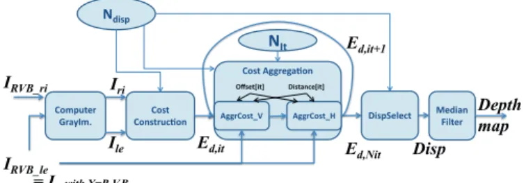
Computer GrayIm. Median Filter Cost Construcion Cost Aggregaion AggrCost_V AggrCost_H Ndisp NIt Iri Depth map Offset[it] Distance[it] DispSelect Ile IRVB_le IRVB_ri Ed,it Ed,it+1 Ed,Nit Disp = Ix with X=R,V,B
Fig. 1: Description of the Stereo Matching Algorithm
B. DSP Core
In this section, the main specific architecture point of c66x cores are introduced.
1) VLIW: The C66x DSP core is able to executes up to 8 instructions simultaneously in one cycle Thanks to Very Long Instruction Word (VLIW).
In most digital signal processing applications, a loop kernel is a succession of interdependent sequential operations. These loops must be pipelined to be parallelized.
Loop pipelining is done by the compiler, and a factor 6 speed-up can be easily achieved with a little human work. However a pipelined loop can not have any jumps, and conditional statements (if/else) must be avoided inside the loop. These rules must be kept in mind when writing efficient code and designing algorithms.
2) SIMD: Single Instruction Multiple Data (SIMD) are instructions that are executed on multiple data. A SIMD instruction considers one or two registers (32 or 64 bits respectively) as a set of smaller words. For instance a 32-bit register can be seen as a group of 4 8-32-bit words, and is called a 4-way 8-bit SIMD instruction.
This kind of instruction is very useful in image processing because most of the manipulated data are 8-bit (pixels).
C. FPU
The FPU (Floating Point Unit) is a logic unit which is able to execute operations on floating point numbers. The c66x has a basic FPU ; Nevertheless, this FPU has low support of SIMD (two ways maximum), whereas SIMD on fixed point numbers is up to 8 ways. Moreover a floating point number is always 4 byte wide, and causes a higher memory usage.
III. PROPOSED ALGORITHM
A stereo matching algorithm computes depth information from two cameras. The goal of these algorithms is to match a pixel in left image with one in the right image. Due to their high computational complexity, designing real time stereo matching algorithms is a great challenge.
In the past decades a lot of work has been done on stereo matching algorithms to increase their quality and time efficiency. There are two main categories of stereo matching algorithms : local and global methods [3].
Global methods minimize global energy on the entire dis-parity map or scanline. Global methods are very good in terms of quality, but not very well suited for real time applications.
Local methods are area-based algorithms, they match pixels by taking into account the neighbourhood of these pixels. Local methods give less accurate results than global methods, but they are much faster.
In this paper, only local methods are considered for real time considerations. The Middlebury Stereo Vision Website [3] is a reference for the comparison of Stereo Matching algorithms. The best ranked algorithms of this database and the related papers has been studied. As the highest ranked algorithm is not published, the algorithm proposed by Mei[4] has been targeted for a DSP Implementation.
First, the original algorithm [4] will be introduced, and all algorithm blocks will be detailed. Then, real time limitations of this algorithm will be discussed and solutions to bypass those limits will be exposed. To finish this section, some implementation details will be given.
A. Algorithm overview
Figure 1 represents the chosen algorithm [4]. It is composed of three main steps :
• The cost construction which computes matching cost for
each possible disparity and for all pixels.
• The cost aggregation which refines those cost maps
thanks to an iterative algorithm.
• The disparity selection which selects the minimum
matching cost (i.e. the best match) and deduces the disparity.
A median filter is applied at the output of the disparity selection step. The median filter is common and will not considered in this paper.
1) Cost construction: The cost construction step takes left and right images and computes a matching cost for all possible disparity levels. Its output is a cost map for each disparity level (same size as input image). It is computed thanks to equation (1).
For a disparity d, a pixel p of coordinates (x, y) is taken in the left image and compared to a pixel pd of coordinates
(x + d, y) in the right image. The result of the comparison is an error that is called matching cost. Equation (1) describes the matching cost that is computed on each pixel and for all possible disparities.
Cost(p, d) = CT AD(p, d).λT AD+ CCEN(p, d).λCEN (1)
Equation (1) is composed of two sub-costs summed to-gether :
• The truncated absolute difference cost (CT AD) expresses
the similarity of two pixels and is described in section III-A1a.λT AD is a weight associated to CT AD cost. • The census associated cost (CCEN) gives an information
about local texture and is described in section III-A1b. λCEN is a weight associated toCCEN cost.
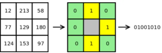
Fig. 2: 8 bits census signature example
a) Truncated absolute difference: The CT AD expresses
the similarity of two pixels, it focuses only on grey levels similarity, and not about its neighbourhood.
CT AD(pd, d) = 1 − e−
|Il(p)−Ir (pd)|
thr (2)
Ir and Il are left and right grey level images. thr is a
threshold (i.e. a constant) which defines the useful dynamics of truncated absolute difference. It must be superior to the noise value in image, 20 is a common value in the literature [3].
b) Census Cost: The census gives an information about local texture that CT AD does not provide.
Census produces an 8-bit signature for each pixel of an input image. As shown in figure 2, this signature is obtained by comparing each pixel to its 8 neighbours. The census is referred ascenl,cenrin equation (3) for respectively left and
right grey level images.
CCEN(p, d) = 1 8 7 X k=0 ( 0 ifcenr(p)[k] = cenl(pd)[k] 1 ifcenr(p)[k] 6= cenl(pd)[k] (3)
In equation (3), CCEN is the cost associated to census.
cenl(p)[k] and cenr(p)[k] are the kth bits of the 8-bit census
signature for pixel p in the left and right images respectively. pd is the pixel of coordinatesp − d, with d the disparity level.
Equation (3) is a sum of bit-to-bit comparisons, and these bit-to-bit comparisons are equivalent to a boolean operation called ”exclusive or” (XOR).
The output of the cost construction step is one cost map per disparity level. Those cost maps are the input of the cost aggregation step.
2) Cost aggregation: The cost construction step has a low computing cost, but it provides noisy matching cost maps. This noise is mainly produced by CCEN which is random when
compared regions are not correlated. To remove this noise, the cost aggregation step performs smoothing on areas with similar colour in the original image. The cost aggregation step is performed independently on each cost map. This is a key point regarding implementation.
The cost aggregation algorithm’s structure is similar to a bi-lateral filter. The cost aggregation step is performed iteratively with varying parameters, it is defined by equation (4).
Ei+1(p) = W (p, p+)Ei(p+) + Ei(p) + W (p, p
−)Ei(p−)
W (p, p+) + 1 + W (p, p−)
(4)
Ei is the current cost map to be refined, E0 is the output
of cost construction (equation (1)).
Pixelsp+ andp− have a position relative to pixelp : • p+= p + ∆i
• p−= p − ∆i
Equation (4) is computed alternatively for horizontal and vertical aggregation :
• Wheni is odd, it is a vertical aggregation, the offset ∆i
is vertical.
• Wheni is even, it is a horizontal aggregation, the offset
∆i is horizontal.
At each iteration the parameter∆igrows, thus further pixels
p+ andp− are used for smoothing p. ∆i evolves according
to equation (5), the influence range is limited by the modulo (here∆i∈ [0, 32]).
∆i= f loor(i/2)2mod 33 (5)
WeightsW in equation (4) are defined by equation (6) :
W (p1, p2) = eCd.∆i− sim(p1,p2) L2 (6) sim(p1, p2) = s X col∈(r,g,b) (Ircol(p1) − Ircol(p2))2 (7)
In equation (6),Cd is a weight applied to distance[4] and
L2 is the weight applied to similarity [4]. Ir{r, g, b} and
Il{r, g, b} are the RGB (Red, Green, Blue) signals of right
and left images.
3) Disparity selection: The disparity selection step min-imizes the matching cost. To do so, the Winner Takes All (WTA) strategy [3] is applied. The WTA strategy is a simple arithmetic comparison expressed by equation (8).
Disp(p) = argmin
d∈[0,N disp]
Ed,N it(p) (8)
The output of disparity selection is a dense integer disparity map providing a disparity value for each pixel in the right image.
B. Arithmetic simplification
Section III-A has exposed the original algorithm. Now the proposed modifications in order to speed up the algorithm without too much degradation are exposed.
To be fast, all algorithm blocks must be implemented in fixed-point arithmetic, because the DSP is more efficient with fixed points (see II-C).
To be easily implemented in fixed-point arithmetic all functions must be described with classical operators (+, −, ∗). Functions such as square root or exponential must be avoided. These principles are applied in the proposed modifications below.
1) Cost construction: Section III-D2 will show thatCCEN
fits well on a DSP architecture. ButCT ADshould be simplified
(exponential function is not recommended). A common way in the literature [3] is to use a raw saturation described by equation (9).
CT AD(i, j, d) = min(thr, | Iri(i, j) − Ile(i − d, j) |) (9)
Equation (9) is used instead of equation (2).
2) Cost aggregation: Cost aggregation takes up 85 % of execution time (weight and aggregation rows in table III). Optimization of cost aggregation is thus most important in the stereo matching algorithm.
a) Number of iterations: The cost aggregation execution time being linear with respect to the number of iterations, a way to reduce execution time is to reduce the number of iterations. This point will be explored in section II.
b) Weight computing: Weight computing is quite com-plex because of the exponential function and the square root in equation (6). In this equation, the weights increase when two pixels are similar and decrease with distance. Equation (10) proposes a piecewise linear function to approximate equa-tion (6).
W (p1, p2) = thr − truncthr(sim(p1, p2))
thr .(1−∆.Cd) (10) Equation (11) avoids use of square root by using a norm L1 instead of a normL2 in the original equation (7).
sim(p1, p2) = X
col∈(r,g,b)
| Ircol(p1) − Ircol(p2) | (11)
In equation (10), the denominator of the division is a constant and thus can be replaced by a multiplication by1/thr.
c) Aggregation: The core of cost aggregation is a simple weighted sum (numerator of equation (4)). The denominator of equation (4) expresses a normalization.
The normalization is important because it prevents diver-gence and keeps a constant average cost value. A constant average value is necessary because of the lack of signal dynamic due to fixed point. To reach this goal, the sum of weights must be equal to one.
This normalization is a critical point because it implies a division which is not handled by the hardware.
The proposed approximation to normalization is described by equation (12). The wanted property, the fact that the sum of weights equals one, is verified by equation (12) (W p + W m + W o = 1). W p = W (p, p+) 4 W m = W (p, p−) 4 (12a) W o = 1 − (W p + W m) (12b) Eit+1(p) = W p.Eit(p+) + W o.Eit(p) + W m.Eit(p−)
(12c) Equation (12) uses only basic operators : +, −, ∗ and ≫ (shift right) for the division by 4.
C. Memory optimization
The main difficulty of implementation in embedded systems is the efficient use of the memory architecture. Data in the slow external memory (DDR3) should be avoided (see II-A). Best performances are reached when the memory footprint is lower than the internal memory size in order to bypass the external memory. The memory footprint of the algorithm has to be reduced. Next sections describe the proposed strategies to reduce memory footprint.
1) Disparity selection: Cost construction and cost ag-gregation are done independently for each disparity level (equations (1) and (4)). Winner Takes All (WTA) strategy (equation (8)) finds the minimum value of their outputs.
It is not necessary to store each level of disparity in memory when implementing argmin on the fly. Only the cost of the current disparity level (Ed), the current argmind and
minimum values (mind) have to be kept in memory.
2) Weight precomputing: The iterative equation (12) is the core of this algorithm. Weights are independent of disparity but they are dependent on∆i (see equation (10)). That is why
weights can be precomputed and reused for each disparity level.
Moreover, memory and computational complexity can be avoided. Indeed equation 11 implies W (p1, p2) = W (p2, p1) which also implies thatW (p, p+) and W (p, p−) are identical
with an offset of ∆i. This can easily be proved by taking a
second point p′
in weights table that has an offset of∆i :
p′
= p + ∆i= p+ p′−= p ′
− ∆i= p
W (p, p+) = W (p+, p) = W (p′, p′−)
Because the tables W (p, p+) and W (p, p−) are identical
with an offset of∆i, only one of them needs to be computed.
This property decreases memory requirement and computation by a factor two when precomputing weights.
Two weights tables are required per value of∆i (one
hori-zontal and one vertical). Using this precomputing, each pixel operation is reduced to three additions and two multiplications plus normalization (see III-A2).
Finally all memory optimizations lead in a 13 times smaller memory footprint (for a 20 disparity level image) :
• A factor 4 is obtained by replacing floating point by fixed
point.
• Precomputed weights take 2 buffers per iteration level
instead of 6.
• It is no more necessary to store each disparity level in a
buffer.
D. Hardware optimization
Previous parts were dealing with generic optimizations ;in this part, c66x-specific hardware optimizations are introduced. As explained in section III-B, a set of basic operators must be used (+, −, ∗). Those operators are available on all platforms, and often in SIMD version. But the c66x DSP has special instructions that are very useful for this application.
The following sections describe how to use these instructions efficiently.
1) Truncation: In part III-B, some truncation (minimum) functions were used (in equations (9) and (10)). The DSP has a 4-way 8-bit SIMD minimum instruction (minu4[5]), so any saturation function can be implemented very efficiently without any conditional statement, thus this implementation is compatible with loop pipeline (see II-B1).
2) Census: The census cost is implemented very efficiently using special instructions.
When looking at the description of the census cost in section III-A1b, it cannot be implemented with usual operators, and might look hard to implement. But there is a very efficient implementation on the c66x DSP.
First, comparisons with a pixel’s neighbourhood are not a problem, because they are precomputed once, and the cumulated execution time is negligible.
Second, an exclusive or can be used to compare the two 8-bit signatures in Equation (3). To count the number of bits that are equal to one, the ”bit count” instruction can be used efficiently. This instruction takes a word and returns the number of bit which are equal to one. This instruction is available on 4-way 8-bit SIMD (bitc4[5]).
IV. RESULTS
This section exposes the results of the proposed modifica-tions in quality and performance (execution time). The fixed point implementation introduces more computing noise, thus the quality loss due to fixed point must be quantified.
A. Quality Assessment
The quality of algorithm output has been evaluated with Middlebury evaluation tools [3]. The Middlebury evaluation gives the number of bad pixels in different parts of the image. In this paper two values are considered for quality assessment:
• The global number of bad pixels. It gives a good
repre-sentation of the overall image quality.
• The number of bad pixels in non-occulted areas of the
image. This algorithm does not deal with occulted areas, and the disparity map on those areas is very noisy, thus results on occulted areas are partially random. Comparing random results together does not give clear results. That is why, when comparing two versions of this algorithm, it is better to look at non-occulted parts of images.
1) Data Set: Seven images from the Middlebury database [3] are used to evaluate quality for the proposed algorithm (Aloe, Art, Laundry, Map, Sawtooth, Tsukuba, Venus).
2) Algorithm parameters: The algorithm’s default constants from the literature are used [6], [7], [3]. These constants have not been tuned to increase quality on this particular data-set :
• thr in equation (9) : 20 • thr in equation (10) : 60 • Cd in equation (10) : 0,015 • λcen in equation (1): 0,55 • λtad in equation (1) : 0,45
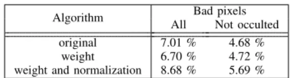
TABLE I: Quality of algorithms
Algorithm Bad pixels All Not occulted original 7.01 % 4.68 %
weight 6.70 % 4.72 % weight and normalization 8.68 % 5.69 %
TABLE II: Influence of iterations on cost aggrega-tion.
Iteration steps (∆i) Iterations Bad pixels
All Not occulted 1, 4, 9, 25 4 7.6 % 5.1 % 1, 4, 9, 16, 1 5 7.7 % 5.3 % 1, 4, 9, 16, 25 5 7.1 % 4.9 % 1, 4, 9, 16, 25, 3 6 6.7 % 4.7 % 1, 4, 9, 16, 25, 36 6 6.6 % 4.7 % 1, 2, 4, 8, 16 5 7.8 % 5.4 % 1, 2, 4, 8, 16, 32 6 6.7 % 4.6 %
B. Impact of approximations on quality
Impact of approximations described in part III-B on quality are exposed in table I.
The impact of weights and cost construction approximation on quality is 0.04 % on non-occulted pixels, and it can be considered as negligible. This can be explained by the fact that the equation (11) describes correctly the similarity of two pixels. Moreover, because outputs of those functions are only used for arithmetic comparisons in disparity selection (see equation (8)), impact on quality is minor. Since functions are monotonic (if arithmetic precision is not taken into account). The normalization approximation is very intrusive, the qual-ity loss is expected to be important on this point. Indeed the normalization approximation (equation (12)) degrades the quality by 1 % (see table I) on not occulted pixels, this is an acceptable quality lost.
C. Cost aggregation iterations
As explained in part III-B2, a easy way to increase perfor-mance is to reduce the number of iterations. Table II exposes the impact of number of iterations and the value of ∆i on
quality. The more iterations there are the better the quality is. But with more than four iterations, the quality does not increase very fast. This can be explained by the iterative algorithm which makes the result tend to an optimal value.
The execution time is almost linear with respect to the number of iterations. The sixth line of table II is a good trade-off between the number of iterations and quality.
(a) input pictures (b) Original (c) Proposed
TABLE III: Execution times on DSP.
algorithm step execution number floating point fixed-point pipeline SIMD aggregation N it.N Disp(95) 13,24 30,13 % 8,83 75,80 % 1,44 63,58 % 0,41 56,72 % cost construction N Disp(19) 100,09 45,56 % 5,44 9,34 % 1,89 16,72 % 0,63 17,40 % disparity N Disp − 1 (18) 1,56 0,23 % - 2,54 % - 13,04 % 0,20 5,12 % weight N it(5) 199,73 23,92 % 19,37 8,75 % 1,93 4,48 % - 13,97 % total (FPS) 0,24 0,9 4,7 * 14,5 * : data not directly measured (computed from measured values). - : not implemented parts. Units are machine million cycles (The DSP is clocked 1 GHz, 1 million cycles = 1 millisecond).
TABLE IV: Sawtooth quality
Algorithm Bad pixels All Not occulted original 2.43 % 1.12 % normalization 3.41 % 1.35 % DSP (SIMD) 4.02 % 1.68 %
D. Fixed point precision
When implementing on the DSP using SIMD, some signif-icant bits are removed to increase speed. Table IV exposes the quality lost when porting on DSP.
Results of only one image on DSP is presented, the quality loss is the same for others images. Indeed the quality loss is only due to precision lost on the DSP, and the loss is the same magnitude for any image. Results of image sawtooth are exposed in table IV.
The quality degradation from line 2 to 3 of table IV is caused by the reduction of arithmetic precision to enhance the speed of SIMD instructions. When using 8-bit data instead-of 16-bit data, twice as many operations can be achieved in one SIMD cycle.
Table IV shows a 0.5 % quality degradation caused by the loss of arithmetic precision. This quality degradation is not prohibitive. The stereo pair and output disparity map are shown figure 3.
E. Speed
In previous sections, the quality lost due to optimizations and arithmetic simplifications has been exposed. This last section deals with the speed performances resulting from those simplifications.
Table III shows execution time of each algorithm step, and the percentage of time used by these steps. The original version of the algorithm (floating point) runs at 0.24 fps on DSP, the fully optimized version runs at 14.5 fps, the speed-up factor is 60. Disparity selection step uses inherently fixed point (deals with integer disparity value), thus it is tagged as not implemented in fixed-point column. Disparity selection step can not benefit of loop pipeline without SIMD implementation, thus it is tagged as not implemented in pipeline column. Some steps were not optimized with SIMD because their execution times are too small to have a significant impact on total execution time.
Proposed modifications in section III are introduced at fixed-point column of table III. However, speeds of pipelined and SIMD versions could not be reached without proposed
optimizations. For instance, as explained in section III-B2c, the cost aggregation core could not be pipelined because of normalization. That is why the speed-up of proposed modi-fications is not reduced to the speed-up between the original algorithm and its fixed point version.
To conclude this section on performance, the proposed modifications lead to a factor 60 speed-up (table III) with a quality of 8.68 % (table I) of bad pixel on image compared to 7.01 % before modification.
V. CONCLUSION AND PERSPECTIVES
The goal of this paper was to prove the feasibility of real-time dense stereo matching on a DSP platform. Currently, a cost-aggregation based algorithm is running at 14.5 fps on one c66x core. This speed has been reached with minor quality loss.
If the quality degradation is too important for applications, a trade-off depending on application can be found to increase quality. More significant bits can be allocated for computing with a quality improvement, but less operations can be done simultaneously, and eventually, more memory would be used (if intermediate data are store to 16 bits instead of 8). Moreover an easy way to increase the quality is to increase the number of iterations in the cost aggregation core.
The current implementation of the algorithm described in this paper uses only one of the eight cores of the c6678 platform. Future work will consist in using all the cores of this platform.
REFERENCES
[1] E. V. Alliance, “What is embedded vision.” http://www.embedded-vision. com/what-is-embedded-vision.
[2] K. Khoshelham and S. O. Elberink, “Accuracy and resolution of kinect depth data for indoor mapping applications,” Sensors, vol. 12, no. 2, pp. 1437–1454, 2012.
[3] R. S. Daniel Scharstein, “A taxonomy and evaluation of dense two-frame stereo correspondence algorithms,” International Journal of Computer
Vision, no. 47, pp. 7–42, 2002.
[4] X. Mei, X. Sun, and M. Zhou, “On building an accurate stereo matching system on graphics hardware,” in Computer Vision Workshops (ICCV
Workshops), 2011 IEEE International Conference on, nov. 2011, pp. 467 –474.
[5] TMS320C66x DSP, CPU and Instruction Set, Texas Instruments. [Online]. Available: www.ti.com/lit/ug/sprugh7/sprugh7.pdf
[6] A. Mercat, J.-F. Nezan, D. Menard, and J. Zhang, “Implementation of a stereo matching algorithm onto a manycore embedded system,” pp. 1296–1299, June 2014.
[7] J. Zhang, J.-F. Nezan, M. Pelcat, and J.-G. Cousin, “Real-time gpu-based local stereo matching method,” in conference on Design and Architecture