HAL Id: hal-01635393
https://hal.archives-ouvertes.fr/hal-01635393
Submitted on 23 Nov 2017
HAL is a multi-disciplinary open access
archive for the deposit and dissemination of sci-entific research documents, whether they are pub-lished or not. The documents may come from teaching and research institutions in France or abroad, or from public or private research centers.
L’archive ouverte pluridisciplinaire HAL, est destinée au dépôt et à la diffusion de documents scientifiques de niveau recherche, publiés ou non, émanant des établissements d’enseignement et de recherche français ou étrangers, des laboratoires publics ou privés.
Creation of a corpus of realistic urban sound scenes with
controlled acoustic properties
Jean-Rémy Gloaguen, Arnaud Can, Mathieu Lagrange, Jean François Petiot
To cite this version:
Jean-Rémy Gloaguen, Arnaud Can, Mathieu Lagrange, Jean François Petiot. Creation of a corpus of realistic urban sound scenes with controlled acoustic properties. 173rd Meeting of the Acoustical Society of America and the 8th Forum Acusticum (Acoustics’17), Jun 2017, Boston, MA, United States. pp.1266-1277, �10.1121/2.0000664�. �hal-01635393�
Proceedings of Meetings on Acoustics
Creation of a corpus of realistic urban sound scenes with controlled acoustic properties
--Manuscript
Draft--Manuscript Number:
Full Title: Creation of a corpus of realistic urban sound scenes with controlled acoustic properties Article Type: ASA Meeting Paper
Corresponding Author: Jean-Remy GLOAGUEN, Ph. D. Ifsttar
Bouguenais, Pays de la Loire FRANCE Order of Authors: Jean-Remy GLOAGUEN, Ph. D.
Arnaud Can Mathieu Lagrange Jean-François Petiot
Abstract: Sound source detection and recognition using acoustic sensors are increasingly used to monitor and analyze the urban environment as they enhance soundscape
characterization and facilitate the comparison between simulated and measured noise maps using methods such as Artificial Neural Networks or Non-negative Matrix Factorization. However, the community lacks corpuses of sound scenes whose acoustic properties of each source present within the scene are precisely known. In this study, a set of 40 sound scenes typical of urban sound mixtures is created in three steps: (i) real sound scenes are listened and annotated in terms of events type, (ii) artificial sound scenes are created based on the concatenation of recorded individual sounds, whose intensity and duration are controlled to build scenes that are as close as possible to the real ones, (iii) a test is carried out to validate the level of their perceptual realism of those crafted scenes. Such corpus could be then use by communities interested in the study of the urban sound environments. Section/Category: Signal Processing in Acoustics
1. INTRODUCTION
The urban sound environment is studied both from the perceptual1,2 and from the physical point of view3.4 These studies can be based on real sound environments either by acoustic listening through a sound-walk5or with recordings made in city,6or by using sound mixtures resulting from a simulation process.7In the first case, since it has an undeniable ecological validity, it doesn’t make it possible to have a repeatable experience nor to propose a controlled framework where the presence and the level of the different sound sources can be adjusted. Then the use of a simulation tool to create specific urban sound environments is a useful way to control the degree of contribution of each class of acoustical sources. It allows us to create urban sound environments by adjusting some parameters8or to assess performances of some classification9 or source separation tools.10
A critical question is then to obtain scenes that are realistic enough to be considered as similar to refer-ence recordings. To do so, various methods have been proposed. The first approach would be to simulate completely a neighborhood taking into account the architecture of the buildings, the sound dynamics of the different sources present (car, voice, bird, bell . . . ) and their propagation to a receptor, as proposed by.11 If the first renderings are interesting, this method remains complex to implement with results that are still too artificial. A more straightforward approach composes sound mixtures from isolated sounds mixed to-gether. The idea is to consider the urban sound environment as the sum of acoustic events, i.e. events with a sufficient sound level to be discernible, superposed to a sound background, i.e a sound constant on the sound mixture whose properties vary slowly during the scene. The difficulty here is to have a representative database of isolated sounds with a sufficient quality to not compromise the resulting sound quality and to sequence the acoustic events wisely.
The method proposed by Misra & al.12 enables to resolve the first issue by extracting the acoustical events directly in real recordings and by manipulating them to re-use them in new mixtures. Since the tool has a sufficient number of parameters to control the sound event, their method is limited by the extraction phase: the overlapping between the acoustic events deteriorates the sounds and then the final rendering. Furthermore, the manipulations (duration, frequency range) can create artifacts that can deacrease the real-ism. In a similar way, the tool proposed by Davis and Bruce8 enables to compose sound mixtures with an isolated sound database composed of recordings made specially for their application. The creation of the urban sound mixtures is made possible with the perceptual assessment of a panel of listeners of the different sound environments. This method enables to determine which sounds are the most representative or the most linked to an urban sound environment from a perceptual point of view.
However, as our objective here is to get simulated scenes that are as realistic as possible, this method can not be considered because if this method proposes a perceptual validity, it can not provide an ecological one. Thus, this study proposes to create urban sound mixtures from the listening of urban audio recordings and the estimation of some high level sequencing parameters extracted from the recordings to tune an audio simulation tool. The realism of the simulated scenes is then assessed using a perceptual test.
The remaining of the paper is organized as follows: Section 2 focuses on the study of recordings made in Paris, Section 3 deals with the simulation tool and Section 4 summarizes the results obtained in the perspective test.
2. STUDY OF REAL SCENES
Real urban noise recordings are listened in details to determine the composition of typical urban sound environments in terms of sound sources, presence and level. The recordings considered in this study have been made on the 13th district of Paris (France) as part of the GRAFIC project13during a soundwalk which was designed to cover different types of urban sound environments.
Figure 1: Map of the soundwalk with the 19 stop points
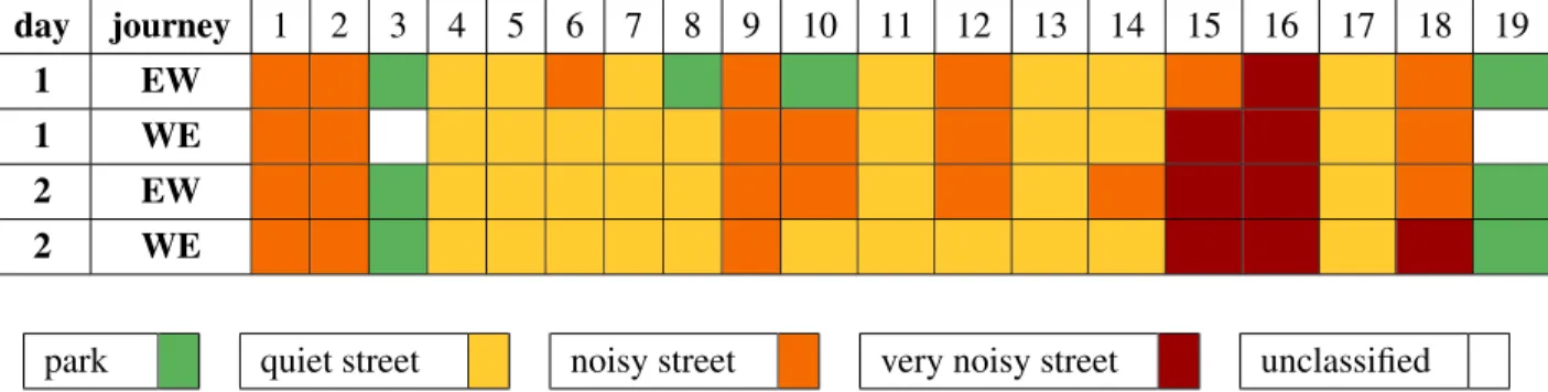
The walk was 2.1 km long, consisting of 19 stop points with a recording duration between 1 to 3 minutes (see figure 1). It was roamed on two days (03/23/2015 and 03/30/2015), twice a day (on the morning and on the afternoon) and in one direction (from West to East, WE) and then in the other (from East to West, EW). The acquisition system used was a ASAsense and was carried on the backpack of the operator which was walking with the participants. In the end, 76 (4 × 19) audio files (sampled at 44,1 kHz) were available and serve as a basis for the study. More details can be found on.14 Each file is fully annotated in terms of sound classes that are present in the urban area and their recurrence. It is labeled using the following types of sound environments (park, quiet street, noisy street, very noisy street) as proposed by15or3(Table 1).
day journey 1 2 3 4 5 6 7 8 9 10 11 12 13 14 15 16 17 18 19
1 EW
1 WE
2 EW
2 WE
park quiet street noisy street very noisy street unclassified
Table 1: Classification of the scenes according to the sound environment
Most of the scenes of the recordings belong to quiet street and noisy street. 2 scenes are removed form the database: a noisy cleaning truck is present inside the 1-WE-03 heavily polluting the sound scene and the 1-WE-19record is too short to be considered in this study. From the annotations, each sound environment is characterized by the sound classes present in the recordings. The most recurrent sound classes are presented in Table 2.
As the calibration audio file was not available, the sound level cannot be considered as absolute but the relative difference between each sound environment can be considered. The road traffic, the voice and the bird components are the most discriminant classes of the sound environment: with exclusively road traffic, the noisy and very noisy sound environments are different to the park and quiet street where the voice and the bird’s whistles are predominant. Furthermore, multiple sound classes can be heard whatever the urban sound environments : dog barks, church bell ringing, car horn, sirens . . . with a density that can be very low (< 0.1/min). Finally, a lot of brief sounds with unknown origin can be listened in almost all the files. Consequently, all these indefinite sounds are annotated in one unique class sound, street noise. From this information (density, level, sound classes present in each sound environment), it is now possible to compose
Sound environment Sound level (dB) Background Event number events/min Park 69.0 voice, bird’s whistles road traffic voices bird’s whistle street noise foot step 0.5 0.5 0.5 0.5 0.3
Quiet street 70.2 road traffic
bird road traffic voices street noises foot step bird construction site noise door house door car 1.0 0.7 0.7 0.5 0.2 0.1 0.2 0.2
Noisy street 73.5 road traffic
traffic foot step voice street noise bell bird car horn car’s door siren 9.0 0.5 0.6 0.4 0.1 0.2 0.3 0.2 0.1 Very noisy
street 76.0 road traffic
traffic voice siren car horn bird foot step car’s door street noise 40 0.3 0.2 0.3 0.2 0.3 0.2 0.3
Table 2: Sound level and description of the most recurrent sound classes (backgrounds and events) present in the sound environments
3. SIMULATION OF REALISTIC AUDITORY URBAN SCENES A. PRESENTATION OF THE WEB-SIMULATOR SIMSCENE
simScene16 is a simulator that creates sound mixtures in a .wav format by superposing audio samples that come from an isolated sound database composed of two categories: the brief sounds (from 1 to 20 seconds) that are considered as salient belong to the event category whereas all the sound that are of long duration and whose acoustic properties do not vary with respect to time belong to the background category. Inside each category, the sound samples are then grouped in sound classes (bird, car, foot steps . . . ). The software enables the user to control for each sound class some parameters as the number of events of each class that appears in the mixture, the elapsed time between each sample of a same class or the existence of a fade in and a fade out . . . . Each parameter is completed with a standard deviation that may brings some random behavior between the scenes.
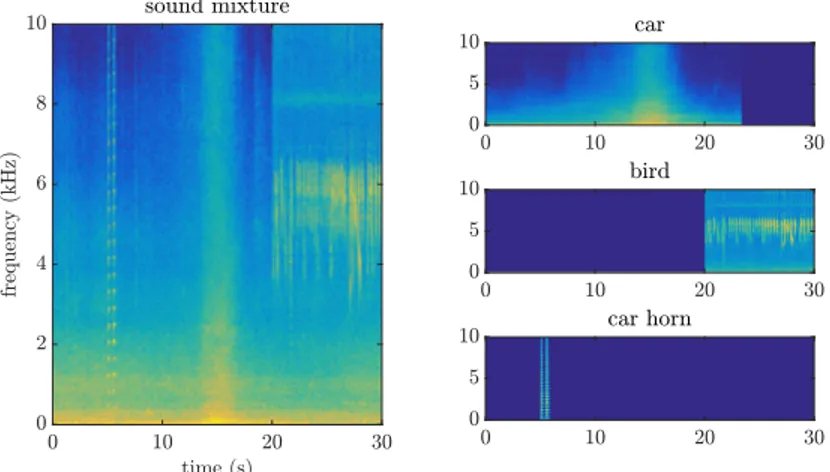
Figure 2: Example of a scene composed of three sound classes
The sound mixtures can be created following two modes: the abstract mode allows to create mixtures from the specified parameters while the replicate mode reproduces an existing scene by following as much as possible its annotation file. With the audio file of the global sound mixture, each sound class can be resumed in a separate audio file, which allows to know their exact contribution in the scene.
B. CREATION OF THE URBAN SOUND DATABASE
Based on the annotations of the 74 real scenes, a sound database is built with sounds found online on the freesoundproject and with the help of the urbanSound8k database.17 This database consists in more than 8000 files with a 4 seconds or less duration, found on the web site freesound.org too, and classified in 10 sound classes: ventilation, car horn, children playing, dog barking, bell, engine idling, gunshot, jackham-mer, siren and street music. All the audio files have been sorted and those who presented the best signal to noise ratio have been selected.
In addition, as road traffic is a prime audio source in an urban sound environment, it seemed interesting to have, in the database, a part composed of well-recorded car sounds. As a result, passages of 4 differ-ent cars (Renault Scenic, Clio, Megane and Dacia Sandero) were recorded on the Ifsttar-Nantes reference test track at different speeds and gear ratios for steady, acceleration, braking (Table 3) and stopped phases. Among the 108 recordings planned, those for the acceleration and braking phase for the Renault Senic could
not be done whereas some recordings have been made twice for the other vehicles. In all, 103 car passages have been recorded.
Trans. 1 2 3 4 5 stabilized speed (km/h) 20 × 30 × × 40 × × × 50 × × 60 × × 70 × × 80 × 90 × braking acceleration speed (km/h) gear r. speed (km/h) gear r. 50 → 0 3 → 2 0 → 30 1 → 2 40 → 0 2 → 2 0 → 40 1 → 2 50 → 30 3 → 2 20 → 40 1 → 3 60 → 40 4 → 3 30 → 50 2 → 3 70 → 50 4 → 3 40 → 60 3 → 4 80 → 50 4 or 5 → 3 50 → 70 3 → 4 or 5
Table 3: Description of the recordings set on runway with vehicle passages with stabilized speed (left) and in acceleration and braking phase(right) with different gear ratios
To obtain the cleanest possible sound samples, a median filter18 has to be applied to filter out bird’s whistles present in the recordings. The filter consists in taking a window around a center point and to attribute to it the median value of this window. This method allows to attenuate the brief variations both in the spectral and the temporal plan. The size of the filter window is chosen with a 5 points width and a 9 points height in the frequency range [2500 − 6500] Hz, so that the effect of the filter is sufficient without deteriorating the quality of the audio (see Figure 3).
Figure 3: Spectrogram in the frequency range [2500 − 6500] Hz of a recorded passage of the Renault Megane car at 40 km/h with the 3rd gear ratio (Nw = 212with 50 % overlapping, Nf f t = 212, sr = 44.1
kHz). On the left, the original recording, on the right, the filtered audio with the filtered part.
Finally, the resulting database is composed of 245 sound events (bell, whistle bird, sweeping broom, car horn, car, hammer and drill, coughing, dog barking, car and house door slamming, plane, siren, foot step, thunder, street noise, suitcase rolling, train and tramway passing, truck and voice) and of 154 background sounds (birds, construction site, crowd, park, rain, schoolyard, traffic, ventilation, wind).
The simulated sound scenes have, in consequence, the same temporal structure than the real scenes. The main difficulty is then to adjust correctly the sound level of the events to be faithful compared to the real scenes. In order to obtain a corpus of urban sound scenes, resulting from a simulated process and sufficiently realistic, a perceptual test is set up to assess the realism on several of them.
4. PERCEPTUAL TEST A. DESIGN OF THE TEST
A perceptual test is conducted with a panel of listeners that are asked to assess the level of realism on a 7-point scale (1 is not realistic at all, 7 is very realistic) of an auditory scenes, recorded and simulated. The total number of sound scenes to be tested is set at 40. The first half includes 20 30-seconds audio files, blending of 5 scenes that belong to the sound environment Park, 6 from Quiet street, 4 from Noisy street and 5 from Very noisy street chosen randomly among the 74 recorded scenes. Then, the second half is composed of the same 30-second audio samples from the replicated scenes. In order to limit the duration of the test and to preserve the concentration of the subjects, each subject listens a subset of 20 sound scenes (10 real sounds scenes and 10 replicated). Furthermore, to prevent the listeners from changing the sound level of their speakers, all the scenes are normalized to the same sound level, chosen at 65 dB.
The experimental design is elaborated following a Balanced Incomplete Block Design (BIBD)19where J participants make K assessments from B sound scenes, each of them are tested R times and each couple of sound sources are presented λ times in one block. In order to have BIBD, a 3 rules govern these parameters : B ≥ K, J K = BR, λ = RK − 1 B − 1. (1a) (1b) (1c)
with [J, B, K, R, λ] ∈ N. A reasonable number of listeners is chosen at J = 50. With theses parameters fixed, J = 50, K = 20, B = 40 and R = 25, the BIBD is not fully balanced (condition (1c) /∈ N). It is finally with a partially BIBD that the listening plan is elaborated.20 It consists, with the parameters J , K and R fixed, in determining the optimal plan that would be the most balanced. The package sensoMineR on the Rsoftware provides the plan where the listening order per participant is defined inside.21 As the distribution of the simulated and real samples for each participant is almost identical, the obtained listening plan can be considered as balanced (Figure 4).
The test was administered online1on the 8 February 2017 and the number of 50 participants has been reached 12 days later. During the test, the participant had the possibility to listen to each scene as many times as wanted before assessment it, without being able to change his/her judgment afterwards. The participant could also leave a comment on each audio to explain the rating. Finally, the age, gender and experience on listening to urban sound mixtures were asked at the end of the test. The panel of 50 listeners was made of 31 males and 18 females (one not documented) with an average age of 36 (± 12) years old. 62% of the participants declared having no experience in the listening of urban sound mixtures.
1
Figure 4: Distribution between the real and simulated scenes for each participant. The cumulative sum is equal to the number of tested elements K.
B. RESULTS
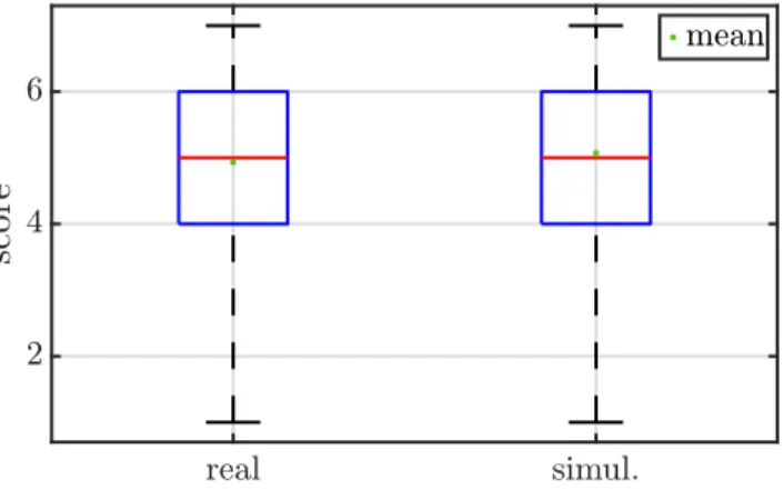
First, the note distributions are represented by a box-and-whiskers plot according to whether they be-longs to the type real or simulated.
Figure 5: Box-and-whiskers plot of the rating of realism according to the type of scene
The distribution allow to considered that the notation given the subjects are extremely similar. One can note that the mean for the simulated scene is even superior to the real one (msimul. = 5.1(±1.6),
mreal= 4.9(±1.6)).
The paired samples t-test is then performed to validate the similarity between the two types. It consists in validate (or not) an H0hypothesis which considers the similarity between the distribution of the average
scores for the recorded and the simulated scenes of each participant with a Student test. This test establishes a p-value that is compared to a threshold value α of 5%. The H0hypothesis is then considered if p−value >
α. The results of the t-test (degrees of freedom (DOF), the absolute value t and p-value) are sum up in the table 4.
DOF | t | p-value
type 49 1.37 0.17
Table 4: Student’s t-test performed on the distribution of the average scores for the recorded and simu-lated scenes
The p − value is calculated at 0.17 > α, which confirms that all the real and simulated scenes are perceived in a similar way by the panel.
From this global result, a first analyze of variance (ANOVA) is performed to determine if the experience in the listening of urban sound mixtures is an influential factor to distinguish real and replicated scenes. In a similar way than the t-test, but based on a Fischer’s statistics, an ANOVA allows to determine if the distri-bution and the interactions of different levels of multiple factors are similar. Therefore, a two-way ANOVA with interaction with the factors ’experience of the panelist in the listening of urban sound scene’ (yes or no) and ’type of scene’ (real or simulated) is carried out. The DOF, the Fisher statistics and the associated p-valueare given in Table 5.
DOF F-statistic p-value
type 1 0.59 0.44
experience 1 1.97 0.16
type/exp. 1 2.14 0.14
Table 5: Two-ways ANOVA with the factors ’type of sound’ and ’listener experience’.
The effect of each factors and the interaction between them are not significant (p-value > 0.05). This means that even listeners trained to hear urban sound environments do not dissociate the real scenes from the simulated scenes better than the non-experienced listeners.
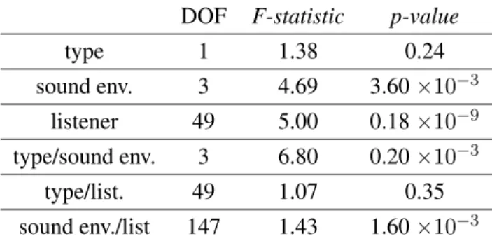
The effect of the ’scene type’, the ’sound environment’ and the ’listener’ factors and their interactions are then studied in a three-ways ANOVA (data distributions displayed on Figure 6 and results in Table 6).
DOF F-statistic p-value
type 1 1.38 0.24 sound env. 3 4.69 3.60 ×10⁻³ listener 49 5.00 0.18 ×10⁻⁹ type/sound env. 3 6.80 0.20 ×10⁻³ type/list. 49 1.07 0.35 sound env./list 147 1.43 1.60 ×10⁻³
Table 6: Three-ways ANOVA for the ’type of sound’, ’sound environment’ and ’listener’ factors with the interaction effects
Again, the ’type’ factor is not influential in the distribution of the notes (p − value > α) whereas the ’listener’ and the ’sound environment’ factors are. There are more variability between the different
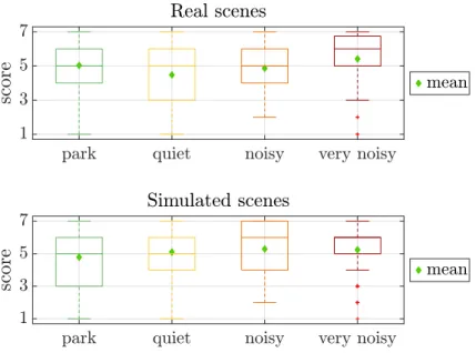
Figure 6: Data distribution according to the ’scene type’ and ’sound environment’ factors
participants or between the different sound environments than between the real and the simulated scenes. But most of all, interactions effects occur for the sound environment with respectively the ’type’ factor and the ’listener’ factors. The interaction effect can be easily illustrated for the case of the ’type’ and ’sound environment’ factors (figure 7). This reveals that the evolution of the perception of realism is not the same according to the sound environment.
Figure 7: Interaction of the two factors ’type of sound’ and ’sound environment’
For the quiet and noisy sound environments, the mean scores increase when the scenes are simulated whereas for it decreases for the park and very noisy sound environments.
One notices, on the simulated scenes, that the park mean score is lower than the other sound environ-ments. In the view of the comment left, it seems that the sound level of the sound classes of foot step and birdsare too loud decreasing the realism of the scores. In a similar way, in the real scenes and particularly in quiet street, it is still the presence of too loud birds and some street noises with unknown origins that have
been remarked by the panelist and have degraded the assessment.
5. CONCLUSION
In order to study the acoustic properties of the urban environment, the research community designs tools that have to be assessed to demonstrate their merit. The availability of simulated scenes realistic enough with precise annotation in terms of content and level will foster research in this direction.
To do so, realistic urban sound mixtures have been composed from the analysis of urban recordings. A work of annotation has allowed to extract, for different acoustic atmospheres, some useful information as the sound classes presence, the traffic flow rates, the sound level. From these observations, a database of urban sound has been created including multiple sound classes both for the sound events and backgrounds. For this study a set of controlled car passages with good sound quality has been recorded. A perceptual test has been set up to quantify the level of realism of the simulated scenes and has revealed that they are comparable to the recorded scenes. Then, the different ANOVA performed have demonstrated that, according to the participants and, most of all, to the sound environment factors, they may still be differences in the distribution of scores. In the case of the simulated scenes, the test enables to reveal that, in the park environment, some sound events (bird and foot steps) must be adjusted to improve the quality of the sound mixtures.
This solved problem, databases of sound sources and urban scenes can be shared with communities interested in performing perceptual tests or in methods of recognizing or detecting sound sources in urban sound environments to help them develop methods.
6. ACKNOWLEDGEMENTS
We would like to thank Pierre Aumond and Catherine Lavandier from the University of Cergy-Pontoise for transmitting us the data of the Grafic project.
REFERENCES
1J. Jin Yong, H. Joo Young, and L. Pyoung Jik. Soundwalk approach to identify urban soundscapes
individually. The Journal of the Acoustical Society of America, 134(1):803–812, 2013.
2D. Botteldooren, C. Lavandier, A. Preis, D. Dubois, I. Aspuru, C. Guastavino, L. Brown, M. Nilsson,
and T. Andringa. Understanding urban and natural soundscapes. In Forum Acusticum, pages 2047–2052. European Accoustics Association (EAA), 2011.
3A. Can and B. Gauvreau. Describing and classifying urban sound environments with a relevant set of
physical indicators. The Journal of the Acoustical Society of America, 137(1):208–218, January 2015.
4M. Raimbault, C. Lavandier, and M. B´erengier. Ambient sound assessment of urban environments: field
studies in two French cities. Applied Acoustics, 64(12):1241–1256, 2003.
5M. D. Adams, N. S. Bruce, W. J. Davies, R. Cain, P. Jennings, A. Carlyle, P. Cusack, K. Hume, and
C. Plack. Soundwalking as a methodology for understanding soundscapes. volume 30, Reading, U.K., 2008.
6D. Botteldooren, B. De Coensel, and T. De Muer. The temporal structure of urban soundscapes. Journal
7G. Lafay, M. Rossignol, N. Misdariis, M. Lagrange, and J-F. Petiot. A New Experimental Approach
for Urban Soundscape Characterization Based on Sound Manipulation : A Pilot Study. In International Symposium on Musical Acoustics, Le Mans, France, 2014.
8N.S. Bruce, W.J. Davies, and M.D. Adams. Development of a soundscape simulator tool. In Proceedings
of the INTERNOISE Congress, Ottawa, Canada, August 2009.
9D. Giannoulis, E. Benetos, D. Stowell, M. Rossignol, M. Lagrange, and M. D. Plumbley. Detection
and classification of acoustic scenes and events: An IEEE AASP challenge. In 2013 IEEE Workshop on Applications of Signal Processing to Audio and Acoustics, pages 1–4, October 2013.
10J-R Gloaguen, A. Can, M. Lagrange, and J-F Petiot. Estimating traffic noise levels using acoustic
moni-toring: a preliminary study. In DCASE 2016, Detection and Classification of Acoustic Scenes and Events, Budapest, Hungary, September 2016.
11CSTB. Simulation de bruit dynamique. October 2015.
12A. Misra, G. Wang, and P. Cook. Musical Tapestry: Re-composing Natural Sounds. Journal of New
Music Research, 36(4):241–250, 2007.
13P. Aumond, A. Can, B. De Coensel, D. Botteldooren, C. Ribeiro, and C. Lavandier. Sound pleasantness
evaluation of pedestrian walks in urban sound environments. In Proceedings of the 22nd International Congress on Acoustics, 2016.
14P. Aumond, A. Can, B. De Coensel, D Botteldooren, C. Ribeiro, and C. Lavandier. Modeling soundscape
pleasantness using perceptual assessments and acoustic measurements along paths in urban context. Acta Acustica united with Acustica, 103(11), 2016.
15M. Rychtrikov and G. Vermeir. Soundscape categorization on the basis of objective acoustical parameters.
Applied Acoustics, 74(2):240–247, 2013.
16M. Rossignol, G. Lafay, M. Lagrange, and N. Misdariis. SimScene: a web-based acoustic scenes
simula-tor. In 1st Web Audio Conference (WAC), 2015.
17J. Salamon, C. Jacoby, and J. P. Bello. A dataset and taxonomy for urban sound research. In 22st ACM
International Conference on Multimedia (ACM-MM’14), Orlando, FL, USA, Nov. 2014.
18D. Fitzgerald. Harmonic/Percussive Separation Using Median Filtering. Conference papers, January
2010.
19P. Dagnelie. Principes d’exp´erimentation: planification des exp´eriences et analyse de leurs r´esultats.
Presses Agronomiques de Gembloux, 2003.
20J. Pag`es and E. P´erinel. Blocs incomplets ´equilibr´es versus plans optimaux. Journal de la Soci´et´e
Franc¸aise de Statistique, 148(2):99–112, 2007.
21S. Lł and F. Husson. SensoMineR: A package for sensory data analysis. Journal of Sensory Studies, pages

![Figure 3: Spectrogram in the frequency range [2500 − 6500] Hz of a recorded passage of the Renault Megane car at 40 km/h with the 3rd gear ratio (N w = 2 12 with 50 % overlapping, N f f t = 2 12 , sr = 44.1 kHz)](https://thumb-eu.123doks.com/thumbv2/123doknet/8256089.277900/7.918.128.787.189.426/figure-spectrogram-frequency-recorded-passage-renault-megane-overlapping.webp)