Statistical analysis of welded joints geometry for stochastic modeling and reliability analysis

HAL Id: hal-01008949

https://hal.archives-ouvertes.fr/hal-01008949

Submitted on 23 Jun 2019

HAL is a multi-disciplinary open access archive for the deposit and dissemination of sci-entific research documents, whether they are pub-lished or not. The documents may come from teaching and research institutions in France or abroad, or from public or private research centers.

L’archive ouverte pluridisciplinaire HAL, est destinée au dépôt et à la diffusion de documents scientifiques de niveau recherche, publiés ou non, émanant des établissements d’enseignement et de recherche français ou étrangers, des laboratoires publics ou privés.

Statistical analysis of welded joints geometry for

stochastic modeling and reliability analysis

Olivier Pasqualini, Franck Schoefs, Mathilde Chevreuil, M. Cazuguel

To cite this version:

Olivier Pasqualini, Franck Schoefs, Mathilde Chevreuil, M. Cazuguel. Statistical analysis of welded joints geometry for stochastic modeling and reliability analysis. Proceeding of 6th Conference on Network for Integrating Structural Analysis, Risk and Reliability, (ASRANet 2012), 2012, London, United Kingdom. pp.226-248, �10.1016/j.marstruc.2013.10.002�. �hal-01008949�

Please cite this paper as: Pasqualini O., Schoefs F., Chevreuil M., Cazuguel M., "Statistical analysis of welded joints geometry for stochastic modeling and reliability analysis", Proceeding of 6th Conference on Network for Integrating Structural Analysis, Risk and Reliability, (ASRANet 2012), Session 7 Reliability based Design and Optimisation(contd.), 6 pages, 2-4 July 2012, Croydon-London, UK (2012).

And Journal paper : Pasqualini O., Schoefs F., Chevreuil M., Cazuguel M., ”Measurements and statistical analysis of fillet welded joints geometrical parameters for probabilistic modelling of the fatigue capacity”, Marine Structures, Final version published online: 6-NOV-2013, 34, 226-248, doi: 10.1016/j.marstruc.2013.10.002

STATISTICAL ANALYSIS OF WELDED JOINTS GEOMETRY FOR

STOCHASTIC MODELING AND RELIABILITY ANALYSIS

O. Pasqualini, F. Schoefs, M. Chevreuil, LUNAM University, GeM, Institute for Research in

Civil and Mechanical Engineering, CNRS UMR 6183, University of Nantes – Ecole Centrale Nantes, 2 rue de la Houssinière, BP 92208, 44322 Nantes Cedex 3, France.

M. Cazuguel, DCNS, Ingénierie Sous-Marins, rue Choiseul, 56311 Lorient Cedex, France. ABSTRACT

Welded joints are commonly used for various structures such as Civil Engineering infrastructures or marines and submarines structures. It is well known that the geometry of the joints has an important influence on the stress concentration factor and thus on fatigue lifetime. Non-Destructive Controls allow us to keep parameters inside bounds. However, the effect of the geometry characteristics within these bounds on the structural lifetime needs for a statistical analysis on the one hand and for a specific computational method on the other hand. When considering the first point, only few works have been carried out on the statistical analysis of the geometrical parameters of a welded joint. The measurement of the different parameters of this geometry is a long and scrupulous work. Recently, some laser process allows us to obtain a significant quantity of trajectories along a welded joint for these geometrical parameters. This paper aims at analyzing these trajectories for reliability purpose.

NOMENCLATURE

E: expectation of a law

h: mean step between two points of measures Lc: correlation length

Ls: length of the measurement after the statistical

pre-processing

mX: mean of one trajectory of the variable X N: number of points of measures

NΔx: number of points of measures on a length Δx ne: number of trajectories used for the re-sampling nf: number of trajectories after the data

pre-processing

ns: number of trajectories after the statistical

pre-processing

nt: number of trajectories at the beginning

sX: standard deviation of one trajectory of the

variable X

x: abscissa θ: event

µX: mean of the variable X at a given abscissa ρX;Y: general definition of the correlation

coefficient between fields X and Y

ρX: spatial correlation coefficient of the variable X σ: standard deviation of a law

σX: standard deviation of the variable X at a given

abscissa

ψX;Y: correlation coefficient between X and Y at a

given abscissa

1 INTRODUCTION

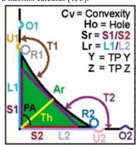
Welding joints are usually used in various buildings such as bridges or marine and submarine structures. It is well known that the geometry of the joint is important for realizing a fatigue computation. For some years, some Non-Destructive Controls Method have allowed us to get a quality control and obtain precise and discrete measurements of the geometry in order to make a fatigue calculus on the welded joints. A device named WISC based on a process of measurement by laser is used by DCNS to get a great number of trajectories of welded joints. Some geometrical parameters given in figure 1 can be measured with this device.

According with some studies, the parameters measured by the WISC are sufficient if we want to make a fiabilist calculus [1, 3].

Figure 1: Description of outputs of the WISC

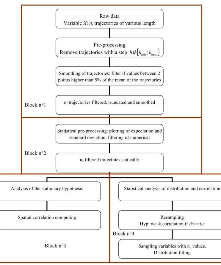
The study driven in this paper is a statistical analysis of one of the parameters. We give figure 2 the organigram which describes the different blocks and steps of the statistical analysis. Only the height of the joint S1 is studied in this paper. In the first two blocks, we only keep the most relevant measures by removing aberrant measurements. In the third block, we validate the stationary hypothesis of the second order. We also look for a length for which a hypothesis of non-correlation can be assumed. This distance can then be used in the last part of the work. It is useful to build some greater data to search the best probability law to represent the data distribution.

2 STATISTICAL PROCESSING METHOD

For the given data analysis, a statistical treatment is used, this methodology is detailed in figure 2.

Figure 2: Organigram of the used statistical analysis

We note X the variable studied here, nt the number

of trajectories initially given, nf the number of

trajectories after the data pre-processing, ns the

number of trajectories after the statistical pre-processing and ne the number of trajectories used

for the distribution analysis. The step between two

measures is noted h. The abscissa is noted x and θ is the event. X(x,θ) is therefore the random one-dimensional variable depending of the event and the abscissa. The usable measured length is noted

Ls. The number of measurements done on length Ls is denoted N. The following equations define

Raw data

Variable X: nt trajectories of various length

Pre-processing

Remove trajectories with a step h_∉

[

h_min; h_max

]

Smoothing of trajectories: filter if values between 2 points higher than 5% of the mean of the trajectories

nf trajectories filtered, truncated and smoothed

Statistical pre-processing: plotting of expectation and standard deviation, filtering of numerical

anomalies

ns filtered trajectoies statically

Analysis of the stationary hypothesis

Spatial correlation computing

Statistical analysis of distribution and correlation

Resampling

Hyp: weak correlation if Δx>>Lc

Sampling variables with ne values. Distribution fitting

Block n°1

Block n°2

Block n°3

different notations and discrete definitions of mean, standard deviation correlation coefficient used in this paper.

• The spatial mean of a particular trajectory i is given by:

( )

_∑

=

(

)

= = N j j i j i X X x N m 1 ; 1 θ θ (1) • The spatial standard deviation of the

trajectory i is given by:

( )

_∑

=

(

(

)

( )

)

= − = N j j i X i j i X X x m N s 1 2 ; 1 θ θ θ (2) • The mean of the trajectories at a particular

abscissa xj is given by:

( )

_∑

=

(

)

= = S n i i i j S j X X x n x 1 ; 1 θ µ (3) • The standard deviation of the trajectories is

given by:

( )

_∑

=

(

(

)

( )

)

= − = S n i i j X i j S j X X x x n x 1 2 ; 1 µ θ σ (4) In the paper, we also use notations µX and σX

without precising the abscissa. In this case, these are the spatial means of µX(x) and σX(x).

In the following, the term “expectation” will be used to designate the expectation of a probabilistic law.

We also need to define the correlation coefficient

ρX;Y of two particular vectors

( )

(

(

i

)

)

i _{ nS_} x X x X ;...; 1 ; _∈ = θ and

(

)

(

(

i

)

)

i _{ nS_} x x Y x x Y ;...; 1 ; _∈ Δ + = Δ + θ as :

(

)

(

)

( )

(

) (

(

)

(

)

)

( ) (

x x x

)

x x x x Y x x X n x x x Y X n i i Y i X i S Y X S Δ + Δ + − Δ + − = Δ +

∑

= = σ σ µ θ µ θ ρ 1 ; ; ; 1 ; (5) From this equation, we can compute 2 different kinds of correlations. The first one is the spatial correlation. It corresponds to the mean of the different values obtained for different abscissa xj

and using X=Y. We finally have:

( )

_∑

+

(

)

− = = Δ Δ Δ + + − = Δ 1 1 ; ; 1 1 k N Nx k k k X X x X x x x N N x _ρ ρ (6) where NΔx is the number of measurements on

length Δx.

The second correlation coefficient is the coefficient between 2 variables at a given abscissa. It is given by

( )

x

(

x x

)

Y X Y X; ρ ; ; ψ = (7) The process can be divided into 4 blocks (figure 2). In the first one, the data of the chosen variable

X are filtered. The mean step h between two points

of measurement is estimated. To start with, we have nt trajectories of various lengths. The

trajectories are removed under 2 conditions: • The ones where the step is too variable

along the trajectories ;

• The ones where h is too different of the mean step.

In order to simplify the treatment, the studies will be done using the number of points of measurement. The knowledge of this number and the mean step give us immediately the length Ls in

meters. The following process is the smoothing of the trajectories by overwriting the aberrant measures. We finally obtain nf trajectories filtered,

smoothed and truncated at a length Lf. This length

is the shortest of the nf trajectories.

In the second block, some trajectories can also be removed if there are some irregularities in the evolutions of the mean and the standard deviation. We plot the evolution of the mean

( )

x

X

µ

(equation (3)) and the standard deviation

( )

x

X

σ

(equation (4)) from nf trajectories. We finally

obtain ns trajectories of length Ls.

In the third block, we analyze the one-dimensional field X

(

x;

θ

)

_{where X is the analyzed parameter, x}

is the abscissa and θ is the event and we try to answer to the following questions:

• Is it a second order stationary?

• Does it have a length named “correlation length” denoted Lc for which the measures

are independent?

In the fourth block, we now consider ne

trajectories that correspond to the addition of the

ns previously considered and some other

trajectories that had been removed because they were too short. If a correlation length Lc exists, we

can build some new distribution by merging the values of the variable X at the abscissa x with the values at the abscissa x+Lc. We then look for the

most adapted probabilistic law to represent the obtained distribution. The choice of this law is made among the Gamma law, the normal law and the log-normal law by calculating and using the maximum likelihood.

3 RESULTS ON THE CORRELATIONS AND DISTRIBUTION

3.1 PRE-PROCESSING OF THE DATABASE We initially have nt=50 trajectories. Each of them

has a step of measurement hi and a length which

are all different.

During the first step of the pre-processing of data, we only keep the trajectories which have a step of measurement near the mean value h in order to avoid a re-sampling process for the purpose of spatial study.

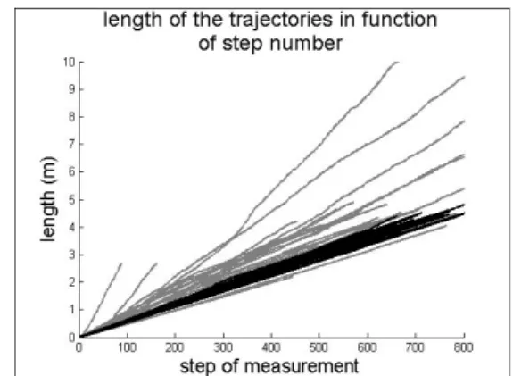
We plot the length of the trajectories as a function of the step number of measurement on the figure 3.

Figure 3: Plotting of the length of the trajectories in function of step number of measurement

Many trajectories plotted have a mean step of measurement nearly equal to the mean step h. To decide which trajectories will be kept, we estimate the mean step of each trajectory. First, we observe two of them with a mean step too different of the others and few measures. Those two trajectories are removed before all analysis.

Only the trajectories with a mean step h near 6mm are kept. We finally obtain ns=nf=22 trajectories

with a mean step h=6,2mm with a mean coefficient of variation equal to 41.4%. The analysis will be done on a length of Ls=3.62m.

3.2 ANALYSIS OF THE CORRELATION BETWEEN PARAMETERS

Before beginning the analysis of the random fields, we first verify if the physical coherence of the given database. To this purpose, a study on the correlation between fields is made (equation (7)). Preliminary to this study, we first assess the correlation for two different cases: a first one between fields that are presumably correlated and

a second between fields that are not correlated. Doing so, it will provide us an estimation of the correlation value for which we can assume that fields are not correlated.

The first case is that of known high correlation. We analyze the correlation between the area of the welded joint Area and the product between the height and the width of the joint S1*S2 and denoted ψArea_,S_1*S₂. The second one is the case of

low correlation between the overlap O1 and the height of the joint S1 and denoted ψO_{1 S, 1}. The

evolutions are given in figure 4 and 5.

We can observe a high correlation (over 0.9) and a weak noise for the correlation coefficient

2 * 1 ,S S Area

ψ in figure 4, which is in accordance with a functional relationship between the fields.

Figure 4: Analysis of the case of high correlation

On the contrary, we can observe a low mean value of the correlation (over -0.1) between the height of the joints and the overlap. This could be due to the great noise or to the hardness of measurement of one of these parameters (O1 in our example).

Figure 5 : Analysis of the case of low correlation

3.3 ANALYSIS OF THE CORRELATIONS Once we have limited the length of measurement, kept only the most homogeneous trajectories and verified the coherence of the database, we can analyze the trajectories retained.

This part of the analysis corresponds to the third block of the organigram (figure 2). We try to see if the hypothesis of the stationary of the second order is verified. We also search if a correlation length

Lc exists, distance that could be used to build some

new samples with values with low correlation (following Bravais-Pearson). These values could therefore be considered as independent.

In order to validate the stationary hypothesis, some equalities given below have to be verified:

( )

( )

(

x x

)

(

x x

)

x x x x X X X X X X X − = = = ∀ ' ' , , , , ' , ; ρ ρ σ σ µ µ (8)

We plot in figures 6 and 7 the different evolutions of mean, standard deviation and correlation coefficient with the length.

Figure 6: Analysis of mean and standard deviation of the field S1

We can observe that the values of mean and standard deviation are constant with respect to the abscissa x. Indeed, we can note 15.00

1 =

S

µ and

its coefficient of variation with respect to x is only 1.1%. Concerning the standard deviation, the mean value is 0.78

1 =

S

σ with a coefficient of variation of 16%. Having only ns=22 trajectories

for the analysis, we can consider that the standard deviation is also constant with the abscissa.

Now, we decide to analyze the spatial correlation coefficient (equation (6)). We obtain the presented curve on figure 7. The bold curve corresponds to the evolution of the mean of the coefficient, the two thinner curves around the bold one correspond to the coefficient with more or less one standard deviation.

Figure 7: Spatial correlation coefficient of S1

The coefficient is decreasing until a length equal to 1.5m. This evolution helps us conclude that the stationary hypothesis of the second order can be validated. Nevertheless, after the decrease of the

increase of the coefficient is observed. This latter phenomenum is not explained in this paper, but some complementary studies are currently in advancement.

To determine the distance Lc for which the values

of X are non-correlated, we first have to estimate the threshold value of correlation for which the hypothesis of uncorrelation is valid. As mentioned in section 3.2, we choose two physically non-correlated variables. In this case, we consider the variables S1 and O1 previously presented and we give the repartition of the value of the correlation between these two variables ψS_{1 O, 1} in figure 8.

Although the correlation should be equal to 0 in theory, in practice the deviation with this theoretical value is important.

Figure 8: Distribution and apprach with a normal law of the repartition of the correlation between O1 and S1

By approaching this distribution with a normal law with the maximum likelihood estimator, the parameters of the law are E=0.13 for the expectation and σ=0.22 for the standard deviation. Considering the confidence interval at 95% (

[

_E−2

σ

;_E+2

σ

]

for a normal law), the interval of non-correlation is over

[

−0.5;0.3

]

. Finally non correlation is assumed for _ρ

( )

_{Δx ≤}0.3_{. Looking} at figure 7, we can therefore consider a correlation distance Lc=1.5m.

Once having validated the second order stationary hypothesis and determined the length Lc for which

the hypothesis of non-correlation between values is acceptable, we can identify a probabilistic law to represent the distributions using the maximum likelihood.

The length of measurement Ls being much longer

than the correlation length Lc, we can merge 22

values at abscissas x=0.46m, x=1.96m and

x=3.46m thus providing 66 samples. The

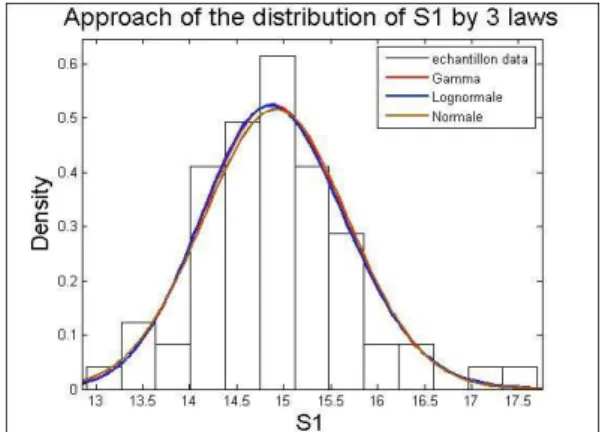
corresponding distribution of S1 is depicted in figure 9.

Figure 9: plotting of three chosen laws on the distribution of S1

As told earlier in section 2, we identify three different laws, the Gamma law, the normal law and the log-normal law. The corresponding values of expectation, standard deviation and maximum of likelihood are summarized in table 1.

E σ Maximum likelihood Gamma 14.92 0.76 -75.61 Normal 14.92 0.77 -75.38 Log-normal 14.92 0.77 -76.17

Table 1: Values of expectation, standard deviation and maximum likelihood for each law

Although the values of maximum of likelihood are similar, we retain the log-normal law as the best of the three laws to approach the distribution given by the 66 values of S1. This choice is only based on the value of maximum log-likelihood and allows only positive values of the geometrical parameter S1.

4 CONCLUSION

The measurement of the geometry of welded joints is made easier thanks to devices using laser process. In particular, the device WISC is used for the measurement in this article. Some errors in the measurement or some experimental difficulties are present in the given data. These problems come in addition of the randomness on the geometrical parameters that appear during the welding process. In this paper, we have to use statistical processing method using different steps to achieve the analysis. But, for this purpose, we can only use less of the half of the given database. This hypothesis allows us to increase the number of samples by re-sampling using the correlation length.

AKNOWLEDMENTS

Authors wish to thank Direction Générale de l’Armement for financing these works by the Programme d’Etudes Amont COMENAV (market n°2007 90 0907)

REFERENCES

1. [Huther I.], [1996] ‘[Prévision du comportement à la fatigue des assemblages soudés – prise en compte de l’effet macro, micro-géométrique]’, [Mémoire de thèse de l’Université Blaise

Pascal (Clermont-Ferrand 2), soutenue le 11 juin 1996 à Clermont-Ferrand]

2. [Vanmarcke E.], [1983] ‘[Random fields, analysis and synthesis]’, [The MIT Press

3. [Schoefs F., Chevreuil M., Clément A., Cazuguel M., Pasqualini O.], [2010] ‘[Reliability of marine welded joints subjected to stochastic geometry : from measure to computation]’, [Proceeding of

5th Conference on Network for Integrating Structural Analysis, Risk and Reliability, 7 pages, 14-16 June 2010, Edinburgh, Scotland, UK]

4. [Pasqualini O., Schoefs F., Chevreuil M., Cazuguel M.], [2011] ‘[Analyse de la variabilité spatiale géométrique pour la fiabilité des cordons de soudure]’, [20ème

Congrès Français de Mécanique – Incertitudes, Fiabilité et Maîtrise des Risques, 5 pages, 28 Août au 2 Septembre