HAL Id: hal-01164751
https://hal.archives-ouvertes.fr/hal-01164751
Submitted on 17 Jun 2015
HAL is a multi-disciplinary open access
archive for the deposit and dissemination of
sci-entific research documents, whether they are
pub-lished or not. The documents may come from
teaching and research institutions in France or
abroad, or from public or private research centers.
L’archive ouverte pluridisciplinaire HAL, est
destinée au dépôt et à la diffusion de documents
scientifiques de niveau recherche, publiés ou non,
émanant des établissements d’enseignement et de
recherche français ou étrangers, des laboratoires
publics ou privés.
Boolean Network Identification from Multiplex Time
Series Data
Max Ostrowski, Loïc Paulevé, Torsten Schaub, Anne Siegel, Carito
Guziolowski
To cite this version:
Max Ostrowski, Loïc Paulevé, Torsten Schaub, Anne Siegel, Carito Guziolowski. Boolean Network
Identification from Multiplex Time Series Data. CMSB 2015 - 13th conference on Computational
Methods for Systems Biology, Sep 2015, Nantes, France. pp.170-181, �10.1007/978-3-319-23401-4_15�.
�hal-01164751�
Boolean Network Identification from Multiplex
Time Series Data
M. Ostrowski1?, L. Paulev´e2?, T. Schaub1, A. Siegel3,, C. Guziolowski4 1
Potsdam University, Computer Science Department, Postdam, Germany.
2 CNRS, Universit´e Paris-Sud LRI-UMR 8623, Orsay, France 3
CNRS, Universit´e de Rennes 1, IRISA-UMR 6074, Rennes, France
4 Ecole Centrale de Nantes, IRCCyN UMR CNRS 6597, Nantes, France.´
Abstract. Boolean networks (and more general logic models) are use-ful frameworks to study signal transduction across multiple pathways. Logical models can be learned from a prior knowledge network structure and multiplex phosphoproteomics data. However, most efficient and scal-able training methods focus on the comparison of two time-points and assume that the system has reached an early steady state. In this paper, we generalize such a learning procedure to take into account the time series traces of phosphoproteomics data in order to discriminate Boolean networks according to their transient dynamics. To that goal, we exhibit a necessary condition that must be satisfied by a Boolean network dy-namics to be consistent with a discretized time series trace. Based on this condition, we use a declarative programming approach (Answer Set Programming) to compute an over-approximation of the set of Boolean networks which fit best with experimental data. Combined with model-checking approaches, we end up with a global learning algorithm and compare it to learning approaches based on static data.
1
Introduction
Generic prior knowledge about canonical cell signaling networks can be retrieved from database sources. They provide a first insight on how cells respond to their environment by triggering processes such as growth, survival, apoptosis (cell death), and migration. However, little is known about the exact chaining and composition of signaling events within these networks in specific cells and specific conditions, as provided by the simulations of predictive mathematical models (e.g. a set of differential equations or a set of logic rules). When building predictive models, the parameters of a model (built accordingly to generic prior knowledge) can be fitted to the data to obtain the most plausible model for a specific cell type, if enough experimental data is available. This is normally achieved by defining an objective fitness function to be optimized. In this context, post-translational modifications, notably protein phosphorylation, play a key role in signaling. They are very useful for the training of model parameters
?
through the use of multiplex phosphorylation assays, a recent form of high-throughput data providing information about protein-activity modifications in a specific cell type upon various perturbations (clamping) [1].
Boolean logical networks [12] provide a simple yet powerful qualitative frame-work which has become very popular during the last decade to model signaling or regulatory networks [16]. In contrast to quantitative methods which permit fine-grained kinetic analysis, qualitative approaches allow for addressing large-scale biological networks. In this context, the manual identification of logic rules underlying the system has been addressed under different hypotheses and meth-ods [4]. Although, scalable methmeth-ods restrain themselves to learning models from two time points (start; end), assuming the system has reached an early steady-state when the measurements are performed. As shown in [14], this assumption prevents capturing important characteristics of signaling networks such as loops. The goal of this paper is to introduce a new method to infer Boolean net-works (BNs) from time series datasets which scales to the size of currently studied BNs. Given multiplex time series data from the measurement of a partial set of biological entities under different experimental conditions, we want to identify all the BNs that have a structure compatible with a given prior knowledge in-teraction graph and that can reproduce all the (experimentally) observed time series. Time series data are assumed incomplete, i.e., only a subset of network components are observed, with measurements made at discrete time points and with normalized continuous values. It is possible that no BN, constrained by the prior interaction graph, reproduces all the input time series. In such a case we introduce a fitness function to measure the distance between a trace of a BN simulation and a measured time series. Therefore, we aim to infer the BNs whose dynamics contains traces with the best fitness to all measurements.
Our approach relies on the combination of several techniques. First, we intro-duce a necessary condition for a discretized time series data to be the trace of a BN. This provides an over-approximation of the successive reachability proper-ties, leading to reject BNs that cannot reproduce the time series without a costly exhaustive analysis of the dynamics. Then, we use efficient declarative program-ming approaches (Answer Set Programprogram-ming; ASP) to enumerate BNs which approximate the best experimental data while satisfying the necessary condition on the dynamics. At the end, we obtain a set of BNs associated with traces which both satisfy the necessary condition and optimally fit with experimental data. Because of the reachability over-approximation, part of the returned BNs cannot reproduce the associated Boolean traces. Such false positives can be detected a posteriori using a model-checking approach on the returned results.
We evaluated our inference method on synthetic data generated from BNs between 13 and 17 nodes. On those BNs, six nodes have been selected as observ-able, and several experimental conditions have been simulated. Our prototype implementation has been able to identify efficiently all BNs satisfying the neces-sary condition with a very low rate of false positives. Finally, we estimated the added-value of models identified with our method on the full time series with models learned from two time points, considered as a steady state.
2
Boolean Network Identification
2.1 Admissible Boolean Networks and multiplex time series data Boolean Networks (BNs). A BN with n components {1, . . . , n} consists of a tuple of n functions F = (f1, . . . , fn) where each function fi : Bn → B, B
∆
= {0, 1}, i ∈ {1, . . . , n}, associates to each global state x ∈ Bnof the network with the next
value of the i-th component. The value of the i-th component in x is noted xi.
The transitions between global states of the network are specified with a reflexive transition relation → ⊆ Bn× Bn. The transitive closure of → is denoted by →∗.
Given x, x0∈ Bn, x →∗x0 if and only if, either x = x0, or x → · · · → x0.
Concrete semantics for the transition relation. Several definitions of the tran-sition relation → can be used depending on the update schedule of the compo-nents [2], ranging from so-called parallel (or synchronous) updates where each transition updates the value of all the components, to the asynchronous update where each transition updates the value of only one component chosen non-deterministically. As the over-approximation results presented in this article are independent from the update schedule, we use the general definition, where any number of components can be updated during a transition: for any x, x0∈ Bn,
x → x0 ∆⇔ ∀i ∈ {1, . . . , n}, x0i6= xi⇒ x0i= fi(x) . (1)
Prior Knowledge Network and admissible BNs. An interaction graph between n components is a digraph between nodes {1, . . . , n} where each edge is signed, i.e., either positive or negative. The interaction graph of a BN F , noted IG(F ), has a positive (resp. negative) edge from node j to node i if and only if there exists x, x0∈ Bn which are identical except on the j-th coordinate where x
j = 0
and x0j= 1 and such that fi(x) < fi(x0) (resp. fi(x) > fi(x0)).
In the rest of the paper, the Prior Knowledge Network (PKN) is an interac-tion graph which delimits the set of admissible BNs: a BN F is admissible with respect to a PKN G if and only if IG(F ) is a sub-graph of G and IG(F ) has at one most (signed) edge between two nodes.
Multiplex Time Series Data. We consider classical biology experimental set-tings where the activity of a subset of biological species is observed over time, at discrete time points, in different experimental conditions, ranging over var-ious input signals and clamping operations. Clampings consist of a subset A of components with a forced activation, and a subset I of components with a forced inhibition. Given a BN F = (f1, . . . , fn), the corresponding clamped BN
F[A,I]= (f10, . . . , fn0) is defined for all i ∈ {1, . . . , n} as:
fi0 =∆ x 7→ 1 if i ∈ A x 7→ 0 if i ∈ I fi otherwise.
Without loss of generality, we assume that the time series data relate to the observation of m ≤ n nodes that match the nodes {1, . . . , m} of the BN (so the nodes {m + 1, . . . , n} are not observed). The observations consist of normalized continuous values: a time series of k data points is denoted by T = (t1, . . . , tk),
with ∀j ∈ {1, . . . , k}, tj∈ [0; 1]m.
Hereafter, we consider a simple binarization of observations using a 0.5 threshold: given a continuous observation tji ∈ [0; 1] of a component, its Boolean value is noted η(tji) where η(tji)= 1 when t∆ ji ≥ 0.5, and η(tji)∆= 0 otherwise. The distance between a binary sequence X = (x1, . . . , xk), where ∀i ∈ {1, . . . , k}, xi∈
Bm, and a time series T is evaluated with the standard Mean Squared Error : mse(X, T )=∆ q Pk j=1 Pm i=1(x j i − t j i) 2 .
2.2 Over-approximation of Boolean network verification
Given a BN F and a pair of states x, y ∈ Bn, checking the reachability of y
from x (x →∗ y) is a standard model-checking task, known to have a limited scalability due to its theoretical complexity (NP-complete [11]). In this section, we introduce a so-called meta-state semantics (⇒) for BNs. From such seman-tics, we express a necessary condition for reachability in the concrete semantics (→), referred to as support consistency ( ∗). Meta-state semantics offers prop-erties (notably monotonicity) that make support consistency efficient to verify, in particular with ASP. However, support consistency is not a sufficient condi-tion for reachability, so this approach may lead to false positives but guarantees the absence of false negatives. Therefore, we will apply exact model-checking approaches on the inferred BNs in order to rule out false positives. Thanks to the over-approximation criteria, one can expect that the set of BNs satisfying the necessary condition is small compared to the full domain of BNs delimited by the PKN, leading to a global gain in terms of performance.
Meta-state semantics. A meta-state u of dimension n is a vector of n non-empty subsets of B, noted M∆= {{0}, {1}, {0, 1}}; the set of meta-states is Mn. In the following, meta-states characterize a set of Boolean states: a state x ∈ Bnbelongs
to a meta-state u ∈ Mn, noted x ∈ u, iff each Boolean component x
i belongs to
the set ui, i.e., ∀i ∈ {1, . . . , n}, xi∈ ui. Given a state x ∈ Bn, x is the meta-state
such that ∀i ∈ {1, . . . , n}, xi = {xi}. In the scope of a BN F = (f1, . . . , fn),
we define a reflexive transition relation between meta-states ⇒ ⊆ Mn× Mn as
follows: from a meta-state u, there is one transition for each i ∈ {1, . . . , n} which adds to ui all the possible values of the function fi applied to every x ∈ u:
u ⇒ v⇔ ∃i ∈ {1, . . . , n}, v = hu∆ 1, . . . , ui∪ {fi(x) | x ∈ u}, . . . uni . (2)
Several properties arise from this definition, in particular u ⇒ v implies that ∀i ∈ {1, . . . , n}, ui ⊆ vi; therefore x ∈ u ⇒ x ∈ v (monotonicity). Moreover,
Lemma 1 establishes the consistency of the meta-semantics (⇒) with the con-crete semantics (→): given x, y ∈ Bn, x → y requires that there exists a
meta-state u such that y ∈ u and x ⇒∗ u, where ⇒∗ is the transitive closure of ⇒.
Lemma 1. ∀x, y ∈ Bn, x → y =⇒ ∃u ∈ Mn, y ∈ u : x ⇒∗u.
Proof. Assuming x → y, let us define the set I = {i ∈ {1, . . . , n} | y∆ i 6= xi}.
From equation (1), ∀i ∈ I, yi= fi(x). Let us assume that for some strict subset
J ( I, ∃v ∈ Mn
, x ⇒∗ v with ∀i ∈ J , yi∈ vi. It is notably the case with J = ∅.
By induction, we show that, for any k ∈ I \ J , ∃u ∈ Mn
such that x ⇒∗ v ⇒ u with ∀i ∈ J ∪ {k}, yi ∈ ui. Remarking that x ∈ v and defining u ∈ Mn such as
ui = vk∪ {fk(z) | z ∈ v} if i = k and ui = vi if i 6= k, we obtain that v ⇒ u,
with yk= fk(x) ∈ uk. ut
Such a necessary condition for reachability can be furthermore refined by ensuring that for each component i ∈ {1, . . . , n} that is equal in x and y, if all meta-states u containing y with x ⇒∗u are such that ui= {0, 1}, then u contains
a state z with fi(z) = yi = xi. Intuitively, this refinement ensures that if the
i-th component has to temporarily change its value for reaching y, a state from which it can recover its initial (and final) value has to be reached in between. Such a condition is referred to as support consistency (definition 1). Theorem 1 states that support consistency is a necessary condition for reachability. Definition 1 (Support Consistency ( ∗)). A state x ∈ Bn is
support-consistent with y ∈ Bn
, denoted by x ∗ y, if and only if there exists u ∈ Mn
with x ⇒∗ u such that y ∈ u and for all i ∈ {1, . . . , n} where yi = xi, ui =
{0, 1} =⇒ ∃z ∈ u : fi(z) = yi.
Theorem 1. ∀x, y ∈ Bn, x →∗
y =⇒ x ∗y.
Proof. Let us consider any tuple of states (x1, . . . , xk) with x1= x, xk= y, and ∀j ∈ {1, . . . , k − 1}, xj → xj+1
. From lemma 1, ∃u ∈ Mn
such that x ⇒∗u and
∀j ∈ {1, . . . , k}, xk ∈ u. If for all such u, for any i ∈ {1, . . . , n}, u
i = {0, 1}
implies that there exists l ∈ {1, . . . , k} with xl
i6= xi. If yi= xi, there necessarily
exists m ∈ {l, . . . , k − 1} such that fi(xm) = yi. Therefore xm∈ u. ut
2.3 Optimization with respect to time series data
Our objective is to infer BNs that are admissible with a given PKN and that verify the sequential reachability of binary states in Bm that are as close as possible to a given time series data and its associated experimental settings. Distance between a time series data and a BN. Given a time series T with associated clamping A, I, the distance between a BN F and (T, A, I), noted mse(F[A,I], T ), is the minimal MSE between T and a sequence of binary states
in F[A,I]: x1 →∗ x2. . . →∗ xk. We notice that the lowest possible mse(X, T )
among all Boolean traces is the MSE between T and its binarization η(T ) = ((η(t1i))i=1...m, · · · , (η(tki))i=1...m). Let us call MSET
∆
= mse(η(T ), T ) this min-imum MSE which is intrinsic to the time series T and to the threshold for binarization (0.5); mse(F[A,I], T ) ≥ MSET. Whenever mse(F[A,I], T ) = MSET,
we say the BN F reproduces the time series data T .
Relaxing the semantics constraint. In order to prevent an exhaustive exploration of the BN dynamics for characterizing the sequences of reachable (→∗) Boolean states, we consider any sequence X = (x1, . . . , xk), with ∀j ∈ {1, . . . , k}, xj ∈ Bn,
that are support-consistent ( ∗), i.e., x1 ∗ x2
. . . ∗ xk in the scope of the
BN F[A,I]. The MSE of such a support-consistent Boolean state sequence X
w.r.t. the time series T is noted mse(X, T ); and the minimal distance amongd all support-consistent sequences in F[A,I]with T is referred to asmse(Fd [A,I], T ). Because any reachable sequence is support-consistent (theorem 1), we obtain that mse(F[A,I], T ) ≥mse(Fd [A,I], T ) ≥ MSET; and in particular mse(F[A,I], T ) 6= d
mse(F[A,I], T ) only if none of the support-consistent sequences X with minimal
d
mse(X, T ) are actually sequences of reachable Boolean states. In such cases, F is a false positive. Determining if F is a true positive can be done a posteriori with a model-checking approach: ifmse(Fd [A,I], T ) = MSET, we check that η(T )
is a valid sequence of reachable states in F[A,I]; otherwise, we check the validity
with respect to reachability of at least one sequence X with minimalmse(X, T ).d Optimization problem. We consider a PKN G and a set of r multiplex time series D = (T1, A1, I1), . . . , (Tr, Ar, Ir). The distance between a BN F and
the dataset is the sum of distances mse(F, D)d ∆= Pr
l=1mse(Fd [Al,Il], T
l). The
optimization procedure identifies the BNs compatible with the PKN G that have the minimal distancemse(F, D). In the scope of this paper, we enforce that eachd non-observed node starts with the same initial value in all the time series: for each l ∈ {1, . . . , r}, if Xlis a sequence of support-consistent Boolean states in Bn such thatmse(Fd [Al,Il], Tl) = mse(Xl, Tl), for all i ∈ {m + 1, . . . , n}, X1,il = X1,i1 .
Whereas this constraint reduces the space of sequences to explore, it also ensures consistency between the different experimental settings.
Depending on the number of nodes in the PKN, and on the discriminative power of the time series dataset, a rather large number of BNs may be expected to be inferred. As an alternative, we can output only the BNs having the smallest Disjunctive Normal Form (DNF) representation with respect to clause inclusion, i.e., no literal nor clause can be removed. This means that no unnecessary edges occur in the BNs, thus providing only the simplest BNs. In the following, we refer to such a set of solutions as subset-minimal.
2.4 Implementation
Answer Set Programming (ASP; [3,7]) is a declarative approach to solving knowl-edge-intense combinatorial (optimization) problems comprising up to tens of
millions of variables. ASP’s distinguishing combination of a high-level model-ing language with high-performant solvmodel-ing tools allows for concentratmodel-ing on an actual problem, rather than a smart way of implementing it. The basic idea of ASP is to express a problem in a logical format so that the (logical) models of its representation provide the solutions to the original problem. Problems are expressed as logic programs and the resulting models are referred to as answer sets. Although determining whether a program has an answer set is the fun-damental decision problem in ASP, modern ASP solvers like clasp [9] support various combinations of reasoning modes, among them, regular and projective enumeration, intersection and union, multi-criteria optimization and subsets [8] and/or sum-based minimal (maximal, resp.) model enumeration.
Here we describe the general design of the encoding, while the complete ver-sion is available online5. For the encoding we follow the general design approach in ASP in a way that we first guess all admissible BNs given a PKN. Guessing in this context does not mean choosing a BN by some heuristic, but exhaus-tively trying all possible combinations of edges and logical connectives. We also guess time series, a value {0, 1} for every species in every experiment and every time point. In the case of non-observed nodes we add a constraint that fixes their initial value, at time point 0, across all the experiments. We then restrict this search space by posting constraints that the guessed time series shall be support-consistent with the guessed BN. In this way all enumerated BNs are consistent with the guessed time series. As an optimization function we mini-mize the distance between the guessed time series and the measured one. In the optimal case, this means that the guessed time series is equal to the measured one, and the BN is support-consistent with the measured data.
3
Evaluation
3.1 Case study
As a proof of concept we used the PKN published in [14] (see the compressed PKN in Fig. 1A). From this PKN, the authors of [14] randomly generated an admissible golden-standard BN to simulate synthetic time series data (Fig. 1C). Afterwards, they removed the link from tnfa to ap1 from the PKN to represent incomplete regulatory knowledge. After confronting the incomplete PKN with the time series data, our method learned a family of BNs consisting of 3 subset-minimal BNs. All BNs were checked to be true positives, therefore they have an optimal MSE score of 0.07 with respect to the data. The family of optimal BNs was learned after 0.04 seconds of computation on a standard desktop computer. In Fig. 1B we plot the subset-minimal family of BNs learned for this case study. It recovers the complete logical behaviors of the golden-standard, except for the one regulation from tnfa to ap1 which was removed from the PKN. Only the logical function of the regulation over p38 is not consensually learned across all BNs in the family; the rest of logical functions learned are shared by all models. The quality of our results concerning the learned BNs is comparable to the one obtained in [14] for the same case study. The computation time of our method
Fig. 1. (A) Compressed PKN from [14]. Green and red edges indicate activations and inhibi-tions respectively. Colors of the nodes represent the chosen experimental design: green refers to inputs/stimuli, red, to inhibited nodes, and blue, to measured species. (B) Boolean networks (BNs) learned from time series data which are subset-minimal. All BNs predictions have minimal ∆MSE with respect to the synthetic time series data. A black circle represents a logical AND gate. A number written over an edge represents the frequency of this logical gate or edge with respect to the family of BNs when the edge is not shared by all BNs. (C) Synthetic time series data used in [14] simulated using a BN admissible for the PKN in A. In total 10 experimental conditions were simulated. Red boxes indicate the minimal set of 3 error time-points detected.
improves the one of published methods in a range of 2 to 4 orders of magnitude. Moreover, our method is exhaustive: all logical networks are learned. The full set of solutions (not only the subset-minimal BNs) was also computed showing one more BN with an OR gate above p38 from tnfa and map3k1.
The method also automatically identified the list of minimal errors in the time series data, selecting time-points that cannot be explained by the learned BNs. For the case of all optimal BNs, we found the following 3 errors (see Fig. 1C) in all of them. For experiment 10, time-point 10, species p38, the error can be explained by the noise artificially introduced in the dataset. The predecessors of p38 are tnfa and egfr, both active in experimental condition 10 (see Fig.1C). The signal of p38 can therefore only increase (or stay the same). However, the measure of p38 slightly decreases (due to noise) at time-point 10; this generates an error since the BNs cannot satisfy the data at this particular time-point. For experiment 6, time-point 2 and 4, species ap1, the errors can be explained by the fact that one edge (the link from tnfa to ap1) was deleted from the PKN, but was kept to generate the synthetic time series data. All BNs agree on a regulation of p38 and ap1 from map3k1. In experiment 6 tnfa is stimulated and pi3k is inhibited (see Fig. 1C). At time-point 2 the value of map3k1 has to be activated (transition 0 → 1) to justify the activation of ap1. However, since map3k1 is the only regulator of p38, which is all the experiment at value 0, this cannot be explained by the BN and generates an error.
3.2 Benchmarks
In this section we evaluate our method for BN identification on synthetic mul-tiplex time series data. Given a PKN, a dataset and a set of inferred BNs, we focus on two evaluation criteria: the MSE distance of the BNs to the dataset, and the rate of false positives due to our reachability over-approximation.
Synthetic multiplex time series datasets. 10 PKNs were derived by randomly removing or adding edges from the compressed PKN published in [14]. For each PKN we randomly selected 3 standard admissible BNs. Each golden-standard BN was used to generate synthetic time series data by simulating the BN with logic-based ODEs. In total we generated 30 datasets (see appendix A for details).
MSE computation. Following section 2.3, our method optimizes the MSE of the BNs F to the dataset D up to the reachability over-approximation criteria: if the BN is a true positive, the estimated MSEmse(F, D) is the exact MSE mse(F, D),d otherwise the estimated MSE is an under-approximation - the exact MSE may be larger. Due to the optimization, all the BNs have the same estimated MSE. The value of the estimated MSE can be computed using the equation given in section 2.1 by sampling one BN from the result set with one Boolean trace X for each time series T of dataset D such thatmse(X, T ) is minimal.d
True-positive rate computation. Any BN inferred by our method satisfies the necessary condition depicted in section 2.2 for producing Boolean traces as close as possible to a given time series dataset. Verifying that the BN can actually reproduce those Boolean traces requires an exhaustive analysis of the dynamics to ensure the successive reachability of the Boolean states. In the scope of this paper, we performed such a verification using a model-checking approach. The presented experiments have been conducted using the tool NuSMV [5] which allows an efficient encoding of the dynamics accounting for the range of clamping settings of the different time series in the dataset5. The true-positive rate
eval-uation proceeds by iteratively checking each inferred BN. In the case when the estimated MSE is MSET (section 2.3), the model-checking is performed with
re-spect to the binarized time series. Otherwise, we iterate over the closest Boolean traces computed in section 2.3 until a sample is validated by model-checking; if no such a sample exists, the BN is a false positive.
Results. For each dataset, the model identification has been performed with respect to the PKNs from which the BNs used for data generation have been extracted; and with respect to the PKNs where some edges have been deleted so the BNs used to generate the data are not in the considered domain. Detailed results are given in appendix B. With the exact PKNs, the estimated MSE is always the minimum MSET; moreover, the rate of true positive is 100% in 28
benchmark datasets, and above 90% in the 2 others. With the PKNs with deleted edges, most of the cases show a very high true positive rate (often 100%) and an estimated MSE close to (often equal to) MSET. Note that for some dataset, no
true positive has been found. For the cases when the estimated MSE is different from MSET, the true positive rate can only be evaluated by sampling Boolean
traces close to the time series data. Because of the very high combinatorics of such sampling space, the computation has been aborted after one hour, hence
5
we cannot guarantee that no true positive exists. When no true positives have been identified, the MSE may be under-estimated.
The inference of the subset-minimal solutions for the 30 benchmarks with exact PKNs took less than 2 seconds on average. The performance is similar for the benchmarks with incomplete PKNs that contained a true positive BN in the result. The number of results varies between 12 and 2640 with the exact PKN and from 2 to 1188 with modified PKNs. Depending on the size and the complexity of its dynamics, the model-checking of one BN took between 1s and 5 minutes. The full set of solutions (not only the subset-minimal BNs) have also been performed with the exact PKN, showing very similar results and running time, with subsequently more results (up to 54,000 BNs, data not shown).
Same experiments have been conducted on the time series generated with noise (appendix A) but show no difference in the results (data not shown). This may indicate that the noise influence may be tempered by the binarization.
3.3 Comparison with inferences using pseudo steady-states
In this section we compare our results with the previously developed approach Caspo [10]. Caspo, as well as other state-of-the-art approaches such as CellNopt [15], considers two time-points (an initial point and a pseudo-steady state) and a PKN. It computes a set of BNs with minimal size that can explain the best the transition between the two time-points. Due to its static nature and the minimal size condition, it is not possible to infer feedback loops or dynamic behaviour, because models with loops would not improve the fitting with the data assuming a steady state. With this comparison, we aim at emphasizing the importance of taking into account model dynamics to obtain accurate model predictions.
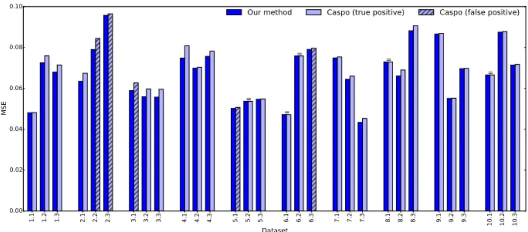
Applied on the 30 synthetic datasets of section 3.2 with the PKNs used for the data generation, we compared the best MSE obtained applying our optimization procedure on the BNs returned by Caspo on one time point (assumed steady by Caspo) and on all BNs delimited by the PKNs. Therefore, we compare the best estimated MSE with respect to the multiplex time series for both the Caspo approach and the method introduced by this paper. As explained in section 2.3, and as in section 3.2, the computed MSE may be under-estimated so we used model-checking a posteriori to verify the presence of true positive BNs.
Figure 2 plots the estimated MSEs, where the 6th time point of the time series has been selected for the learning with Caspo; other time points give very similar results (data not shown). On the contrary to our approach where it was always possible to find a BN which was fully consistent with the data, having the minimum M SE = MSET, Caspo failed to identify a consistent model
with the data in 25 over the 30 experiments. Among those 25 experiments, the estimated MSE on Caspo results may be under-estimated in 5 experiments where the returned BNs are actually false positives (streaked bars). This evidences the role of feedback loops which cannot be captured with a two-timepoints learning procedure and the information gain brought by time series data.
1.1 1.2 1.3 2.1 2.2 2.3 3.1 3.2 3.3 4.1 4.2 4.3 5.1 5.2 5.3 6.1 6.2 6.3 7.1 7.2 7.3 8.1 8.2 8.3 9.1 9.2 9.3 10.1 10.2 10.3 Dataset 0.00 0.02 0.04 0.06 0.08 0.10 MSE = = = = =
Our method Caspo (true positive) Caspo (false positive)
Fig. 2. Comparing MSE with Caspo for 10 different PKNs with 3 datasets each. “=” indicates equal MSE.
4
Conclusion
We have introduced a procedure based on combinatorial optimization with declar-ative programming approaches and model checking to identify BNs from multi-plex time series data given a prior network structure. To cope with the commulti-plex- complex-ity of an exhaustive analysis of BNs dynamics, we defined an abstract semantics of BNs from which we derived a necessary condition for the satisfaction of suc-cessive reachability properties, induced by the time series data. Our procedure identifies all the BNs that satisfy this necessary condition with the shortest distance (in terms of MSE) to the observed experimental data. Because the sat-isfaction criteria for the dynamics is over-approximated, our method may lead to BNs that are false positive, and have an under-estimated MSE. Applied to synthetic multiplex time series datasets on networks composed of 13 to 17 nodes, the identification of BNs takes only a few seconds and exhibits a very low rate of false positives, showing a remarkable efficiency.
In the present form, we assume that the experimental data is normalized be-tween 0 and 1 and use a discretization threshold at 0.5. Whereas such a setting is relevant for phosphoproteomics data, future work may generalize our opti-mization framework to account for adaptive and multiple discretization levels. Moreover, application to larger networks should be considered, although few of such data are currently available, and generating synthetic data with sufficient discriminant power may be challenging.
Because our identification method can be exhaustive, the framework we pro-pose is suited for the complete Thomas parameters identification for BNs from incomplete time series data [13,6].Thanks to our abstract semantics, our method is able to filter out very efficiently a large number of candidate BNs without a costly exact model-checking, which is postponed to the validation of the results. In that way, future work may further explore the combination of dynamics
over-approximations with model-checking approaches to provide scalable and exact inference of BNs from time series data.
References
1. L. G. Alexopoulos, J. Saez-Rodriguez, B. Cosgrove, D. A. Lauffenburger, and P. Sorger. Networks inferred from biochemical data reveal profound differences in toll-like receptor and inflammatory signaling between normal and transformed hepatocytes. Molecular & Cellular Proteomics, 9(9):1849–1865, 2010.
2. J. Aracena, E. Goles, A. Moreira, and L. Salinas. On the robustness of update schedules in boolean networks. Biosystems, 97(1):1 – 8, 2009.
3. C. Baral. Knowledge Representation, Reasoning and Declarative Problem Solving. Cambridge University Press, 2003.
4. N. Berestovsky and L. Nakhleh. An evaluation of methods for inferring boolean networks from time-series data. PLoS ONE, 8(6):e66031, 2013.
5. A. Cimatti, E. Clarke, E. Giunchiglia, F. Giunchiglia, M. Pistore, M. Roveri, R. Se-bastiani, and A. Tacchella. NuSMV 2: An opensource tool for symbolic model checking. In Computer Aided Verification, volume 2404 of LNCS, pages 241–268. Springer Berlin / Heidelberg, 2002.
6. E. Gallet, M. Manceny, P. Le Gall, and P. Ballarini. An ltl model checking approach for biological parameter inference. In Formal Methods and Software Engineering, volume 8829 of LNCS, pages 155–170. Springer, 2014.
7. M. Gebser, R. Kaminski, B. Kaufmann, and T. Schaub. Answer Set Solving in Practice. Synthesis Lectures on Artificial Intelligence and Machine Learning. Mor-gan and Claypool Publishers, 2012.
8. M. Gebser, B. Kaufmann, R. Otero, J. Romero, T. Schaub, and P. Wanko. Domain-specific heuristics in answer set programming. In Proceedings of the 27th National Conference on Artificial Intelligence (AAAI’13), pages 350–356. AAAI Press, 2013. 9. M. Gebser, B. Kaufmann, and T. Schaub. Multi-threaded ASP solving with clasp.
Theory and Practice of Logic Programming, 12(4-5):525–545, 2012.
10. C. Guziolowski, S. Videla, F. Eduati, S. Thiele, T. Cokelaer, A. Siegel, and J. Saez-Rodriguez. Exhaustively characterizing feasible logic models of a signaling network using answer set programming. Bioinformatics, 29(18):2320–2326, 2013.
11. D. Harel, O. Kupferman, and M. Y. Vardi. On the complexity of verifying concur-rent transition systems. Information and Computation, 173(2):143 – 161, 2002. 12. S. Kauffman. Metabolic stability and epigenesis in randomly constructed genetic
nets. Journal of Theoretical Biology, 22(3):437–467, 1969.
13. H. Klarner, A. Streck, D. ˇSafr´anek, J. Kolˇc´ak, and H. Siebert. Parameter iden-tification and model ranking of thomas networks. In Computational Methods in Systems Biology, pages 207–226. Springer Berlin Heidelberg, 2012.
14. A. MacNamara, C. Terfve, D. Henriques, B. P. Bernabe, and J. Saez-Rodriguez. State-time spectrum of signal transduction logic models. Phys Biol, 9(4), 2012. 15. J. Saez-Rodriguez, L. G. Alexopoulos, J. Epperlein, R. Samaga, D. A.
Lauffen-burger, S. Klamt, and P. K. Sorger. Discrete logic modelling as a means to link protein signalling networks with functional analysis of mammalian signal trans-duction. Molecular Systems Biology, 5(331), 2009.
16. R. Wang, A. Saadatpour, and R. Albert. Boolean modeling in systems biology: an overview of methodology and applications. Phys Biol, 9(5), 2012.
A
Synthetic data generation
We produced a family of 10 PKNs derived by randomly removing or adding edges to the compressed PKN published in [14]. The 10 PKNs had a number of nodes and edges in the range of 13-17 and 16-22 respectively. For each PKN we generated its expanded version, that is, a super-structure of BNs in which all nodes of the PKN are associated to their predecessors in the graph using all possible combinations of AND and OR gates. The expansion method was introduced in [15].
From this super-structure we selected 3 golden-standard BNs with a number of AND gates lower or equal to 1, 3, and 5 respectively. The AND gates were chosen randomly, however preserving that all nodes are connected to the input nodes (signaling or stimuli) of the experimental design.
Afterwards, each golden-standard BN was used to generate synthetic time-series data by simulating the BN with logic-based ordinary differential equations and arbitrary parameters based on the experimental design used in [14]. We generated synthetic expression values of 6 species (ap1, erk, gsk3, nfkb, p38 and raf1) across 16 time-points {0, 2, 4, 6, . . . , 30} in 10 experimental clamping settings which were either stimulation of the inputs (egf, tnfa) or inhibition of inhibitors (pi3k, raf1). In total we generated 30 time-series synthetic datasets.
For the BN learning process we used synthetic datasets with or without noise, as well as altered PKNs by removing one or two edges from the 10 PKNs. The noise of the datasets was uniformly distributed between −0.5 and 0.5 and added to the values contained in the dataframe (for each combination of species and time/experiment). The new values were ˆX = X + noise(−.5, .5) ∗ dr, where dr was fixed to 0.1 and 0.2. To generate the synthetic data we used the R package CNORode and the Python package cellnopt.wrapper.
B
Detailed benchmarks for section 3.2
Given a BN F and a dataset D, let us define ∆MSE = mse(F, D) − MSE∆ T,
i.e., the difference between the minimum MSE MSET and the actual MSE of
the BN F with respect to the time series in D. The following table show the true positive rate (TP), number of subset-minimal solutions (#), and ∆MSE of the inferred BNs with the PKN used to generate the datasets (exact PKN), and the incomplete PKNs from appendix A. True positive rates pre-pended with “≥” indicates that the computations have been aborted due to time limit constraints, therefore the rate may be under-estimated. When no true positive have been found, the displayed ∆MSE may be under-estimated because MSET ≤
d
mse(F, D) ≤ mse(F, D) = MSET + ∆MSE; this is indicated by pre-pending ≥
to ∆MSE.
Dataset Exact PKN PKN w/ 1 deletion PKN w/ 2 deletions TP # TP # ∆MSE TP # ∆MSE 1.1 100% 54 100% 18 0 100% 6 0 1.2 100% 12 100% 9 0.06 100% 3 0.06 1.3 100% 24 100% 18 0.07 100% 6 0.07 2.1 100% 64 100% 16 0 100% 16 0 2.2 100% 264 100% 48 0 100% 12 0 2.3 98% 258 96% 54 0 100% 18 0 3.1 100% 36 100% 18 0 100% 6 0.07 3.2 100% 72 100% 36 0 100% 27 0.04 3.3 100% 72 100% 36 0 100% 27 0.04 4.1 100% 216 100% 72 0 100% 36 0 4.2 100% 504 100% 168 0 100% 48 0 4.3 100% 156 100% 60 0 100% 6 0 5.1 91% 675 ≥0 % 135 ≥0.04 ≥0 % 54 ≥0.03 5.2 100% 2640 100% 1188 0 100% 486 0 5.3 100% 780 ≥0 % 156 ≥0.01 ≥0 % 36 ≥0.01 6.1 100% 890 100% 285 0 100% 120 0 6.2 100% 2304 100% 720 0 100% 288 0 6.3 100% 426 100% 126 0 100% 102 0 7.1 100% 960 100% 456 0 100% 140 0 7.2 100% 820 100% 364 0 100% 144 0 7.3 100% 1536 100% 480 0 100% 144 0 8.1 100% 108 100% 54 0 100% 54 0 8.2 100% 54 ≥0 % 54 ≥0.23 ≥0 % 54 ≥0.23 8.3 100% 96 ≥0 % >2 ≥0.19 ≥0 % >3 ≥0.19 9.1 100% 21 100% 3 0 100% 3 0 9.2 100% 156 100% 54 0 100% 18 0 9.3 100% 36 100% 36 0 100% 12 0 10.1 100% 336 100% 84 0 100% 36 0 10.2 100% 864 100% 216 0 100% 72 0 10.3 100% 864 100% 216 0 100% 72 0
![Fig. 1. (A) Compressed PKN from [14]. Green and red edges indicate activations and inhibi- inhibi-tions respectively](https://thumb-eu.123doks.com/thumbv2/123doknet/8068870.270545/9.918.212.724.174.341/compressed-green-edges-indicate-activations-inhibi-inhibi-respectively.webp)