2D/3D Discrete Duality Finite Volume (DDFV) scheme for anisotropic- heterogeneous elliptic equations, application to the electrocardiogram simulation.

HAL Id: hal-00189765

https://hal.archives-ouvertes.fr/hal-00189765

Submitted on 22 Nov 2007

HAL is a multi-disciplinary open access

archive for the deposit and dissemination of

sci-entific research documents, whether they are

pub-lished or not. The documents may come from

teaching and research institutions in France or

abroad, or from public or private research centers.

L’archive ouverte pluridisciplinaire HAL, est

destinée au dépôt et à la diffusion de documents

scientifiques de niveau recherche, publiés ou non,

émanant des établissements d’enseignement et de

recherche français ou étrangers, des laboratoires

publics ou privés.

2D/3D Discrete Duality Finite Volume (DDFV) scheme

for anisotropic- heterogeneous elliptic equations,

application to the electrocardiogram simulation.

Yves Coudiere, Charles Pierre, Olivier Rousseau, Rodolphe Turpault

To cite this version:

Yves Coudiere, Charles Pierre, Olivier Rousseau, Rodolphe Turpault. 2D/3D Discrete Duality Finite

Volume (DDFV) scheme for anisotropic- heterogeneous elliptic equations, application to the

elec-trocardiogram simulation.. Int. symposium on Finite Volumes for Complex Applications V, 2008,

Aussois, France. pp.313-320. �hal-00189765�

(DDFV) applied to ECG simulation.

DDFV scheme for anisotropic- heterogeneous elliptic

equa-tions, application to a bio-mathematics problem :

electro-cardiogram simulation.

Yves C

Charles P

Olivier R

Rodolphe T

*_{Laboratoire de mathématiques et applications Jean Leray, UMR CNRS 6629.}

Uni-versité de Nantes, France.

{yves.coudiere,rodolphe.turpault}@univ-nantes.fr

**_{Laboratoire de Mathématiques Appliquées de Pau, UMR CNRS 5142.}

Université de Pau et des Pays de l’Adour, France. charles.pierre@univ-pau.fr

*** _{Department of Mathematics and Statistics, University of Ottawa, Canada.}

orous097@uottawa.ca

RÉSUMÉ.

ABSTRACT.In this paper is presented a finite volume (DDFV) scheme for solving elliptic

equa-tions with heterogeneous anisotropic conductivity tensor. That method is based on the definition of a discrete divergence and a discrete gradient operator. These discrete operators have close relationships with the continuous ones, in particular they fulfil a duality property related with the Green formula. The operators are defined in dimension 2 and 3, their duality property is stated and used to establish the well posedness of the approximation scheme as well as its sym-metry/positiveness. In the last part, the method is used for the resolution of a problem arising in bio-mathematics: the ECG (electrocardiogram) simulation. This is done on a 2D slice of a realistic torso defined from segmented MRI medical images.

MOTS-CLÉS :

KEYWORDS:keywords

2 1re _{soumission à fvca5.}

1. Introduction

The aim of this paper is to define a finite volume discretisation (called DDFV discretisation) for the following elliptic equation on a bounded domain Ω ⊂ Rd_,

d = 2, 3. For a conductivity tensor G = G(x) (symmetric positive definite and uni-formly elliptic onΩ) that is anisotropic and also heterogeneous. and for a mixed Neu-mann/Dirichlet homogeneous boundary condition on∂Ω = ∂ΩN _{∪ ∂Ω}D_{, we search}

ϕ such that (n is a unit normal on the boundary) : div(G∇ϕ) = f, G∇ϕ · n = 0 on ∂ΩN

, ϕ|∂Ω= 0 on ∂ΩD, f ∈ L2(Ω). (1)

Precisely, one assumes that there exists one (or more) crack Γ in the domain that splitsΩ in Ω1,Ω2and such thatG has a discontinuity acrossΓ. One thus imposes the

transmission condition (n is a normal toΓ), in the trace sense on Γ :

ϕ|Ω1 = ϕ|Ω2 , G|Ω1∇ϕ|Ω1· n = G|Ω2∇ϕ|Ω2· n on Γ. (2)

WhenG|Ωiis smooth enough, the classical theory (see e.g. [LAD 68]) tells us that (1)

has a unique variational solutionϕ∈ H1_{(Ω) such that ϕ} |Ωi ∈ H

2_(Ω

i) and such that

the boundary condition in (1) and the transmission conditions in (2) hold in the trace sense. Whenever∂ΩN _{= ∂Ω, uniqueness doesn’t hold anymore and there is then a}

solution iff f has zero mean value, all solution then differ up to a constant.

2. DDFV discretisation of the problem 2.1. Mesh definition and discrete data

We consider a Delaunay triangulation/tetrahedrisation C of a bounded polygo-nal/polyhedral subsetΩ ⊂ Rd_{,d = 2, 3. We denote by V and I the associated sets}

of vertices and interfaces (elements edges/faces). The elementsC ∈ C will be called

primal cells. For equation (1) to be correctly discretised, we naturally assume that the

internal interfaces ”follow” cracks inG and that the boundary interfaces σ⊂ ∂Ω are dealt into two subsetsID_,IN _{such thatΩ}N _{= ∪}

σ∈INσ,ΩD= ∪_σ∈IDσ. The set of

vertices of the interfacesσ∈ ID_{is denoted byV}D_{⊂ V.}

To every primal cell C is associated a centre K ∈ C (its iso-barycentre in practice). ByCK one denotes the primal cellC of centre K. To any interface σ∈ I is

associa-ted a centreYσ∈ σ (also its iso-barycentre in practice), also simply denoted Y . Every

internal interface σ ∈ I is the boundary between two primal cells C1 andC2. This

is denoted byσ = C1|C2. For more simplicity one shall denote by the same symbol

any geometrical element and its measure : ifσ∈ I, σ also denotes its length/area ; if C∈ C, C also denotes its area/volume, Ω both denotes the domain and its measure...

To every vertexA∈ V is associated a dual cell PA. Let us first introduce the

sub-setIA⊂ I of all the interfaces having A as a vertex. To every σ ∈ IAis associated a

geometrical elementPA,σ.PAis given byPA= ∪σ∈IAPA,σ.

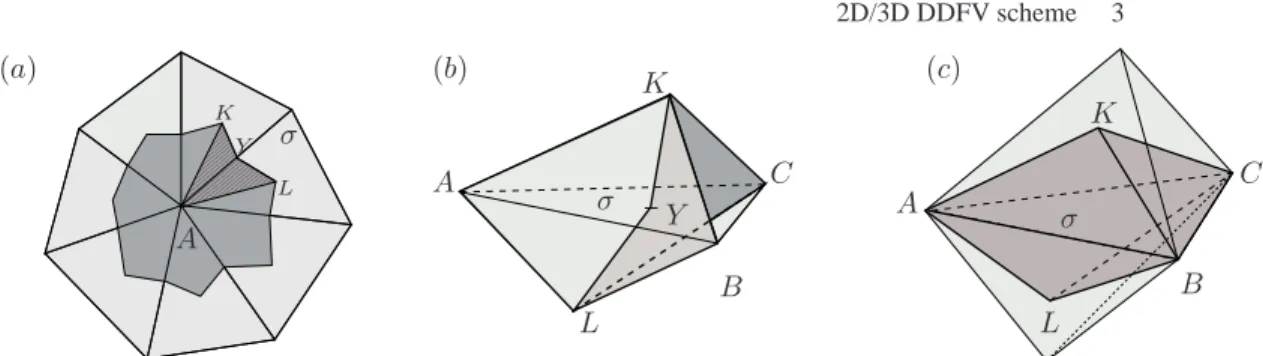
(a) (b) (c) A σ K L Y A C B L K Y σ A C B L K σ

Figure 1.(a) Two dimensional case, definition of PA,σ (hatched dark grey) andPA

(dark grey).(b) Three dimensional case, definition of PA,σ for an internal interface

σ = CK|CL = ABC. (c) Three dimensional diamond cell Dσ (dark grey).Dσ =

Dσ,K∪ Dσ,L,Dσ,K is the part aboveσ whereas Dσ,Lis the part underneathσ.

internal interface and let Y be σ’s centre. In dimension 2, PA,σ is the quadrilateral

AK1Y K2. In dimension 3, letB and C be the two other vertices of σ (σ = ABC).

Then PA,σ is the reunion of the two pyramids having the same quadrilateral base

ABY C and K1,K2for apex :PA,σ= ABY CK1 ∪ ABY CK2. That definition has

obvious extension to the caseσ⊂ ∂Ω.

Remark that in dimension 2 the (interiors of the) dual cells are disjoints and reco-ver the whole domain, thereforeP

A∈VPA = Ω. Whereas in dimension 3 the dual

cells are no more disjoints, if A and B are two vertices of the same interface σ, PA,σ∩PB,σ 6= ∅. Actually the dual cells now recover exactly twice the whole domain,

so thatP

A∈VPA= 2Ω.

To every interfaceσ∈ I is associated one diamond cell Dσ. For an internal

inter-faceσ= CK|CL, it is defined asDσ = Dσ,K∪ Dσ,LwhereDσ,K,Dσ,Lare the two

triangles/pyramids with baseσ and apex K and L respectively, as depicted on figure 2.1. In the case of a boundary interface σ ⊂ ∂Ω, Dσ is a simple triangle/pyramid,

Dσ= Dσ,K. TheDσ,Kwill be called sub-diamond cells.

To this different types of cells are associated the following types of data :

A discrete vector field Xh(resp. discrete tensorGh) is a vector (resp. matrix)

function, piecewise constant on each sub-diamond cellDσ,K. To each internal

inter-faceσ = CK|CLare associated two vectors Xσ,K and Xσ,L (resp. matricesGσ,K

andGσ,L) on each side ofσ. Gσ,Kis always assumed symmetric positive definite. We

shall say that Xhis conservative relatively toGhif (nσbeing a normal toσ) :

∀σ ∈ I such that σ = CK|CL : Gσ,KXσ,K· nσ= Gσ,LXσ,L· nσ, (3)

A discrete scalarϕhis the data of two sets of scalars(ϕA)A∈V,(ϕK)_CK∈C

asso-ciated to the vertices and primal cells centres respectively.

A DDFV function is a scalar function ϕ˜h, piecewise affine on AYσK (resp.

ABYσK) whenever σ ∈ I, A ∈ V (resp. A, B ∈ V ) is (are) vertex(es) of σ in

4 1re _{soumission à fvca5.}

2.2. The discrete operators and the problem discretisation

The discrete divergence divhof a discrete vector field Xhis the discrete scalar :

(divhXh)A= 1 PA Z ∂PA X_{h· n∂P} Ads , (divhXh)K = 1 CK Z ∂CK X_{h· n∂C} K ds, (4)

where n∂E is the outward unit normal on the boundary of the polygonal/polyhedral

element E. That definition makes sense because there are no discontinuities of Xhon

the edges/faces of primal and dual cells.

The discrete gradient of a DDFV functionϕ˜his the discrete vector field :

(∇hϕ˜h)σ,K = 1 Dσ,K Z Dσ,K ∇ϕhdx . (5)

The discrete gradient for a discrete scalar is defined below, for implementation, a practical formulation is given in appendix A.

Definition 2.1. Let us consider a discrete scalarϕhsuch thatϕA= 0 for all A ∈ VD

and a discrete tensorGh. Then there exists a unique DDFV functionϕ˜hsuch that :

∀ A ∈ V : ˜ϕh(A) = ϕA, ∀ CK∈ C : ˜ϕh(K) = ϕK,

∀ σ ∈ ID_{: ˜ϕ}

h(Yσ) = 0 , ∀ σ ∈ IN : Gσ(∇hϕ˜h)σ· nσ= 0 ,

and such that∇hϕ˜his conservative relatively toGh, as defined in (3).

Relatively toGh, the discrete gradient ofϕhis defined as∇hϕh= ∇hϕ˜h.

The previously defined discrete operators fulfil a duality property called discrete

Green formula by analogy with the continuous case :

Proposition 2.2. Let Gh a discrete tensor,ϕh a discrete scalar and consider the

DDFV functionϕ˜h associated toϕhrelatively toGh. If Xhis a discrete vector field

that satisfy Xσ,K· nσ = Xσ,L· nσon every internal interfaceσ= CK|CL, then :

Z Ω (∇hϕh) · Xhdx= − 1 d X CK∈C ϕK(divhXh)KCK− d− 1 d X A∈V ϕA(divhXh)APA + Z ∂Ω ˜ ϕh|∂ΩXh|∂Ω· n∂Ωds (6)

The consequence is the following :

Proposition 2.3. The right hand sidef in (1) being discretised in some discrete scalar fh, we look for a discrete scalarϕhsuch that :

∀A ∈ VD

: ϕA= 0 , ∀σ ∈ IN : Gσ(∇hϕh)σ· nσ= 0 , (7)

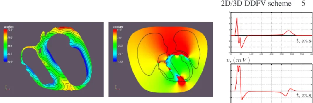
0 50 100 150 200 250 300 350 400 −4 −2 0 2 4 6 8 0 50 100 150 200 250 300 350 400 −6 −4 −2 0 2 4 v,(mV ) t, ms t, ms

Figure 2. (left) Simulation ofv : isochrons (ms )for the excitation wave on a 2D

ven-tricles slice mesh coming from MRI segmented images, 485000 degrees of freedom. (middle) Computation ofϕ at time t = 50ms. The four domain are separated with

black lines (ventricles, ventricles cavities, lungs and torso remaining). (right) Simula-ted ECG for two leads (V1 and V 2) located on the body surface.

Such aϕhsatisfies the transmission conditions (2) in a discrete sense by construction.

If ID _{6= ∅, (7) has a unique solution. The resulting numerical linear problem to}

invert is moreover symmetric positive definite. The Neumann problem (ID_{= ∅) has a}

solution iff1 d P CK∈CfKCK+ d− 1 d P

A∈VfAPA= 0. The linear problem to invert

is now symmetric positive, its kernel is composed of the discrete scalarψhsuch that

ψA= C1,ψK = C2.

3. Application

The bidomain model (see e.g. [KEE 98]) describes the electrical activity of the heart. It involves two compartments : the intra/extra cellular mediums, and models a trans-membrane potentialv = ϕi− ϕ, difference between the intra/extra cellular

potentials respectively. We use here the modified monodomain model (see [CLE 04]), v(x, t) is given through a reaction diffusion system involving a second variable w(x, t) ∈ RN _{that describes the cells membrane activity (N is up to 20). It is used to simulate}

the normal propagation of excitation potential wave fronts (v passing from a rest value to a plateau value) and de-excitation, see figure 3. It reads :

AmCm

∂v

∂t + AmIiOn(v, w) = div(G1∇v) + Iapp(x, t) , ∂m

∂t = g(v, w). (8) Am,Cmare constants,G1is a non constant anisotropy tensor described below,Iion,

g are reaction terms and Iappa source term (applied current) that activates the

sys-tem. The electrocardiograms (ECG) is the body surface potential resulting from that cardiac electrical activity. It is the trace on the torsoT boundary ∂T of the extracel-lular potentialϕ. In the extra cardiac T − H, ϕ(x, t) is given by a Poisson equation div(GT∇ϕ) = 0, where GT is isotropic heterogeneous between the different tissue

layers conductivities (lungs, blood...). In the heartH, current balance between the in-tra and exin-tra cellular compartments gives div(G2∇ϕ) = −div(G3∇v). The tensors

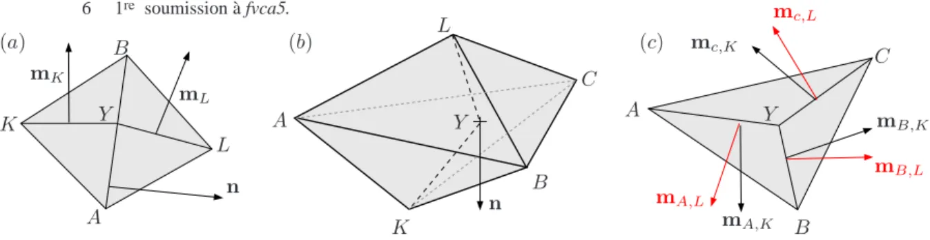
6 1re _{soumission à fvca5.} (a) n L K Y A B m_K m_L (b) n L K Y A B C (c) Y A B C m_c,K m_c,L m_B,K m_B,L m_A,K m_A,L

Figure 3. Notations for the gradient definition.(a) Two dimensional case : interface σ = AB = CK|CL of centre Y , the three vectors n, mK, mL have unit length

and are respectively orthogonal toσ, Y K, Y L. Three dimensional case.(b) Interface σ= ABC = CK|CL of centreY , n its unit normal from CK towardsCL.(c) Same

interfaceσ view from above, all vectors have unit length, mA,K, mB,K and mC,K

are orthogonal toAY K, BY K and CY K respectively ; same thing for mA,L, mB,L

and mC,Lby turningK into L.

Gitake into account the fibrous organisation of the heart. They read the same

aniso-tropic/non constant form :Gi(x) = P−1(x) ˜GiP(x), where ˜Gi = Diag(gli, gti) is a

reference matrix :gl

i,gitbeing the longitudinal/transverse conductivities along/across

the cardiac fibres.P(x) then is a change of basis matrix from the Frenet basis atta-ched to the fibre direction at pointx. On the whole domain T , this results in one global elliptic equation per time instantt :

div(G∇ϕ(t)) = f (v(t)) , f(v(t)) = (

0 inH

−div(G3∇v(t)) in T − H

, (9)

completed with the transmission conditions (2) on the heart/torso boundary and also on the interface between different tissue layers, and also with a Neumann boundary condition on∂T (no current flow out of the body). In that problem, v(x, t) is an entry coming from a first computation on the heart previously described.

We then discretised (9) using the DDFV scheme. Our domainT is a torso slice mesh coming from MRI segmented data and counting 600 000 degrees of freedom. The do-main is divided in four parts : the heart, the ventricles cavities (filled in with blood), the lungs and the remaining torso. each part having the different previously described conductivity properties.ϕ is computed on T at each ms, the ECG body surface po-tential is recorded at 6 leads located on the torso boundary, see figure 3. On a whole cardiac cycle (≃ 600 ms), 600 computation are thus performed. That computation ne-cessitates the inversion of an ill-conditioned symmetric positive linear system at each ms. For this a Gm-Res solver combined with a basic SSOR preconditioning has been used.

A. Discrete gradient implementation

With the notations of def. 2.1 and of figure A, the expression of∇hϕhis :

d= 2 : 2Dσ,K(∇hϕh)σ,K = ( ˜ϕ(Y ) − ϕK) σn + (ϕB− ϕA) KY mK

d= 3 : 3Dσ,K(∇hϕh)σ,K = ( ˜ϕ(Y ) − ϕK) σn + (ϕB− ϕC) AY KmA,K

+ (ϕC− ϕA) BY KmB,K+ (ϕA− ϕB) CY KmC,K

It involves the DDFV functionϕ˜hin def. 2.1, whose definition is completed by :

d= 2 : ˜ϕh(Y ) = αϕK+ (1 − α)ϕL+ k(ϕB− ϕA) d= 3 : ˜ϕh(Y ) = αϕK+ (1 − α)ϕL+ kA(ϕB− ϕC) + kB(ϕC− ϕA) + kC(ϕA− ϕB) . with : α−1= 1 +Dσ,K Dσ,L n_Gσ,Ln n_Gσ,Kn k= LY σ m_LGσ,Ln Dσ,L Dσ,K n_Gσ,Kn_{+ nGσ,L}n −KY σ m_KGσ,Kn Dσ,K Dσ,L n_Gσ,Ln_{+ nGσ,K}n kZ = ZY L σ m_Z,LGσ,Ln Dσ,L Dσ,K n_Gσ,Kn_{+ nGσ,L}n −ZY K σ m_Z,KGσ,Kn Dσ,K Dσ,L n_Gσ,Ln_{+ nGσ,K}n , Z= A, B, C.

For boundary interfaces this expression is adapted as follows. Forσ∈ ID_{, ˜}

ϕh(Y ) =

0. For σ ∈ IN_{, one suppresses}

Dσ,Lby statingL= Y and Gσ,L = 0.

B. Bibliographie

[AND 06] ANDREIANOV B., BOYER F., HUBERT F., « Discrete-duality finite volume schemes for Leray-Lions type elliptic problems on general 2D meshes », Num. Methods for PDE, vol. 23, no

1, 2006, p. 145 - 195.

[CLE 04] CLEMENTSJ., NENONENJ., HORACEKM., « Activation Dynamics in Anisotropic Cardiac Tissue via Decoupling », Annals of Biomed. Eng., vol. 32, no

7, 2004, p. 984-990. [DEL 07] DELCOURTE S., DOMELEVO K., OMNÈS P., « A Discrete Duality Finite Vo-lume Approach to Hodge Decomposition and div-curl Problems on Almost Arbitrary Two-Dimensional Meshes », SIAM Num. Anal., vol. 45, no

3, 2007, p. 1142-1174.

[DOM 05] DOMELEVOK., OMNÈSP., « A finite volume method for the Laplace operator on almost arbitrary two-dimensional grids », M2AN, vol. 39, no

6, 2005, p. 1203-1249. [HER 00] HERMELINEF., « A finite volume method for the approximation of diffusion

ope-rators on distorted meshes. », J. Comput. Phys., vol. 160, no

2, 2000, p. 481-499. [HER 03] HERMELINEF., « Approximation of diffusion operators with discontinuous tensor

coefficients on distorted meshes. », Comput. Methods Appl. Mech. Eng., vol. 192, no

16-18, 2003, p. 1939-1959.

8 1re _{soumission à fvca5.}

[HER 07] HERMELINEF., « Approximation of 2-D and 3-D diffusion operators with variable full tensor coefficients on arbitrary meshes », Comput. Methods Appl. Mech. Eng., vol. 196, no

1, 2007, p. 2497-2526.

[KEE 98] KEENERJ., SNEYDJ., Mathematical Physiology, Springer-Verlag, 1998.

[LAD 68] LADYZENSKAJAO. A., URAL’CEVAN. N., Equations aux dérivées partielles de type elliptique, Monographies Universitaires de Mathématiques, No. 31, Dunod, Paris, 1968.