En vue de l'obtention du
DOCTORAT DE L'UNIVERSITÉ DE TOULOUSE
Délivré par :
Institut National Polytechnique de Toulouse (INP Toulouse) Discipline ou spécialité :
Micro-ondes, Électromagnétisme et Optoélectronique
Présentée et soutenue par :
M. JALAL AL ROUMY
le mardi 20 septembre 2016
Titre :
Unité de recherche : Ecole doctorale :
ANALYSIS OF THE DIFFERENT SIGNAL ACQUISITION SCHEMES OF
AN OPTICAL FEEDBACK BASED LASER DIODE INTERFEROMETER
Génie Electrique, Electronique, Télécommunications (GEET)
Laboratoire d'Analyse et d'Architecture des Systèmes (L.A.A.S.) Directeur(s) de Thèse :
M. THIERRY BOSCH M. JULIEN PERCHOUX
Rapporteurs :
M. MAURIZIO DABBICCO, UNIVERSITA DEGLI STUDI DI BARI M. SANTIAGO ROYO, CD6 Universitat Politecnica Catalunya
Membre(s) du jury :
1 M. MICHEL LEQUIME, ECOLE CENTRALE DE MARSEILLE, Président
2 M. JULIEN PERCHOUX, INP TOULOUSE, Membre
2 M. PHILIPPE ARGUEL, UNIVERSITE PAUL SABATIER, Membre
iii
Acknowledgments
I would like to express my admiration and gratitude to my Prof. Thierry Bosch, thesis advisor, for granting me the opportunity of being part of the OSE research group. His scientific skills and perpetual willingness to listen have made an enormous contribution to this work, while his humanity and advices allowed me to overcome the hard times along this journey.
All my respect and compliments go to Dr. Julien Perchoux for co-advising my work. Always full of sureness, his insights and friendship increased the confidence on my background knowledge and empowered the joy of becoming proficient in the domain of optical sensing. He was so patient with me and provided me with so many helpful advices whenever I struggled due to home sickness or worrisome about the situation of my family.
I would also like to thank Mr. Maurizio Dabbicco and Mr. Santiago Royo for accepting to be the reviewers of my thesis. I am thankful for any advice and suggestions from all the jury members.
The financial support provided by the French Government which was directed during the three years by the Campus France, is gratefully acknowledged. My special thanks go to the Academic Cooperation Division in the French Consulate in Jerusalem for selecting me to this program.
I’m grateful to all the researchers and staff of this group for their kindness and the positive work ambiance all these years, Marc Lescure, Michel Cattoen, Francoise Lizion, Olivier Bernal, Francis Bony, Hélène Tap, Han-Cheng Seat and Adam Quotb. I'm also grateful to Clement Tronche and Francis Jayat for their great help in conducting the experiments, and Emmanuelle Tronche for her help in the management stuff.
I treasure the time spent with all my fellow PhD students, Antonio Luna Arriaga, Bendy Tanios, Lucas Perbet, Blaise Mulliez, Mohanad Albughdadi, Haris Apriyanto, Laura Le Barbier, Lavinia Ciotirca, Evelio R. Miquet, Yu Zhao, Raul Da Costa Morerira and Patricio Fernando Urgiles Ortiz. My thoughts and
iv
appreciation for the many other great people who I had the pleasure to know and exchange opinions in this research centre, Gautier, Usman, Laurent, Luc Eric, Sabine, Florentin and Jose Luis.
The work on this manuscript has been accomplished with the support and encouragement from the people who has been with me since the beginning, my parents who have devoted their life to make me grow integrally as well as my brother and sisters. There are no words to thank the precious time that you gave me, I dedicate this work to you.
v
Table of Contents
Acknoledgment ... iii
Table of Contents ... v
List of Figures ... vii
List of Tables ... xiii
General Introduction ... 1
1 Principle and Applications of Optical Feedback Interferometry ... 5
1.1 Introduction to the History of Optical Feedback Interferometry ... 6
1.2 Principle of the Optical Feedback Interferometry ... 10
1.2.1 Model of coupled cavities ... 12
1.3 Applications of Optical Feedback Interferometry... 22
1.3.1 Typical sensing applications ... 23
1.3.2 High sensitive sensing applications ... 30
1.4 Conclusion ... 34
2 Modelling of Optical Feedback Interferometric Signals ... 35
2.1 Re-demonstration of OFI Rate Equations Model ... 38
2.1.1 Standalone laser diode... 39
2.1.2 Laser diode subject to optical feedback ... 49
2.2 Amplitudes of LV and PD OFI signals ... 53
2.2.1 Photodetected signal ... 54
2.2.2 Voltage signal ... 60
2.3 Analysis of the Front PD Signal ... 64
2.4 Conclusion ... 70
3 Experimental Validation of the OFI Signal Modelling ... 71
3.1 Validation of the Model for Single-mode Laser Diodes ... 72
3.1.1 Description of the Experimental Setup ... 72
3.1.2 Detailed description and characterization of both laser diodes ... 75
3.2 Experimental Validation ... 81
3.2.1 A DFB laser diode subject to optical feedback ... 81
vi
3.3 OFI Signals Strength Evolution for Multimode Lasers ... 95
3.4 The Case of the Front PD Signal ... 100
3.4.1 Comparison of the amplitudes of the front and the back PD signals .. ... 100
3.4.2 Phases of front and back PD signals ... 104
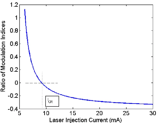
3.4.3 Ratio of modulation indices ... 109
4 Improvement of the OFI sensor sensitivity using multiple acquisition schemes ... 111
4.1 Description of the Experimental Setup ... 113
4.2 Theoretical Background ... 114
4.2.1 Noise sources in different acquisition schemes ... 114
4.2.2 The applied signal processing techniques ... 115
4.2.2 Validation on ideal signals ... 119
4.3 Experimental Results ... 122
4.3.1 Different feedback levels ... 123
4.3.2 Different injection currents ... 135
4.4 Conclusion ... 139
General Conclusion ... 134
Bibliography ... 147
List of Publications ... 165
vii
List of Figures
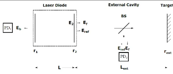
Fig. 1.1: A comparison between a conventional interferometer (left) and the OFI interferometer (right) ... 10 Fig. 1.2: A schematic diagram of a laser commercial package with a built-in monitoring photodiode ... 11 Fig. 1.3: A simple Fabry-Pérot model of the solitary laser diode. ... 12 Fig. 1.4: The three-mirror model of a laser diode subject to optical feedback .... 14 Fig. 1.5: The reduced model of laser diode subject to optical feedback . ... 15 Fig. 1.6: The round-trip phase change against the lasing frequency change simulated for different values of the feedback parameter C ... 20 Fig. 1.7: The regimes of feedback levels at different power ratios ... 22 Fig. 1.8: The displacement of a target can be retrieved from processing the OFI signal acquired for a target moving along the optical path of a laser diode: (a) basic representation of the displacement measurement setup, and (b) a sinusoidal displacement with sawtooth-like fluctuations ... 24 Fig. 1.9: a) Laser Doppler velocimetry demonstration with a VCSEL sensor: a) basic representation of the velocity measurement setup and b) an OFI signal spectrum ... 27 Fig. 1.10: Optical power variations and their corresponding beat frequencies for a triangular injection current ... 29 Fig. 1.11: Schematic diagram of the of the acoustic filed measurement setup ... 31 Fig. 1.12: Ppropagation of the acoustic field with the ultrasonic transmitter propagating the field into free space; Left: Measured, Right: Simulation ... 32 Fig. 1.13: Experimental setup for edge filter enhanced self-mixing interferometry (ESMI) experiments ... 33 Fig 2.1: A block diagram of the laser diode and the photodiodes ... 36 Fig 2.2: Flowchart that illustrates the main stages undergone to derive the OFI model equations ... 37
Fig. 2.3: Evolution of the PD and LV OFI Signals strengths with laser injection current ... 63 Fig. 2.4: Evolution of the PD and LV OFI Signals strengths with the operating temperature ... ... 64
viii
Fig 2.5: A schematic representation of the phase relationship model ... 65 Fig 2.6: The ratio of modulation indices as a function of injection current ... 69 Fig 2.7: Evolution of the front and the back PD signals normalised strengths with laser injection current ... 69 Fig. 3.1: Photography of the experimental setup for measuring velocity of a rotating disk: 1) a micrometric 3-axis mechanical stage, 2) lens, 3) neutral density, 4) rotating disk (target), 5) needle, 6) laser driver, and 7) amplifier ... ... 73 Fig. 3.2: Block diagram of the experimental setup inside the climatic chamber . 73 Fig. 3.3: Output optical power of the DFB laser as a function of laser injection current measured at different operating temperatures (ranging from -40 ̊ C to 80 ̊ C in steps of 5 ̊ C) ... 77 Fig. 3.4: Measured (solid lines) and fitted (dashed and dotted lines) slope efficiency and threshold current of the DFB laser diode as a function of the operating temperature. The upper slope efficiency curve is the maximum while the lower one is the average ... 78 Fig. 3.5: Output optical power of the VCSEL as a function of laser injection current measured at different operating temperatures (ranging from 0 ̊ C to 80 ̊ C in steps of 5 ̊ C). ... 79 Fig. 3.6: Slope efficiency and threshold current of the VCSEL as a function of the operating temperature ... 80
Fig. 3.7: The Doppler signal spectrum. The inset shows the fitting of the measured spectrum (black) to a combination of a Gaussian function and a linear function fitting the noise floor (green) ... 82 Fig. 3.8: Evolution of the PD signal amplitude of the DFB with laser injection current: measured (red solid); modelled (constant slope efficiency of an ideal laser diode, green dashed); modelled (actual slope efficiency, blue solid). ... 83 Fig. 3.9: Evolution of the LV signal amplitude of the DFB with laser injection current: measured (red solid); modelled (constant slope efficiency of an ideal laser diode, green dashed); modelled (actual slope efficiency, blue solid). ... 83 Fig. 3.10: Evolution of the PD signal amplitude of the DFB with the operating temperature: measured (red solid); modelled (actual slope efficiency, blue solid). ... 85
ix Fig. 3.11: Evolution of the LV signal amplitude of the DFB with the operating temperature: measured (red solid); modelled (actual slope efficiency, blue solid). ... 85 Fig. 3.12: PD signal strength of the DFB laser diode as a function of the injection current and the operating temperature: (a) measured and (b) modelled ... 87 Fig. 3.13: LV signal strength of the DFB laser diode as a function of the injection current and the operating temperature: (a) measured and (b) modelled ... 88
Fig. 3.14: Evolution of the PD signal amplitude of the VCSEL with laser injection current at 20 ̊C: measured (red solid); modelled (constant slope efficiency of an ideal laser diode, green dashed); modelled (actual slope efficiency, blue solid). .. ... 89 Fig. 3.15: Evolution of the LV signal amplitude of the VCSEL with laser injection current: measured (red solid); modelled (constant slope efficiency of an ideal laser diode, green dashed); modelled (actual slope efficiency, blue solid). ... 90 Fig. 3.16: Evolution of the PD signal amplitude of the VCSEL with the operating temperature: measured (red solid); modelled (actual slope efficiency, blue solid). ... 91 Fig. 3.17: Evolution of the LV signal amplitude with the operating temperature of the VCSEL: measured (red solid); modelled (actual slope efficiency, blue solid) ... 91 Fig. 3.18: PD signal strength of the VCSEL as a function of the injection current and the operating temperature: (a) measured and (b) modelled ... 93 Fig. 3.19: LV signal strength of the VCSEL as a function of the injection current and the operating temperature: (a) measured and (b) modelled ... 94 Fig. 3.20 The two-mode operation of the VCSEL a) the operating wavelength and b) the total output power and detected power of each mode. ... 96 Fig. 3.21: Evolution of the PD OFI signal amplitude with the laser injection current in the two-mode VCSEL. Solid blue line: simulated taking into account the actual slope efficiency; dashed line: simulated with constant slope efficiency; red solid line: measured. ... 97 Fig. 3.22: Evolution of the amplitude of the voltage OFI signal with laser injection current in the two-mode VCSEL. Solid blue line: simulated taking into account the actual slope efficiency; dashed line: simulated with constant slope efficiency; red solid line: measured. ... 98
x
Fig. 3.23: Evolution of the PD OFI signal amplitude with laser injection current in the two-mode VCSEL ... 99 Fig. 3.24: Evolution of the voltage OFI signals amplitudes with injection current for multimode laser diodes ... 99 Fig. 3.25: Experimental setup used for the simultaneous measurement of the front and back PD signals ... 101 Fig. 3.26 Back (upper plots) and front (lower plots) PD signals at different bias currents: a) I = 6 mA, PD signals are in-phase, b) I = 9 mA, front PD signal vanishes, c) I = 16 mA, signals are out-of-phase ... 102 Fig. 3.27 Evolution of the amplitudes of the back (blue trace) and front (green trace) PD signals with laser injection current at different attenuation levels: top) No neutral density is introduced to the optical path; middle) Attenuation level is 16 dB; bottom) Attenuation level is 20 dB. ... 103 Fig. 3.28 Photocurrents as a function of the injection current measured at different attenuation levels (purple solid line for external photodiode, and golden solid line for the internal photodiode) ... 104 Fig. 3.29 The phase difference as a function of frequency at: a) 7 mA, and b) 27 mA. ... 105 Fig. 3.30 Histogram of the phase difference at: a) 7 mA, and b) 27 mA. ... 106 Fig. 3.31 Histogram of the corrected phase difference at: a) 7 mA, and b) 27 mA. ... 107 Fig. 3.32 Phase differences as a function of the laser injection current measured at different attenuation levels (blue solid line for the case of no attenuation; green solid line for the case of 16 dB attenuation; and red solid line for the case of 20 dB attenuation). ... 108 Fig. 3.33 Ratio of modulation indices as a function of the injection current both modelled (black solid line) and measured at different attenuation levels (blue solid line for the case of 0 dB attenuation; green solid line for the case of 16 dB attenuation; and red solid line for the case of 20 dB attenuation). ... 110 Fig. 4.1: Spectrum of a noisy sinusoidal signal with a frequency of 1 kHz and an amplitude of 1, accompanied by a white Gaussian noise with a standard deviation of 0.2. The SNR in decibel is measured as the difference between the signal amplitude at 1 kHz and the average noise level elsewhere ... 112
xi Fig. 4.2: The sum and the difference SNRs of the input signals as a function of the phase shift (solid blue is the sum, and solid green is the difference). The SNRs of the input signals are equal and are normalised at 0̊ ... 121 Fig. 4.3: SNRs of OFI signals obtained at 6.5 mA for different feedback levels (solid red: LV signal, solid black: back PD signal, and solid blue: front PD signal). ... 124 Fig. 4.4: SNRs of the output signals obtained from the autocorrelation of the OFI signals at 6.5 mA for different optical feedback levels (solid blue: obtained values, and dashed red: expected values) ... 125 Fig. 4.5: SNRs of the cross-correlation of the OFI signal pairs obtained at 6.5 mA for different feedback levels (solid blue: obtained values, and dashed red: expected values) ... 126 Fig. 4.6: SNRs of either the addition or the subtraction of the OFI signal pairs obtained at 6.5 mA for different attenuation levels (solid blue: obtained values, and dashed red: SNRs of the OFI signals) ... 128 Fig. 4.7: SNRs of OFI signals obtained at 20 mA for different feedback levels (solid red: LV signal, solid black: back PD signal, and solid blue: front PD signal) ... 130
Fig. 4.8: SNRs of the output signals obtained from the autocorrelation of the OFI signals at 20 mA for different optical feedback levels (solid blue: obtained values, and dashed red: expected values) . ... 131 Fig. 4.9: SNRs of the cross-correlation of the OFI signal pairs obtained at 20 mA for different feedback levels (solid blue: obtained values, and dashed red: expected values) ... 132
Fig. 4.10: SNRs of either the addition or the subtraction of the OFI signal pairs obtained at 20 mA for different attenuation levels (solid blue: obtained values, and dashed red: SNRs of the OFI signals). . ... 134
Fig. 4.11: SNRs of OFI signals as a function of laser injection current (solid red: LV signal, solid black: back PD signal, and solid blue: front PD signal). ... 135
Fig. 4.12: SNRs of the output signals obtained from the autocorrelation of the OFI signals measured at different laser injection currents (solid blue: obtained values, and dashed red: expected values).. ... 136
xii
Fig. 4.13: SNRs of the cross-correlation of the OFI signal pairs as a function of laser injection current (solid blue: obtained values, and dashed red: expected values). ... 137
Fig. 4.14: SNRs of either the addition or the subtraction of the OFI signal pairs obtained at different laser injection currents (solid blue: obtained values, and dashed red: SNRs of the measured OFI signals). ... 138 Fig. 4.15: SNRs of the outputs of the different signal processing techniques (AC: autocorrelation, XC: cross-correlation, sum and difference) of the different OFI input signals (L: LV signal, B: back PD signal, and F: front PD signal) acquired at 6.5 mA for different attenuation levels (red solid: 0 dB, black solid: 12 dB, and blue solid: 20 dB) ... 139 Fig. 4.16: SNRs of the outputs of the different signal processing techniques (AC: autocorrelation, XC: cross-correlation, sum and difference) of the different OFI input signals (L: LV signal, B: back PD signal, and F: front PD signal) acquired at 20 mA for different attenuation levels (red solid: 0 dB, black solid: 12 dB, and blue solid: 20 dB). ... 140 Fig. 4.17: Comparison of the SNRs of both the cross-correlation and the difference of the LV and back PD signals as a function of the laser injection current (solid red: cross-correlation and solid blue: difference). ... 141 Fig. 4.18: Comparison of the SNRs of both the cross-correlation and the difference of the front and back PD signals as a function of the laser injection current (solid red: cross-correlation and solid blue: difference). ... 141
xiii
List of Tables
Table 1.1: The characteristics of the regimes of optical feedback levels. ... 21
Table 3.1: A comparison of the lasers’ absolute maximum ratings ... 76
Table 3.2: A comparison of the lasers’ important parameters ... 76
Table 3.3: Laser parameters used for the calculation of the model curves ... 109
Table 3.4: Comparisons of the fitted and the standard values of the ratio of the carrier densities at transparency ... 109
Table 4.1: Calculated and evaluated SNRs of the output signals ... 121
Table 4.2: Calculated and evaluated SNRs of the sum of the in-phase input signals ... 122
1
General Introduction
2
Optical feedback interferometry (OFI) is a promising sensing technique for both industrial and laboratory environments due to its simple optical setup when compared to other interferometric techniques. Typical sensing applications of OFI are the measurement of displacement, absolute distance, vibration and velocity of solid targets.
The OFI sensing technique allows to design compact, self-aligned and cost-effective sensors with a very good precision comparable with the one offered by the more accurate, yet more complicated and more expensive, conventional interferometric sensors. This comes from the fact that, in OFI sensors, there is no need for a separate receiving channel to first gather and then mix the back-reflected optical power from the remote target, which is the case in conventional interferometry. In the OFI sensing scheme, the back-reflected laser beam is coupled into the active laser cavity where it induces changes of the lasing frequency and the optical power of the laser diode. These perturbations, and in particular the power perturbation, are carrying information on the remote target and the external cavity.
The most recent and exciting applications proposed for OFI sensors concern the monitoring of fluid flows and the imaging of acoustic wave. In the case of fluid flows at the micro-scale, small particles such as red blood cells are flowing in semi-transparent ducts and are the remote targets that induce the Doppler shifted back-scattering inside the laser cavity. For the imaging of acoustic wave, the sensors measures the pressure induced change of the refractive index in the external cavity formed by the laser and a fixed diffusing target. Despite their complete different nature, these two applications encounter the same challenge: the changes in the measurable quantity (laser power or laser frequency) are extremely small and can easily be drowned into the noise thus constraining the sensor’s range of operation. In all applications requiring the detection of very small changes, OFI sensor signal strength is a key parameter which requires the full attention when designing the sensor. The objective of the present thesis is to describe both theoretically and experimentally the sensor parameters that impact directly the OFI signal amplitude.
3 OFI signals can be acquired by two different means: the first method is by observing the power fluctuations in the output optical power emitted from either the rear facet of the laser diode using the commonly built-in monitoring photodiode (denoted here as the rear PD signal) or the front facet using an external photodiode (denoted here as the front PD signal). The second method is by amplifying the variations in the laser junction voltage (denoted here as the LV signal). In this acquisition scheme, the laser diode acts simultaneously as: a light source, a micro-interferometer and a light detector. Actually, the latter method is the only measurement approach when a monitoring photodiode is not included in the laser diode package, as for example, when an array of laser diodes is used. Moreover, in the second configuration, the OFI sensor is reduced to the laser diode itself associated with a focusing lens, which is quite interesting for industrial applications as it opens up new possibilities for increased miniaturization of the sensor.
For both methods of signal acquisition in OFI sensors, in order to achieve the best performance, it is essential to maintain the maximum signal-to-noise ratio. Thus, this thesis proposes a simple mathematical model, applicable to single-mode laser diodes, which provides compact analytical expressions to quantitatively describe the dependence of OFI signal strength on the laser injection current. Due to the device-dependent nature of the optical feedback sensing scheme, we have limited our study to single-mode (transverse and longitudinal) laser diodes and only experimental results have been performed on multimode devices. The thesis manuscript has been written with the following order:
In the first chapter, an introduction to the OFI phenomenon is presented. The chapter consists of three major sections: a historical overview of the OFI phenomenon and the state-of-the art in this field is described in the first section. In the second section, the theoretical background required for a proper understanding of the phenomenon is presented. The expressions of the threshold gain, the emission frequencies and the phase condition are derived based on the equivalent cavity model. In the third section, various applications of the phenomenon are presented with a particular focus on the most demanding ones in term of signal strength.
4
The second chapter is dedicated to the demonstration of the analytical model that describes the evolution of the OFI signals strengths with the system parameters, and particularly the laser injection current. The derived model proposes an explanation to the experimentally observed divergent evolution of the PD and the LV signals with laser injection current. The chapter can be divided into three major sections: in the first section, a demonstration of the OFI rate equations for both the laser diode subject to optical feedback is presented. Those rate equations, and in particular the photon and the carrier densities, are then used as the basis for the derivation of the analytical model of OFI signals in the second section. The third section of this chapter investigates the phase relationship between the front and the rear PD signals as well as the ratio of their modulation indices expressed as a function of the laser injection current.
The third chapter consists of the experimental validation of the behaviour predicted by the analytical model that describes all three OFI signals. In the first section of the chapter, the model is experimentally validated for two different types of pure single-mode laser diodes: a distributed feedback (DFB) laser and a vertical-cavity surface-emitting laser (VCSEL), while in the second section, the model pertinence in the case of multimode laser diodes is evaluated: a transverse multimode VCSEL and a longitudinal multimode Fabry-Pérot (FP) type laser diode are thoroughly investigated.
In the fourth chapter, different signal processing techniques are applied to either two of the different OFI signals (the front PD signal, the rear PD signal and the LV signal) in search for any noticeable improvements in the characteristics of the signals, and in particular the SNR. The method is based on the hypothesis that acquisition of the same informative signal through two different sources should be emphasizing the signal while suppressing the noise. Autocorrelation, cross-correlation, and the simple arithmetic addition/subtraction operations were applied to a noisy sinusoidal reference signal, then to the experimentally obtained OFI signals.
Finally, a general conclusion is proposed and further evolution of the modelling effort and sensor improvement are discussed.
5
Chapter 1
Principle and Applications of Optical
Feedback Interferometry
Chapter 1: Principles and Applications of Optical Feedback Interferometry
6
1.1 Introduction to the history of optical feedback interferometry
The Optical Feedback Interferometry (OFI) phenomenon occurs when a back-scattered light from an external object mixes optically with the electric filed within the active cavity of the laser diode thus inducing variations in its emitted power as well as its spectral properties. One of the problems with the first lasers constructed in 1960 [1, 2] was the presence of multiple longitudinal modes of emission. To counter this problem, Kleinman and Kisliuk first proposed in 1962 that the mode structure of the laser could be modified through the addition of an external mirror [3]. Such arrangement was first demonstrated for a Helium-Neon (He-Ne) laser in the same year by Kogelnik and Patel [4]. Many subsequent works in the following years demonstrated that mode selectivity could be achieved with the addition of reflective elements inside or outside the laser cavity [5-11].
In 1963, King and Steward first demonstrated that optical feedback could also be used for metrology applications when they observed the variation of the output power of a He-Ne laser with the distance to the external mirror [12]. The output power changes were periodic functions of the distance to the external mirror with a period of half the laser’s wavelength, a behaviour that was used later in many other He-Ne laser interferometers to measure velocity [13] or the refractive index [14-21] and density of plasma [22-29]. In 1972, Wheeler and Fielding first observed that the optical feedback interference fringes could also be monitored as a change in the voltage across the discharge tube [29], interestingly highlighting the ability to perform interferometry using only the laser itself without any extra photodetector.
Meanwhile, in 1964 Yeh and Cummins first performed a series of experiments where a reference beam from the laser and the light scattered from a fluidic chip were coherently mixed onto an external photodiode (PD) to determine the flow rate using the Doppler-Fizeau effect [30, 31]. In this technique, the optical components should be accurately aligned to ensure that the reference and scattered beams are nearly parallel when mixed onto the PD [32], which, in practice, is a difficult task. In 1968, Rudd reported the first auto-aligned configuration using a He-Ne laser when he experimentally proved that the mixing of the scattered and reference beams could take place inside the laser cavity and detected with a PD at
1.1 Introduction to the History of Optical Feedback Interferometry
7 the rear facet of the laser, demonstrating the measurement of velocity by exploiting the Doppler frequency shift [32]. Since then, the interest to use OFI as a reliable technique for instrumentation was revealed.
Those early demonstrations of the OFI were performed with the large and bulky He-Ne lasers. In 1962, the more compact and lower cost semiconductor lasers were first constructed, and just like the first gas lasers they were also exhibiting multiple modes of emission [33-36]. In 1964, Crowe and Craig first showed that the linewidth of the lasing spectrum could be reduced or even further that the single-mode emission could be achieved using the optical feedback [37]. In 1968, the change of the threshold carrier density of the semiconductor lasers due to the optical feedback was shown by Bachert and Raab [38] as well as Morosov et al. who also observed that this change was dependent on the distance to the external mirror [39]. Furthermore, Morosov reported that the influence of the optical feedback on the dynamical properties of the laser diode, and in particular the oscillating frequency.
In 1969, Broom discovered that a considerable enhancement in the intensity noise of the output power at the relaxation oscillation frequency as well as the noise of the voltage across the laser junction could be achieved when the spacing between the longitudinal modes in the external cavity was equal to the relaxation oscillation frequency of the laser diode [40]. This work as well as a subsequent theoretical analysis in 1970 [41] showed that the dynamic behaviour of the laser diode with optical feedback was also dependent on the strength of the light coupling from the external cavity.
Despite all these experimental observations, there was no theoretical model that could accurately describe the origins of the dynamical operation of semiconductor lasers with optical feedback until 1980, when Lang and Kobayashi showed that the changes in the carrier density of the laser diode due to optical feedback induce a modification of the refractive index, which in turn leads to a change in the lasing frequency [42].
The desire to use semiconductor laser diodes in optical communication systems greatly motivated the great interest in their spectral and dynamical properties. For proper and adequate long-distance light propagation, low loss optical fibres are
Chapter 1: Principles and Applications of Optical Feedback Interferometry
8
used which require the light from the semiconductor laser diode to be properly coupled in. In 1978, Ikushima and Maeda showed that the back-reflected light into the laser from the optical fibre can lead to periodic peaks in the noise floor of the output power spectrum, with a frequency spacing dependent on the length of the fibre [43]. Furthermore, in 1979, Hirota and Suematsu [44] first demonstrated that optical feedback from optical fibres can increase the intensity noise of the semiconductor laser, which has a major effect on the performance of fibre-optic communication systems as it can limit the transmission distance and maximum possible bit rate [45]. Thus, many researchers have often considered optical feedback in laser diodes as a nuisance and an undesirable phenomenon.
On the contrary, other researchers realised the possible use of optical feedback in semiconductor laser diodes for many applications, which was first demonstrated in 1975 by Seko et al. who proposed to use the change in the laser output power due to optical feedback for data storage applications [46]. In 1976, Mitsuashi et al. proposed that the same could be achieved by monitoring the voltage across the laser junction [47]. More in-depth experiments were performed and theoretical models were proposed to determine the amplitude of the voltage change due to optical feedback by Burke et al. in 1978 [48] and Mitsuashi et al. in 1981 [49]. The awareness of the ability to use that optical feedback in semiconductor lasers for metrology applications was rising by this time. In 1980, Dandridge et al. first presented an acoustic laser diode sensor capable of detecting sinusoidal displacements as small as 90 µm [50]. Meanwhile, more properties of OFI were discovered in other types of lasers: in 1984, Churnside used optical feedback in a CO2 laser to measure velocity where he demonstrated an enhancement in the modulation depth near the lasing threshold [51, 52].
This sparked a wide interest in the use of OFI for instrumentation and sensing applications. In 1986, a velocity measurement was demonstrated using a laser diode by Shinohara et al. [53] where he pointed out the capability to obtain the interferometric signal by monitoring the voltage variations across the laser junction. In 1987, Shimizu observed that the target’s direction of motion could be determined by examining the inclination of the power fringes [54]. A year later, Jentink et al. measured the velocity in a multi-mode laser diode, where they
1.1 Introduction to the History of Optical Feedback Interferometry
9 demonstrated the periodicity of the OFI signal with the distance to the target [55]. In 1991, Koelink et al. first measured the flow rate of blood using a fibre-coupled laser diode subject to optical feedback, which signified the potential use of OFI in many medical applications [56]. Recently, It is has been shown in 2005 by Zakian et al. that the OFI technique can also be used to determine the size of scattering particles [57].
Another application is the absolute distance measurement. In the displacement measurement, the target is moving and the displacement of the target is determined by counting the fringes for a constant injection current. However in the absolute distance measurement both the sensor and the target are fixed, so the lasing frequency is modulated through the modulation of the injection current so to observe signal fringes with a periodicity related to the target distance. This technique was first proposed by Beheim and Fritsch in 1986 [58].
Since these first demonstrations, the OFI technique has been widely used in the measurements of displacement [59-63], absolute distance [64-68], velocity of solid bulky targets [69-73] and flow rates [74-78] using different types of lasers. More applications include a rudimentary parallel self-mixing imaging system to measure the speed and distance to different points on a rotating disk [79-83] as well as scanning based imaging systems such as: near field scanning optical microscopes [84-89], surface profiling [90-94], modal analysis and defect detection of metallic plates [95-97], and three-dimensional range imaging [98-102].
Considering the exposed historical and the current state of research achievements, the OFI sensing scheme can be considered as an active research domain with high potential to incursion on both industrial and laboratorial applications. In the next section, the theoretical principle of OFI technique is introduced followed by a brief description of some major OFI sensing applications.
Chapter 1: Principles and Applications of Optical Feedback Interferometry
10
1.2 Principle of the Optical Feedback Interferometry
The OFI sensing scheme, which is also widely known as self-mixing or self-mixing interferometry, occurs when a small portion of the optical power of the lasing source is reflected and coupled into the laser cavity. This back-scattered and time-delayed electromagnetic field interacts (or mixes) with the one of the cavity resulting in changes in the laser properties such as: threshold gain, lasing frequency and output optical power. These changes carry information about the remote target which can be extracted through appropriate signal processing. A schematic illustration of the optical feedback interferometer is shown on the right side of Fig. 1.1, in comparison with a conventional Michelson interferometer. On one hand, all that is needed for an optical feedback interferometer is a laser diode as well as a collimating lens to focus the beam spot on the target surface. Some work has shown that the lens is not always necessary under certain conditions [103, 104]. Though not necessary, the monitoring photodiode that is already implemented inside the laser package is most common method used for the detection of the output power fluctuations due to OFI. On the other hand, additional optical components, such as: mirrors, splitters, isolators and etc., are necessary for the conventional interferometric system. Hence, the optical feedback interferometer is simpler, cheaper, self-aligned and more compact than the conventional interferometric techniques.
Fig. 1.1: A comparison between a conventional interferometer (left) and the OFI interferometer (right).
1.2 Principles of Optical Feedback Interferometry
11 In many commercial laser diodes, a monitoring photodiode is integrated inside the laser package to control the optical power emitted at the back facet, as shown in Fig. 1.2.
Fig. 1.2: A schematic diagram of a laser commercial package with a built-in monitoring photodiode.
However, optical feedback signals can still be obtained even without the monitoring photodiode by directly monitoring the voltage variations of the laser junction [60, 105]. This allows the deployment in OFI sensing of VCSEL based laser arrays where the integration of photodiodes is impractical [106], as well as the production of even smaller OFI sensors. Though, the signal-to-noise-ratio obtained from the voltage variations across the laser junction is usually lower than that obtained through the detection of the power variations [107].
A major difference between the optical feedback interferometers and the conventional interferometers is that the optical feedback interferences occur in an active medium with an imaginary refractive index whereas in conventional interferences are normally observed in free space, a passive medium. Therefore, the OFI sensor simultaneously acts as a power source, a micro-interferometer and as a light detector.
In order to further understand the subtleties of OFI, we consider the well documented model of coupled cavities, with the target as an external optical cavity. In this chapter we will present the rate equations of the laser diode subject to optical feedback based on those of the standalone laser diode that we will first present.
Chapter 1: Principles and Applications of Optical Feedback Interferometry
12
1.2.1 Model of Coupled Cavities
The standalone laser diode is simply modelled as a gain medium bounded by two mirrors. To account for the remote target and the subsequent optical feedback, a third mirror is added to the model resulting in what is called the three-mirror resonator.
1.2.1.1 Standalone laser diode
Due to its simple structure, the adopted model, shown in Fig. 1.3, is based on the Fabry-Pérot laser diode [108]. The laser diode is modelled as an active medium of effective refractive index of neff and length L, which is bounded by two
mirrors with field reflection coefficients of r1 and r2 respectively for the rear mirror and the front mirror.
Fig. 1.3: A simple Fabry-Pérot model of the solitary laser diode.
The time-varying electric field inside the laser cavity at any point along the z-axis is given by:
𝐸(𝑧, 𝑡) = 𝐸0. 𝑒𝑗𝜔𝑡. 𝑒−𝑗𝛽𝑧 (1.1)
Where E0 is the electric field amplitude, ω is the angular frequency, β = 2 𝜋 𝑛eff
𝜆 is
the phase constant, where λ = 𝑐𝜈 is the wavelength of the electric field, ν is the lasing frequency, and c is the speed of light in vacuum.
The electric field propagating inside the laser cavity will encounter a gain as the active medium has a power gain per unit length of g. A power loss per unit length of αs is assumed to account for the optical losses within the laser cavity.
1.2 Principles of Optical Feedback Interferometry
13 Taking into account for the power gain and losses, the time-independent term of electric field, E(z), from eq. (1.1) can be written as:
𝐸(𝑧) = 𝐸0. 𝑒0.5(𝑔−𝛼𝑠)𝑧. 𝑒−𝑗𝛽𝑧 (1.2)
After a round-trip travel along the cavity, the electric field becomes:
𝐸(𝑧|2L) = 𝑟1. 𝑟2. 𝐸0. 𝑒(𝑔−𝛼𝑠)𝐿. 𝑒−𝑗2𝛽𝐿 (1.3)
Stationary laser oscillation requires that the electric field faces no decay along its travel path. Hence, both amplitude and phase conditions for lasing must be satisfied. The amplitude condition requires that the gain over the round-trip compensates the total losses. On the other hand, the phase condition requires the round-trip phase within the laser cavity to be an integer multiple of 2π. Both conditions could be written as:
𝑟1. 𝑟2. 𝑒(𝑔−𝛼𝑠)𝐿 = 1
2𝛽𝐿 = 2𝑚𝜋
(1.4a) (1.4b) this expression can be simplified, yielding:
𝑔th = 𝛼𝑠+ 1 𝐿 ln( 1 𝑟1𝑟2) (1.5a) 𝜆 = 2 𝑛eff 𝐿 𝑚 (1.5b)
where gth is the threshold gain for the solitary laser diode.
In eq. (1.5a), the first term on the right hand side corresponds to the losses within the active cavity due to various factors such as: scattering and photon absorption. The second term corresponds to the losses due to light propagation out of the cavity through the partially reflecting mirrors.
In the following section, we extend our model by adding a third mirror in order to account for the remote target. Then, to simplify the analysis, the external cavity
Chapter 1: Principles and Applications of Optical Feedback Interferometry
14
(the one bounded by the front and the external mirrors) is replaced by an equivalent mirror, reducing the model to one similar to that of Fig. 1.3.
1.2.1.2 Laser diode subject to optical feedback
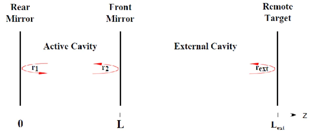
The model in Fig. 1.3 is extended by adding a third external mirror of an effective reflectivity rext at a distance Lext from the front facet to account for
back-reflection from a remote target [109-111]. The three-mirror model is shown in Fig. 1.4.
Fig. 1.4: The three-mirror model of a laser diode subject to optical feedback.
The back-scattered beam may be reflected from the front facet back towards the target in order to theoretically make multiple round trips before re-entering the active cavity [112-114]. This may be used for increasing the accuracy of displacement measurements as the number of fringes is doubled for a given amplitude of displacement. However, we limit our analysis to the case of a single reflection. Also, the models presented in this thesis are limited to the case of the single-mode operation of the laser source.
Assuming a single reflection from the remote target, the electric field at the boundary of the laser external front facet is the sum of the electric field reflected from it and the back-reflected field injected into the laser. This model can be reduced to one similar to that shown in Fig. 1.3 by replacing the external cavity with a single equivalent mirror, as shown in Fig. 1.5, with an electric field reflectivity of req, given by:
1.2 Principles of Optical Feedback Interferometry 15 𝑟eq= 𝑟2 + (1 − |𝑟2|2). 𝑟 ext. 𝑒−𝑗𝜔𝜏ext (1.6) where 𝜏ext = 2 𝐿ext
𝑐 is the round-trip delay time in the external cavity, assuming a
unity refractive index of the external medium.
Fig. 1.5: The reduced model of a laser diode subject to optical feedback. Eq. (1.6) can be rewritten as:
𝑟eq = 𝑟2(1 + 𝜅 𝑒−𝑗𝜔𝜏ext) (1.7)
where κ = (1 − |𝑟2|2) 𝑟ext
𝑟2 is the feedback coupling coefficient, which is a measure
of the coupling strength between the external and active cavities. Eq. (1.7) can be written in a compact complex form:
𝑟eq = |𝑟eq|. 𝑒−𝑗𝜙𝑟 (1.8)
where ϕr is the phase shift of the equivalent reflectivity. In most of the sensing applications, rext is very small compared to r2, and 𝜅 ≪ 1. Hence, the amplitude
and phase shift can be expressed as:
|𝑟eq| = 𝑟2(1 + 𝜅 𝑐𝑜𝑠 (𝜔. 𝜏ext)) (1.9) and
Chapter 1: Principles and Applications of Optical Feedback Interferometry
16
To determine the amplitude and phase under stationary lasing conditions of a laser diode subject to optical feedback, r2 in eq. (1.3) is replaced with req yielding the
amplitude condition:
𝑟1. |𝑟eq|. 𝑒(𝑔−𝛼𝑠)𝐿 = 1 (1.11)
and the phase condition:
4𝜋𝜈𝑛eff𝐿
𝑐 + 𝜙𝑟 = 2𝑚𝜋 (1.12)
Eq.s (1.11) and (1.12) explicitly show that the presence of optical feedback leads to changes in the laser properties such as threshold gain, output power and lasing frequency. The threshold gain under optical feedback, gc, is then expressed as:
𝑔𝑐 = 𝛼𝑠 + 1 𝐿 𝑙𝑛( 1 𝑟1. |𝑟eq| ) (1.13)
Replacing |req| with its equivalent expression in eq. (1.9), and expressing eq.
(1.13) in terms of gth, we obtain: 𝑔𝑐 = 𝑔th−
1
𝐿 𝑙𝑛(1 + 𝜅 𝑐𝑜𝑠 (𝜔. 𝜏ext)) (1.14)
The change in threshold gain due to optical feedback, Δg defined as 𝛥𝑔 = 𝑔𝑐 −
𝑔th, is then expressed as:
𝛥𝑔 = − 𝜅
𝐿 𝑐𝑜𝑠 (𝜔. 𝜏ext) (1.15)
where the linear approximation: ln(1 + 𝑥) ≅ 𝑥 if 𝑥 ≪ 1 is applied as 𝜅 ≪ 1. Clearly, due to optical feedback, the gain changes periodically with the target distance, Lext.
So far, we have demonstrated through equations (1.11) and (1.12) that, due to optical feedback, both threshold gain and emission frequency encounter changes. These changes lead to a change in the effective refractive index of the laser medium as it is a function of both frequency and gain. The gain change influence on the effective refractive index is indirect but occurs through the influence on the
1.2 Principles of Optical Feedback Interferometry
17 carrier density within the laser cavity, N. The effective refractive index, threshold gain and carrier density are linked to each other through the expression [111]:
𝜕𝑛eff
𝜕𝑁 (𝑁 − 𝑁th) = − 𝛼𝑐
4𝜋𝜈th (𝑔 − 𝑔th) (1.16)
where Nth is the threshold carrier and α is the linewidth enhancement factor.
Eq. (1.12) of the phase condition is only satisfied when the round-trip phase within the compound cavity, ϕL, is an integer multiple of 2π. In other words, the round-trip phase change due to optical feedback should be zero to meet the phase condition. The phase change can be expressed as:
𝛥𝜙𝐿 =4𝜋𝛥(𝜈. 𝑛eff)𝐿
𝑐 + 𝜙𝑟 (1.17)
The total change in the product of frequency and effective refractive index due to optical feedback is given by:
𝛥(𝜈. 𝑛eff) = 𝜈th. 𝛥𝑛eff+ 𝑛eff,th. 𝛥𝜈 (1.18) where 𝛥𝜈 = 𝜈 − 𝜈th is the deviation from the lasing frequency of the solitary
laser diode, νth, and 𝛥𝑛eff= 𝑛eff− 𝑛eff,th is the deviation from the effective
refractive index of the active medium within the solitary laser diode, 𝑛eff,th.
In eq. (1.17), the first term on the right hand side rises from the change induced by optical feedback on both the lasing frequency and the effective refractive index. The second term is the phase shift in the external cavity.
The effective refractive index is a function of both frequency and carrier density. Therefore, the change in the effective refractive index can be expressed as [111]:
𝛥𝑛eff = 𝜕𝑛eff
𝜕𝑁 (𝑁 − 𝑁th) + 𝜕𝑛eff
𝜕𝜈 (𝜈 − 𝜈th) (1.19)
Chapter 1: Principles and Applications of Optical Feedback Interferometry 18 𝛥(𝜈. 𝑛eff) = −𝛼𝑐 4𝜋 (𝑔𝑐− 𝑔th) + 𝜈𝑡ℎ 𝜕𝑛eff 𝜕𝜈 (𝜈 − 𝜈th) + 𝑛eff,th(𝜈 − 𝜈th) (1.20)
The effective group refractive index, ng, defined as the ratio of the speed of light in vacuum to the group velocity in the medium, is expressed as [111]:
𝑛𝑔 = 𝑛eff+ 𝜈th
𝜕𝑛eff
𝜕𝜈 (1.21)
Using eq. (1.21), eq. (1.20) can be simplified to: 𝛥(𝜈. 𝑛eff) = −𝛼𝑐
4𝜋 (𝑔𝑐 − 𝑔th) + 𝑛𝑔(𝜈 − 𝜈th) (1.22) Substituting eq. (1.22) into eq. (1.17), the later can be rewritten as:
𝛥𝜑𝐿 = −𝛼𝐿(𝑔𝑐− 𝑔th) +4𝜋𝑛𝑔. 𝐿
𝑐 (𝜈 − 𝜈th) + 𝜑𝑟 (1.23)
Substituting the phase shift in the external cavity from eq. (1.10) and the threshold gain change from eq. (1.15) into eq. (1.23), the round-trip phase change becomes:
𝛥𝜑𝐿 = 4𝜋𝑛𝑔. 𝐿
𝑐 (𝜈 − 𝜈𝑡ℎ) + 𝜅 [sin(𝜔. 𝜏ext) + 𝛼. cos (𝜔. 𝜏ext)] (1.24) which can be expressed in a more compact form:
𝛥𝜑𝐿 = 𝛥𝜔. 𝜏𝐿+ 𝜅√1 + 𝛼2. sin (𝜔. 𝜏
ext+ tan−1𝛼) (1.25)
where Δω is the change in angular lasing frequency due to optical feedback, ωth is
the angular lasing frequency of the solitary laser diode and 𝜏𝐿 = 2 𝑛eff.𝐿
𝑐 is the
round-trip delay time inside the laser cavity.
The lasing frequency of the laser diode subject to optical feedback is determined by setting eq. (1.25) to zero for the phase condition to be satisfied. Thus, the lasing frequency under optical feedback can be expressed as:
1.2 Principles of Optical Feedback Interferometry
19 𝜈 = 𝜈th−
𝐶
2𝜋𝜏extsin (𝜔. 𝜏ext+ tan
−1𝛼) (1.26)
where C is the feedback parameter which is expressed as: 𝐶 =𝜏ext
𝜏𝐿 𝜅√1 + 𝛼2 (1.27)
Eq. (1.27) shows that the dimensionless C parameter depends on the distance to the remote target as well as the quantity of light re-injected into the laser cavity. The stronger is the optical feedback, the higher is C.
1.2.1.3 Optical feedback Regimes
In order to determine the influence of the dimensionless feedback parameter C on the round-trip phase change, and hence the possible solutions of lasing frequencies under optical feedback, we re-express eq. (1.26) as:
𝛥𝜑𝐿 = 2𝜋𝜏ext(𝜈 − 𝜈𝑡ℎ) + 𝐶. sin (𝜔. 𝜏ext+ tan−1𝛼) (1.28)
Fig. 1.6 shows the round-trip phase change simulated using MATLAB and plotted as a function of 𝜈 − 𝜈th for different values of C. The number of possible
solutions of lasing frequencies is determined by the number of the zero-crossings of the round-trip phase change. The standalone laser diode operates at the unperturbed lasing frequency which is determined by the zero-crossing of the linear blue solid line.
In the presence of optical feedback, the zero-crossing, and thus the lasing frequency, is shifted from the threshold frequency. The number of the possible lasing modes depends mainly on the value of the feedback parameter C.
Chapter 1: Principles and Applications of Optical Feedback Interferometry
20
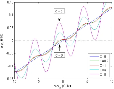
Fig. 1.6: The round-trip phase change against the lasing frequency change simulated for different values of the feedback parameter C.
As indicated in Fig. 1.6, for 𝐶 < 1 which corresponds to weak optical feedback levels, the round-trip phase change increases monotonically with frequency yielding a single zero-crossing. Hence, the round-trip phase change has a single solution, and thus a single-mode operation. Since the purpose of the work presented in this thesis is to evaluate the laser parameters that impact the sensor sensitivity, we have limited our modelling to this range of C values.
For 𝐶 > 1, the feedback is stronger and the round-trip phase is no longer monotonically increasing with frequency, rather it oscillates yielding multiple zero-crossings, which means multiple solutions. If the case of maximum three possible solutions is considered, the maximum value of C that satisfies this condition is calculated by solving eq. (1.28) and found to be 4.6 [115].
Indeed, for the values from 1 < 𝐶 < 4.6, the feedback is considered moderate, and the OFI signal assumes a saw-tooth like shape. The laser becomes bi-stable, and out of the three possible solutions: one is unstable while the other two are stable [116]. Even so, the laser diode still operates in single-mode as only the mode having the narrowest spectral width will be chosen by the laser diode [117-119], with the possibility of mode-hoping occurring.
1.2 Principles of Optical Feedback Interferometry
21 For C > 4.6, the optical feedback level is considered strong and the system theoretically becomes multi-stable with mode-hopping as at least five solutions satisfying eq. (1.28). Very high values of C may lead to coherence collapse where the interferometric measurement is no longer possible.
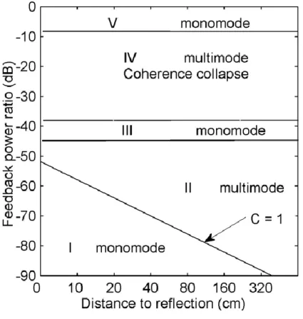
Therefore, the number of the possible solutions of the round-trip phase change equation depends on the value of the feedback parameter C. Based on the number of solutions, the functioning of the laser can be divided into five regimes [120], as shown in Table 1.1 and Fig. 1.7:
Regime I
Weak optical feedback with (the feedback fraction of the amplitude is less than 0.01%). The linewidth of the lasing mode is narrow for weaker feedback levels and broadens with the increase of the feedback level.
Regime II
Moderate optical feedback (the feedback fraction of the amplitude is less than 0.1%). Generation of the external modes leads to mode hopping among internal and external modes.
Regime III
The feedback fraction of the amplitude is around 0.1%. The laser is perfectly single-mode and the spectral width is very narrow. Due to its narrow feedback ratio, this regime is difficult to obtain experimentally.
Regime IV
Strong optical feedback (the feedback fraction of the amplitude is around 1%). This is the coherence collapse regime which often is not appropriate for OFI sensing as the laser diode in this regime loses all its coherence properties and its linewidth is broadened greatly.
Regime V
Very strong optical feedback (the feedback fraction of the amplitude is higher than 10% feedback). The laser comes back to being single-mode with a very high rejection on the lateral modes of the laser cavity and exhibiting a very narrow spectral width. Because of the high instability of the laser diode in this regime, it is more suitable for chaos applications [121].
Chapter 1: Principles and Applications of Optical Feedback Interferometry
22
Fig. 1.7: The regimes of optical feedback levels at different power ratios.
1.3 Applications of Optical Feedback Interferometry
Optical feedback interferometry is a promising sensing technique for both industrial and laboratory environments due to its simple optical setup and cost-effectiveness compared to other interferometric techniques. Typical sensing applications of OFI are the measurement of displacement, absolute distance, vibration and velocity. Each of these applications fathers many sub-domain applications which are well covered by OFI literature, as the number of publications on OFI applications has been rapidly increasing since the early 1990s.
In this section, we briefly discuss the main typical sensing applications as well as two of the most recent OFI sensing applications: particle sizing and detection, and acoustics. We intentionally chose to discuss about those two applications because they all require high sensitivity, which is one of the goals of our work.
1.3 Applications of Optical Feedback Interferometry
23 1.3.1 Typical sensing applications
Here, we present brief introductions of the main sensing applications that are widely covered in literature, namely the measurements of displacement, absolute distance, vibration and velocity.
a) Displacement:
The basic setup used in the measurement of the displacement of a moving target is shown in Fig. 1.8(a). When the target is moving along the optical path, the length of the external cavity is varying and so is the complex electric field reflectivity of the equivalent cavity. Those variations in the complex reflectivity affect the laser properties.
From eq. (1.15), we can see that the change in the gain due to optical feedback is periodic with a period of 𝜙 = 𝜔. 𝜏𝑒𝑥𝑡. Considering a full period swing in gain, we
can evaluate the displacement in terms of wavelength by first evaluating the change in the external round-trip delay time due to displacement:
|𝜔. 𝛥𝜏𝑒𝑥𝑡| = 2𝜋 (1.29)
where 𝛥𝜏𝑒𝑥𝑡 is the change in the external round-trip delay time due to a target
displacement of ΔD. Then, the target displacement due to a full swing can be expressed as:
|𝛥𝐷| =𝜆
2 (1.30)
From eq. (1.30), we deduce that the resolution is in order of half of the operating wavelength. Actually, this resolution could be improved using several technical methods such as: the linearization of the normalized optical power that has been approximated by an ideal sawtooth signal [122], a fast modulation of the optical path difference of an OFI sensor that modifies the round-trip external delay [123], or the use of a pair of laser diodes, each with its own external cavity, where the first laser diode is used as a reference while the other is perturbed by the target displacement [124].
In addition, the resolution could also be improved using several signal processing techniques such as: the phase demodulation or un-wrapping method [125], the use
Chapter 1: Principles and Applications of Optical Feedback Interferometry
24
of extended Kalman filters [126], the use of wavelets transforms [127] or the use of genetic algorithms [128].
(a) Basic representation of the displacement measurement setup.
(b) A sinusoidal displacement with sawtooth-like fluctuations.
Fig. 1.8: The displacement of a target can be retrieved from processing the OFI signal acquired for a target moving along the optical path of a laser diode: (a) basic representation of the displacement measurement setup, and (b) a sinusoidal displacement with sawtooth-like fluctuations.
Fig. 1.8(b) shows a sawtooth-like modulation of an OFI signal corresponding to a sinusoidal displacement. We can observe that the number of sawtooth-like fringes
1.3 Applications of Optical Feedback Interferometry
25 is directly proportional to the displacement. Moreover, the asymmetric shape of the fringes permits to directly recover the target direction of displacement.
By counting the fringes and adding them with their proper sign, we can retrieve the displacement with the basic resolution of λ/2. For example, if N fringes are detected for a motion in one direction, then the corresponding displacement D of the target is given by:
𝐷 = 𝑁 𝜆
2 (1.31)
In comparison to a conventional system, the displacement can be retrieved using only the laser diode and a collimating lens to focus the beam spot on the target surface while conventionally the same information can be retrieved using two interferometric channels.
b) Vibration:
In many mechanical or mechatronic fields, vibration measurement is essentially demanded for the reduction or the elimination of the resultant vibration noise. In addition, it can be used for the quality control of the manufactured products to counter excessive vibration that may damage the product, limit processing speeds, or even cause catastrophic machine failure.
In 1996, Roos et al. first demonstrated the measurement of vibration using a laser diode OFI sensor [129]. Since then, many researchers concentrated their attention on this technique due to the low cost and compactness of the OFI sensor compared to conventional sensors. Other advantages include the high sensitivity, large bandwidth and a large dynamic range up to 70 kHz and 100 dB, respectively [130]. Moreover, it is able to function on different types of surfaces without any optical modulation as well it allows the measurement of low frequency vibrations. For example, the first sensor developed by Roos et al. allowed the measurement of vibrations in approximately all types of surfaces with a bandwidth ranging from 0.1 Hz to 70 KHz and a maximal peak to peak amplitude of 180 μm. A special algorithm was developed in order to analyse the OFI signal in real time which enabled the tracking of the target velocity variations.
Chapter 1: Principles and Applications of Optical Feedback Interferometry
26
In 2004, Scalise et al. used a laser diode OFI vibrometer in piezoelectric transducers characterization which measured both the velocities as well as the vibrations of solid targets with results comparable to those obtained by the conventional LDV by deploying a technique similar to the one used in LDV allowing the processing of the OFI signals even in the presence of speckle [69]. A more recent recovery technique of signals in an OFI vibrometer has been published in 2008 where the single beat frequency is extracted over a period containing a few fringes at least [131]. This method has allowed to rectify the problems of speckle, electromagnetic interference and mechanically induced parasitic signal fluctuations for an ultrasound solder vibrating at 20 kHz with an amplitude of 40μm.
c) Velocity:
The measurement of velocity is essentially desired in many areas like aerospace, automotive, metallurgy and paper industry, with an increasing demand for remote sensing of rough targets in hostile environments and in in-line assembly processes. Many techniques are used for the velocity measurements but either they have poor spatial definition like in ultrasonic sensors or they are expensive like in Laser Doppler Velocimetry (LDV). OFI sensors have the advantages of compactness, low cost and compatibility.
The main principle of this technique is based on Doppler-Fizeau effect. In the case of OFI velocimetry, either the laser diode or the remote target is static while the other is moving relatively. The Doppler frequency FD that corresponds to the frequency of the sawtooth-like OFI signal can be expressed in terms of the velocity of the target VF as:
𝐹𝐷 = 2𝑉𝐹
𝜆 (1.32)
Even when a target moves in a direction other than the propagation direction, the OFI sensor can still be used to measure the velocity of the target. In this case, we account for the angle that the direction of movement makes with the optical axis
1.3 Applications of Optical Feedback Interferometry
27 𝐹𝐷 =
2𝑉𝐹
𝜆 𝑐𝑜𝑠 (Ɵ) (1.33)
An example of a measurement setup of rotating tilted targets is shown in Fig. 1.9(a) whereas Fig. 1.9(b) depicts an example of the electrical spectrum of the OFI velocimetric signal acquired for this setup.
(a) Basic representation of the velocity measurement setup.
(b) Example of an OFI signal spectrum.
Fig. 1.9: Laser Doppler velocimetry demonstration with a VCSEL sensor: a) basic representation of the velocity measurement setup, and b) an OFI signal spectrum.
Chapter 1: Principles and Applications of Optical Feedback Interferometry
28
Recently, an on-board double-laser diode velocity sensor has been successfully tested by removing the influence of the pitching and the pumping effects in order to improve both the accuracy and the robustness of the OFI velocimetry system [132]. Furthermore, in order to improve the OFI velocimeter resolution by a factor of 10 when the Doppler frequency measurement was strongly affected by the roughness of the target surface, a second order auto-regressive algorithm has also been applied to the OFI signal [133]. In 2008, an OFI velocimeter based on a commercial 850nm VCSEL has been used for the measurement of velocity by acquiring and processing the LV OFI signal [107]. The velocimetry principle is also used for the measurement of flow rates in fluidics.
d) Absolute distance:
OFI sensors can also be used as range finder techniques besides the geometric technique of triangulation and the time-of-flight (TOF) technique [134]. The geometric technique of triangulation is widely used in industrial applications due to its low cost and robustness, yet it lacks the auto-alignment and has a limited distance-dependent sensitivity. The TOF technique, on the other hand, provides a long distance measurement coverage up to tens of kilometres with a uniform sensitivity throughout the whole measurement range, yet they are not the most accurate. The most accurate but very expensive approach is the interferometric technique which is mostly used in metrology when high accuracy is demanded. On the other hand, OFI sensors offer a low-cost and compact alternate solution.
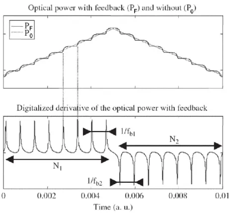
In this configuration, the external cavity length is constant while the length of the active cavity is varying due to the continuous modulation of the laser injection current. As shown in Fig. 1.10, a properly shaped triangular waveform is used for the modulation of the current in order to enable the measurement of the absolute distance, inducing a triangular variation of Δλ in the operating wavelength, corresponding to a variation of (-2πΔλ/λ2) in the wave number.
Variations of the output optical power PF under optical feedback will then be superimposed on the output optical power of the solitary laser diode P0 which corresponds to the triangular carrier as depicted in Fig. 1.10. By performing a
1.3 Applications of Optical Feedback Interferometry
29 derivative of this OFI signal, characteristic spikes can be retrieved and digitalized for further signal processing to calculate the distance.
Fig. 1.10: Optical power variations and their corresponding beat frequencies for a triangular injection current.
The distance D was initially calculated by counting the integer number of those spikes. In more details, let us consider N1 and N2 as the number of spikes recorded during the increasing and decreasing triangular semi-period respectively as well as
N as their sum in a complete period TP of the modulating triangular signal. Then the distance can be approximately expressed as [135]:
𝐷 ≈ 𝜆
2
2∆𝜆𝑁 ≃ 𝑐
2∆𝜈𝑁 (1.34)
where Δν the optical frequency shift.
The accuracy can be improved by determining the beat frequencies fb,1 and fb,2 between the spikes of the upward and downward triangular signal respectively, yielding the following exact relationship [109]:
![Fig. 1.11: A schematic diagram of the of the acoustic filed measurement setup [139].](https://thumb-eu.123doks.com/thumbv2/123doknet/3108719.88246/45.892.192.746.99.451/fig-schematic-diagram-acoustic-filed-measurement-setup.webp)
![Fig. 1.12: Propagation of the acoustic field with the ultrasonic transmitter propagating the field into free space; Left: measured, Right: simulation [139]](https://thumb-eu.123doks.com/thumbv2/123doknet/3108719.88246/46.892.156.698.120.393/propagation-acoustic-ultrasonic-transmitter-propagating-measured-right-simulation.webp)
![Fig. 1.13: Experimental setup for edge filter enhanced self-mixing interferometry (ESMI) experiments [145]](https://thumb-eu.123doks.com/thumbv2/123doknet/3108719.88246/47.892.230.709.530.784/experimental-setup-filter-enhanced-mixing-interferometry-esmi-experiments.webp)