Photo-Acoustic Tomography (PAT) based on Laser Optical Feedback Imaging (LOFI) of surface displacements

HAL Id: hal-02282968

https://hal.archives-ouvertes.fr/hal-02282968

Submitted on 10 Sep 2019

HAL is a multi-disciplinary open access

archive for the deposit and dissemination of

sci-entific research documents, whether they are

pub-lished or not. The documents may come from

teaching and research institutions in France or

abroad, or from public or private research centers.

L’archive ouverte pluridisciplinaire HAL, est

destinée au dépôt et à la diffusion de documents

scientifiques de niveau recherche, publiés ou non,

émanant des établissements d’enseignement et de

recherche français ou étrangers, des laboratoires

publics ou privés.

Photo-Acoustic Tomography (PAT) based on Laser

Optical Feedback Imaging (LOFI) of surface

displacements

Vadim Girardeau, Olivier Jacquin, Olivier Hugon, Bathilde Riviere,

Boudewijn van der Sanden, Eric Lacot

To cite this version:

Vadim Girardeau, Olivier Jacquin, Olivier Hugon, Bathilde Riviere, Boudewijn van der Sanden,

et al.. Photo-Acoustic Tomography (PAT) based on Laser Optical Feedback Imaging (LOFI) of

surface displacements. Applied optics, Optical Society of America, 2019, 58 (26), pp.7195-7204.

�10.1364/AO.58.007195�. �hal-02282968�

HAL Id: hal-02282968

https://hal.archives-ouvertes.fr/hal-02282968

Submitted on 10 Sep 2019

HAL is a multi-disciplinary open access

archive for the deposit and dissemination of

sci-entific research documents, whether they are

pub-lished or not. The documents may come from

teaching and research institutions in France or

abroad, or from public or private research centers.

L’archive ouverte pluridisciplinaire HAL, est

destinée au dépôt et à la diffusion de documents

scientifiques de niveau recherche, publiés ou non,

émanant des établissements d’enseignement et de

recherche français ou étrangers, des laboratoires

publics ou privés.

Photo-acoustic tomography based on laser optical

feedback imaging of surface displacements

Vadim Girardeau, Olivier Jacquin, Olivier Hugon, Bathilde Riviere,

Boudewijn van der Sanden, Eric Lacot

To cite this version:

Vadim Girardeau, Olivier Jacquin, Olivier Hugon, Bathilde Riviere, Boudewijn van der Sanden, et al..

Photo-acoustic tomography based on laser optical feedback imaging of surface displacements. Applied

optics, Optical Society of America, 2019, 58 (26), pp.7195. �10.1364/AO.58.007195�. �hal-02282968�

Photo-Acoustic Tomography (PAT) based on Laser

Optical Feedback Imaging (LOFI) of surface

displacements

V

ADIM

G

IRARDEAU

,

1

O

LIVIER

J

ACQUIN

,

1

O

LIVIER

H

UGON

,

1

B

ATHILDE

R

IVIERE

1

B

OUDEWIJN VAN DER

S

ANDEN

,

2

AND

E

RIC

L

ACOT

1,*

1

Univ. Grenoble Alpes, CNRS, LIPhy, F-38000 Grenoble, France 2

Univ. Grenoble Alpes, INSERM, CNRS, TIMC-IMAG, F-38000 Grenoble, France * _{Corresponding author: eric.lacot@univ-grenoble-alpes.fr}

Received XX Month XXXX; revised XX Month, XXXX; accepted XX Month XXXX; posted XX Month XXXX (Doc. ID XXXXX); published XX Month XXXX

We present how a Laser Optical Feedback Imaging (LOFI) setup can be used for the optical detection of ultrasound in Photo-Acoustic Tomography (PAT). A PAT image is reconstructed by an inversion algorithm using surface displacement measurements made at several locations with our LOFI setup and following the optical irradiation with a pulsed Nd:YAG laser of a sample with absorbing inclusions. The width of the reconstructed inclusions and the SNR of the reconstructed images are firstly studied on the numerical model of a sample with 3 absorbing inclusions (i.e. with 3 acoustic punctual sources). Finally an experimental PAT image of a phantom composed of two polyamide tubes with an internal diameter of 800 µm filled with red ink and submerged at -3.5 mm depth in a tank filled with water is reconstructed. Experimentally, the water surface displacement measurements has been made with our LOFI vibrometer which provides an amplitude sensitivity of 1nm (for a single-shot measurement) in a detection bandwidth of roughly 1 MHz adapted to the detection of the polyamide tubes. Under our experimental conditions, the surface energy densities, of the LOFI focalized beam for the detection and of the pulsed Nd:YAG laser used for the irradiation, are compatible with the MPE (Maximum Permissive Exposure) for future biomedical measurements. The SNR and the resolution of the reconstructed PAT images are in good agreement with the theoretical predictions.

http://dx.doi.org/10.1364/AO.99.099999

1. INTRODUCTION

Photo-Acoustic (PA) imaging, which is based on the generation of an acoustic wave from an absorbing object being illuminated by a pulsed or a modulated laser, is a very interesting tool [1-5] in biomedical application. Indeed, PA imaging allows to combine the main advantages of the optical and ultrasound imaging methods, which are the high endogenous (or exogenous) optical absorption contrast in heterogeneous tissues and the low diffusion and absorption of ultrasound waves ( 1 1

1

dB cm MHz

.



.

 ) in the human body [6]. Whatever the imaging mode: OR-PAM (Optical Resolution Photo-Acoustic Microscopy), AR-PAM (Photo-Acoustic Resolution Photo-Photo-Acoustic Microscopy) or PAT (Photo-Acoustic Tomography), PA Imaging provides highly contrasted images with a ratio between the transversal resolution and the penetration depth roughly equals to 1/100, e.g.: a resolution of 100 µm at 1cm depth or of 1µm à 100µm depth) [7]. This

is the average limit of several medical imaging techniques, such as MRI, CT and ultrasound. As mentioned in [8], piezoelectric transducers (PZT) are commonly used to detect laser-induced ultrasonic waves in PA imaging. However, they typically lack adequate broadband sensitivity at high ultrasonic frequency (i.e. at high resolution) whereas their bulky size and optically opaque nature cause technical difficulties in integrating PA imaging with conventional optical imaging modalities. To overcome these limitations, optical methods of ultrasound detection were developed and shown their unique applications in PA imaging. We have [8]: the free-space optics based ultrasound detection (Michelson and Mach Zehnder interferometers), The fiber optics based ultrasound detection (fiber optics interferometer, single fiber sensor with Bragg grating or with Fabry Perrot cavity), the photonic integrated circuit detectors (polymer optical waveguide sensor, micro-cavity resonators) and the ultrasound detection via optical interface (Fresnel reflection, photonic crystal cavity, surface plasmon resonance, Metamaterials).

The main objective of the present paper is to demonstrate how a Laser Optical Feedback Imaging (LOFI) setup (which is an optical free space technic [8]) can be used for optical detection of ultrasound in Photo-Acoustic Tomography (PAT). Nanometer measurements based on SMI (Self Mixing Interferometry) have already been realized, either for acoustic perturbations or for nm-sized vibrations [9-14]. Here, the use of a LOFI setup is motivated by the combination of the four following reasons: i) The LOFI interferometer is always self-aligned because the laser simultaneously fulfils the functions of the source (i.e. photons-emitter) and of the photo-detector (i.e. photons-receptor); ii) The phase of the interferometric signal (i.e. of the LOFI beating) is sensitive to the round-trip distance between the laser and the vibrating target. iii) The LOFI sensitivity allows analysis of targets with a weak back-reflected (or back-scattered) electric field. iv) The LOFI detection is shot noise limited (even with a low power laser and a conventional detection) in a frequency range located near the relaxation oscillation frequency of the laser [15-16]. Therefore, the LOFI setup can respect medical conditions: security and easy to integrate.

This paper is organized as follows. In the first section, the principle of the acquisition of PA signal with a LOFI set-up is explained. The next section deals with principle of the image reconstruction from the surface displacement measurements. The point spread function (PSF) and the signal to noise ratio (SNR) of the reconstructed images are studied. Analytical predictions are compared with the results of a numerical simulations performed on 3 punctual acoustic sources immersed in water. Finally, an in depth experimental image reconstruction obtained from the LOFI signal is shown, where the absorbing sample, illuminated by a green pulsed laser, is a phantom composed of two polyamide tubes filled with red ink and submerged at -3.5 mm depth in a tank filled with water. The final section is a general discussion of these results and possible applications in in vivo Photo-Acoustic (PA) imaging.

2. PRINCIPLE OF THE SIGNAL ACQUISITION

A schematic diagram of the Photo-Acoustic Tomography (PAT) based on Laser Optical Feedback Imaging (LOFI) is shown in Fig. 1. Experimentally, the Photo-Acoustic (PA) effect is generated by a frequency doubled Nd:YAG laser (532 nm) with a pulsed width:

10 L ns



  and a repetition rate of 10 Hz . The laser light is send on absorbing inclusions characterized by the absorption coefficient

1

a cm

 _  _{and immersed at several millimeters depth in a tank filed}

with water. After a time delay (linked to the sound velocity in water

1500 a

c  m s), the transient pressure waves generated by the

thermal expansion of the absorbing medium reach the air/water interface (i.e. the plane z0mm), which is then transiently

displaced of a few nanometers.

To measure the time resolved surface displacement (induced by the PA effect), we have used a LOFI (Laser Optical Feedback Imaging) interferometer, which is a very sensitive heterodyne interferometer involving the laser dynamics [15-16]. In this imaging system, an optical beating occurs inside the laser cavity, between the intra-cavity light and the light backscattered by the target. By this way, the laser is the source and also the detector, which implies that it is very easy to use (this optical system is self-aligned) and the measures are “shot-noise” limited. The LOFI laser is a CW Nd:YAG microchip laser with a maximum available power of several mW at a wavelength of

1064

L nm



 and a relaxation oscillation frequency F_R in the

megahertz range. The microchip laser beam is focused on the

air/water interface and part of the light reflected and/or scattered by the moving interface returns inside the laser cavity after a second pass through the frequency shifter. Therefore, the optical frequencies of the reinjected light are shifted by F_e. This frequency shift can be adjusted

and is typically of the order of the laser relaxation oscillation frequency

R

F to obtain a shot noise limited signal [15-16]. The microchip laser

cavity is relatively short (typically 1mm ) which ensures a high damping rate of the laser cavity (typically



10 s

9 1) and therefore a good sensitivity to weak optical feedback [15,16].

For a given position



x y,



of the laser focalizing spot on the water

surface (i.e. the planez0), and in the case of weak optical

reinjection, the coherent interaction (beating) between the lasing electric field and the frequency-shifted reinjected field leads to a sinusoidal modulation of the laser output power. For detection purposes, a small part of the laser output beam is sent to a photodiode. The delivered voltage is processed by a PC to finally obtain a quantitative measurement of the small local displacement of the air/water interface: da



x y t, ,







L[14]. Experimentally, a LOFI

movie of the surface displacement can be obtained pixel by pixel (i.e. point by point, line after line) by a full 2D galvanometric scanning of the microchip laser focal spot on the air/water interface or by a displacement of the absorbing target by using a motorized translation stage. Each LOFI punctual measurements is triggered on the optical irradiation of the sample by the pulsed Nd:YAG laser.

Fig. 1. Schematic diagram of PAT based on a LOFI setup. PA Laser:

Laser with a pulse width 



_L for PA generation; Target: Two parallel polyamide tubes filled with ink with an absorption coefficient

 

1

a

cm



 _{; µLaser: microchip laser, with a relaxation oscillations}

frequency FR, for LOFI measurement of surface displacements. L1, L2, L3 and L4: Lenses, BS: Beam Splitter, PD: Photodiode, FS Frequency Shifter with a round trip frequency-shift F_e GS: Galvanometric

Scanner, MTS: Motorized translation stages.

3. PRINCIPLE OF THE IMAGE RECONTRUCTION

A. Image reconstruction algorithm

The image reconstruction algorithm is firstly studied on a numerical example. Fig. 2 shows the reconstruction of four 2D images obtained from the simulation of the surface temporal displacements induced by

max 3

j  acoustic waves. For an easier comparison of the different

images, the size of the reconstruction widows is always the same. In this numerical example, the acoustic sources are immersed in water and located on a vertical line perpendicular to the water surface and

the time evolution of the surface displacement is obtained at

max 11

i  distinct locations on the water surface.

In the present numerical simulation, the time evolution of the surface displacement at the detection locations (X_{d i,},Y_{d i,} ,Z_{d i,} 0) with i_1, 2,...,i_max_is given by:

 









, , max , , , , , , 1

,

,

i a d i d i n j s j s j s j i j s j i j j

d t

d

X

Y

t

S

A

P

t

r















_



_











, (1)

where for the acoustic source labeledj_1, 2,...,j_max_, As j, is the

displacement amplitude at the source location, while S_{s j,} is the

characteristic surface of the source.



 

2

 

2



2

, , , , , , ,

i j d i s j d i s j d i s j

r



X



X



Y



Y



Z



Z

is the

geometrical distance between the i_th detection location (X_{d i,} ,Y_{d i,} ,

,

d i

Z ) and the

j

_th source location (X_{s j,} ,Y_{s j,} ,Z_{s j,} ), while , , i j i j a

r

c





is the corresponding time delay for an acoustic wave propagating with a velocity of ca1500m s in water. In Eq. (1), the

exponent

n

allows to describe different types of acoustic wave:

0

n



for plane waves;

n



0.5

for cylindrical waves;

n



1

for spherical waves. Always in Eq. (1), the dimensionless temporal profile of the acoustic wave is given by:

 

2 , , exp 2 s j s j t P t



 _{ }     _ _ _{ }   _{ }    ,

where





_{s j,} is the time width of the detected acoustic signal generated by the photo-acoustic effect with the corresponding wavelength



_{s j,}

 

c

_a



_{s j,} . Due to a convolution effect, one have:

2 2 2

, ,

s j L a j d











   

 

, where





Lis the pulse width of

the PA laser,





_{a j,} are the time width of the emitted acoustic waves and





_d is the time response of the detection which corresponds to a detection bandwidth of:



F

d

 

1



d.

In our numerical simulation the following simplification has been used:

i/ The 3 sources have the same size (S_{s j,} S_a), and emit spherical

waves (

n



1

) with the same amplitude (A_{s j,} A_a).

ii/ For the photoacoustic point of view, we have supposed that not only the thermal diffusion, but also the volume expansion of the absorber during the laser illumination period is negligible. This condition is referred to as the acoustic stress confinement







a j,  



L



) [1-2]. To study the Point Spread Function (PSF)

of the reconstructed image with our PAT setup,, the acoustic sources need to be considered as being punctual sources







_d  



_{a j,}



. Under these conditions the acoustic signal wavelength is given by:

s

c

a



d

c

a

F

d

  





.

iii/ To be in agreement with the PAT-LOFI experimental results shown in the section 4, the following boundary condition has been used to describe the maximum detected amplitude for the water surface displacement:

 

, 10 min a a i j Z A nm r  , (2)

where

Z

_a



S

_a



_sis the acoustic Rayleigh range.

To reconstruct the image I_s



x y z, ,



of the acoustic sources from

the displacement measurementsd t_i

 

, the inversion (i.e. the back

projection) algorithm which has been used is the one used in [17]:





max



 



max 1

1

, ,

, ,

, ,

i s i i i i

I

x y z

d

x y z W x y z

i

_











_

_

(3a)







, ,



, , n i i ref r x y z W x y z r          (3b) where:











 

2

 

2



2 , , ,

, ,

, ,

i i a d i d i d i a

r x y z

x y z

c

X

x

Y

y

Z

z

c

















is the

time delay for the acoustic propagation between the

i

_th detection locations (X_{d i,},Y_{d i,} ,Z_{d i,} ) and the spatial position



x y z, ,



where

the image is reconstructed. In Eq. (3a), the summation is made over the i_max measurement locations. In Eq. (3b), W x y zi



, ,



is the

dimensionless weighting factor which compensates here the attenuation of the acoustics waves due to the propagation from the acoustics sources to the detection location. r_ref is a normalization

distance which can be chosen arbitrary. Indeed this term is simply a multiplicative constant for the whole reconstructed image. In our numerical simulation, for the simplicity of our analytical calculations, we have chosen: r_ref Z_a.

The maximum size of the reconstructed images is not only linked to the detection positions, but is given by the condition:



, ,



max

i x y z T



 , where

T

_maxis the duration of the temporal

acquisition of the surface displacement d t_i

 

. Also, the possible

minimum pixel size is linked to the laser pulse width:

c

a





L.

As explained by Carp et al in [17], the image reconstruction given by Eqs. (3a) and (3b) takes advantages of the direct proportionality between the time of arrival of an acoustics signal at a measurement location and the distance between this location and the point of origin of the signal. As depicted in Figs. 2(a) and 2(b), if a large number of detections contain prominent displacement features corresponding to a certain pixel position, the image reconstruction algorithm assigns high source strength to that pixel. Indeed, on each image of Fig. 2, one can observed 3 bright spots corresponding to the reconstruction of the position of the 3 acoustic sources.

However, even for pixels that contain no acoustic sources, their corresponding time windows in the individual traces will contain a displacement feature if acoustic sources lying elsewhere in the sample are equidistant from the detection position. Thus, even “empty” pixel will be assigned a small non- zero acoustic source intensity. This “ghost” acoustic source is the reason why “arcing” artifacts are seen in images reconstructed using simple back-projection algorithms. To mitigate this issue we have use the Coherence Filtering (CF) introduced by Liao et al in [18] and also used in [17]:



, ,





, ,

 

, ,



CF s I x y z I x y z CF x y z (4a)







 





 









 



max max max 2 1 2 max 1 2 max 2 1

, ,

, ,

, ,

, ,

, ,

, ,

, ,

, ,

i i i i i i i i i i s i i i i i

d

x y z W x y z

CF x y z

i

d

x y z W x y z

i

I

x y z

d

x y z W x y z







  











_

_

















_



_













_



_













(4b)

Fig. 2. 2D image reconstructions performed on 3 punctual acoustic

sources located on a vertical line below the water surface (i.e.

0

z



mm

) :

Z

_s,1

 

2

mm

, Zs,2 5mm and

Z

s,3

 

8

mm

. The

reconstruction is obtained from the surface displacements (induced by the pressure of the acoustic waves) measured at 11 distinct lateral positions

i

d

X

along a line segment on the water surface. Left column (a,c): Images reconstructed whenX_{d i,}  



2mm, 2mm



with an

increment of

0.4 mm

. Right column (b, d): Images reconstructed whenX_{d i,}  



10mm,10mm



with an increment of

2 mm

. Top row (a, b): Images reconstructed without the coherence filtering:



, 0,



S

I x y z . Bottom row (c, d): Images reconstructed with the

coherent filtering:I_CF



x y, 0,z



.

As we can see in Figs. 2(c) and 2(d), the multiplication of I_s



x y z, ,



by CF x y z



, ,



reduces the acoustic source intensity assigned to

location



x y z, ,



by Eqs. (3a) and (3b), if the location does not

contain a real acoustic source. Indeed, if at the location



x y z, ,



, the

reconstructed average intensity corresponds the intersection of

max

mi circles, ones obtains:

, max s m a

m

I

A

i



, (5a) max m

m

CF

i



, (5b) 2 , , max CF m s m m a

m

I

I

CF

A

i







 







. (5c) Therefore, the ratio between the reconstructed intensities of a real acoustic source



m

_real



i

_max



and of a ghost source



m

ghost



i

max



is increased by taking into account the coherence

factor: max max max

2

, _{max max} , ,

, ghost , ghost , ghost

CF i s i s i CF m ghost ghost s m s m

I

i

i

I

I

I

m

m

I

I









_



_









. The

final result is a reduction in arcing artifacts and an improvement of the contrast of the reconstructed image.

B. PSF of the reconstructed images

In Fig. 2, the left and right columns show, for the same number (

max 11

j  ) of detection locations, the influence of the size of the

detection zone on the dimensions of the PSF (i.e. the area of each reconstructed sources).

As we can see, the PSF area is defined by the intersection of the circles (more precisely the rings of thickness_s) which allows reconstructing the punctual sources from the back-projection of the temporal displacement measurements. More precisely, our 2D numerical simulation is made with j_max 3 punctual sources

aligned vertically below the water surface: Z_s,1 2mm,

,2 5

s

Z   mm, Z_s,3 8mm, with

X

s j,



0

mm

and

,

0

s j

Y



mm

for all the sources locations. The detection of the displacement induced by the acoustic waves is made at i_max 11

positions along a horizontal X line:

, d d i d X X X     , Y_{d i,} 0mm, Z_{d i,} 0mm, (6) where max , 11 ,1

2X_d  X_{d i } X_d is the length of the detection

segment.

For the reconstructed images shown in the left column [Figs. 2(a) and 2(c)] the detection has been made with 2Xd 4mm while for the

right column images [Figs. 2(b) and 2(d)] the detection has been made with 2X_d 20mm.

In our numerical simulation, in order to be in agreement with our experimental conditions (see section 4), the surface displacement

 

i

d t is calculated for:

0

µs

 

t

T

max



100

µs

. Under this

condition, the reconstruction of the image is roughly possible in a disk with a radius of 2 2

max 15

a

R x z c T  cm centered on the

central detection position (Xd 0,Zd 0). Therefore, a square

image with a length side of 15cm 210cm can be reconstructed.

For an easier comparison of the PSF of the different images, we have chosen to show the reconstruction images in windows with the same size, whatever the detection segment size.

From the size of the detection segment, we define empirically the “mean” synthetic numerical aperture, for a given source depth

 

Z_s

by:

 





2 2 2 2 d s d s X NA Z X Z     (7)

By using Eq. (7), the lateral and in-depth PSFs (



_X,



_Z) of the reconstructed source can be defined and are respectively given by:

 

_{ }

s X s s

Z

NA Z







(8a),

 

 

2

1

s Z s s

Z

NA

Z









(8b)

where  _s c_a



_d 150µm the characteristic wavelength of the

detected acoustic pulse (which corresponds to a detection bandwidth

10 d

F MHz

  ). Finally, by using Eqs. (8a) and (8b) the analytic expression of the reconstructed image obtained from Eq. (3a) is equal to:





 

 

max 2 2 , 1 , 0, exp 2 s j s j X Z j I x y z z Z x z z





    _{    }  _ _{   }         _    _  



(9)

where the Gaussian shape of the reconstructed sources come from the Gaussian shape of the of acoustic signal temporal profile [see Eq. (1)] In agreement with Eqs. (7), (8a) and (8b), one can observe on Fig. 2 how the lateral width of the PSF (



_X) is smaller when the numerical aperture (

NA

) increases (i.e. when X_d increases or when

s

Z decreases), while an opposite evolution occurs for the

in-depth width of the PSF (



_Z). Indeed,



_Z is larger, when the detection zone is larger (i.e. when X_d increases) or when the

depth is smaller (Z_s decreases).

The best compromise between the lateral and in-depth width is obtain for 1

2

NA (i.e. for: X_d 2Z_s) and under this condition, one

obtains:

2 212

X Z s µm







   . (10)

C. Signal to Noise Ratio (SNR) of the reconstructed image

The image reconstruction shown in Fig. 2 has been obtained from a simulated signal with an additive noise. Indeed, for each displacement

 

i

d t a noise d ti

 

has been added with an average and a

standard deviation which are respectively given by:

 

0

i

d t

nm





(11a)

 

2 1 i d t d nm     (11b)

In agreement with the measurements made with our LOFI setup, the noise is therefore independent of the detection position (i.e. independent of the index i) and its amplitude is in the nanometer range for a single shot measurement (see section 4).

For a given detection position



X_d,Y_d 0,Z_d 0



, the signal to

noise ratio (SNR_d) of the interface displacement measurements is

defined by the ratio between the maximum value of the time evolution of the measured displacement and the displacement ground noise:



,



max

 

2 2 a a d s d d s Z A d t X Z SNR X Z d d          (12)

Due to the attenuation of the acoustics waves with the propagation distance the SNR given by Eq. (12) is inversely proportional to the distance between the source location



X_s 0,Y_s 0,Z_s



and the

detection location.

Under our modeling conditions, the maximum and minimum values of

d

SNR are respectively given by:







,1



max

SNR

_d



SNR

_d

0,

Z

_s



10

(13a)







,3



min

SNR

_d



SNR

_d



X

_d

 

10

mm Z

,

_s



1.6

. (13b)

Eq. (13a) corresponds to the maximum value of SNR_dobtained when

the detection distance is minimum. While Eq. (13b), corresponds to the minimum value of SNR_dobtained when the detection distance is

maximum.

More generally, for a given source depth

 

Z_s , an intermediate value

of SNR_d is obtain for an intermediate detection distance, which

corresponds to the detection position localized between the center and one of the edges of the detection segment in our numerical simulation:

 





,int ,1 2 2 , 2 10 2 d d s d d s s s d X SNR Z SNR X Z Z Z X     _   _       (14)

For the situation where the image will be restored with the best compromise between the lateral and in-depth resolutions (i.e. when

,2

2 10

2

s d

Z

 

X



mm

), one obtains:





,1 ,int ,2 ,2 10 2 3 2 s d S d s Z SNR Z X Z       . (15)

In the rest of this section, our goal is to link the in-depth value of the SNR of the reconstructed image

 

CF

I s

SNR

Z

to the intermediate value of signal to noise ratio of the displacement measurement (i.e.

 

,int

d s

SNR Z ).

For the reconstructed source subscripted j, the signal and the variance obtain from Eqs. (3a) and (3b) are respectively given :





max , , , , , max 1 ,

1

,

,

i i j a s j s s j s j s j a a i j a i

r

Z

I

I

X

Y

Z

A

A

i

_

r

Z









(16a)





max 2 2 2 2 , , 2 2 , _{2 2 2} max max 1

2

1

i i j d s j s j a a i

r

_d

X

Z

I

d

i

i

_

Z

Z



_

_





_

_



















(16b)

where for simplicity, we have approximate all the distances

r

_{i j,} by the intermediate distance





2 2

, 2 ,

i j d s j

r  X Z . Finally the SNR of one reconstructed source is given by

 

_{ }





 

max 2 2 max ,int 2 s s a a I S s s d s d s i I A Z SNR Z I Z _{X Z} d i SNR Z    _{ }   (17)

The SNR increase, given by

i

_max , comes from the average of displacement measurements with white noise.

If the coherence factor is taken into account, one finally obtains (see Eqs (4a), (4b) and (5) with m_gosti_max for the signal and mgost 1

for the noise):

CF s I I (18a), max

3

CF s

I

I

i







(18b) and finally:

 

_{ }

max3 2

 

,int

3

CF CF I s d s CF s

I

i

SNR

Z

SNR

Z

I

Z







(19)

Even if the calculation details are not shown here, Eq. (18b) is an approximate formula which can be obtain from a noise propagation calculation. Indeed, starting from the displacement noise (d), one

can obtained after straightforward but tedious derivative calculations the noises



I

s(see Eq. (16b) and



I

CFaccording to d, and finally

Eq. (18b) by keeping only the dominant contribution. The validity of this equation has been checked numerically for different numerical conditions corresponding to potential experimental conditions. Roughly speaking, in Eq. (18b) (and consequently in Eq. (19)), the multiplicative factor 3 and comes from the fact that 3

CF s

I I [see

Eqs. (4a) and (4b)], and the division by i_maxcomes from the coherence

factor which induces for the random noise, the same attenuation than the one for the arcing effect with: mgost 1.

In the following of this manuscript, the goal is to check the analytical expressions of the widths [given by Eqs. (8a) and (8b)] and of the signal to noise ratio [given by Eq. (19)], of the reconstructed acoustic sources, firstly obtained with numerical simulations (Figs. 2 and 3) and secondly obtained with our experimental results (Fig. 4).

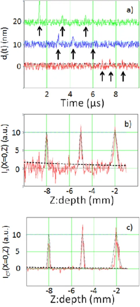
Fig. 3(a) shows 3surface displacements (among the 11) induced by the acoustic waves emitted by the 3 punctual sources. For each displacement simulated, one can observe the arrival times of the acoustic impulsions emitted by the 3 sources located at different depths:

Z

_s,1

 

2

mm

,

Z

_s,2

 

5

mm

and

Z

_s,3

 

8

mm

below the sample surface (i.e.

z



0

mm

). Due to the acoustic wave attenuation with the propagation distance, the displacement amplitude decreases with the arrival time

 

_{i j,}

r

_{i j,}

c

_a . In agreement with Eqs. (13a) and (13b) the signal to noise ratio of the first displacement pulse is maximum and equals to max(SNR_d)10 1 while it is minimum





min

SNR

_d

 

2 1

for the latest one. While for the second peak of the middle trace the SNR is roughly equal to:,

 

,int ,2

3 1

d s

SNR

Z

 

.

Figs. 3(b) and 3(c), show the in-depth reconstruction of the acoustic sources positions obtained respectively without the coherence filtering (I_s



x0,z



) and with the coherence filteringI_CF



x0,z



. One

can notice that Figs. 3(b) and 3(c) correspond respectively to the central vertical line of the images of Figs. 2(b) and 2(d). In agreement with Eq. (8b), the two figures clearly show that that the in-depth width of the reconstructed image (



_Z

 

Z ) decreases with the depth. We

further observed that the weighting factor allows to restore the amplitudes of the wave emitted by the acoustic sources (which are the same in our numerical simulation:A_{S j,} A_a), counterbalanced by an

increase of the in-depth noise.

Regarding the noise, the comparison of Figs. 3(b) and 3(c) clearly shows that the coherence factor reduces the noise level and therefore increases the contrast of the reconstructed sources. In agreement with Eqs. (17) and (19), the signal to noise ratio of the reconstructed central acoustic source is:

3 11 10

s I

SNR





and 3 2

11

3

36

3

CF I

SNR





.

Fig. 3. a) Displacement measurements d t_i

 

induced by the 3

punctual acoustic sources located at:

Z

_s,1

 

2

mm

, Z_s,2 5mm

and

Z

_s,3

 

8

mm

below the water surface with

X

_{s j,}



0

mm

. Lower trace: d t₁

 

measured at

X

d,1

 

X

d

 

10

mm

; Middle

trace: d₄

 

t measured at

X

_d,4

 

4

mm

; Upper trace: d₆

 

t

measured at

X

_d,6



0

mm

. For clarity the different measurements are vertically shifted by a 10 nanometer step. For each displacement measurement, the 3 black arrows indicate the arrival times of the acoustic impulsions emitted by the 3 sources and the horizontal dashed-line is the displacement noise level

 

d

1

nm

. b) In depth reconstruction of the acoustic sources positions obtained without the coherence filtering: IS



x0,z



. The dashed line is the noise level

given by Eq. (16b).The dotted line is the in-depth reconstructed signal given by the analytical expression of Eq. (9). c) In depth reconstruction of the acoustic source position obtained with the coherence filtering:



0,



CF

I x z . The dashed line is the noise level obtained from Eqs.

(18b) and (16b). The dotted line is the in-depth reconstructed signal by Eq. (9).

N.B. The in depth reconstruction shown in b) and c) are obtained from the whole 11 surface displacement measurements and not only from the 3 displacements shown in a).

4. IN-DEPTH

IMAGE

RECONSTRUCTION

PERFORMED FROM THE LOFI SIGNAL

A. Experimental conditions

With a LOFI setup (Fig.1), we have measured the transient displacements of the air/water interface which are induced by the pressure waves generated by the photoacoustic (PA) effect.

To generate, the PA waves, the green light of a pulsed Nd:YAG laser with an intra-cavity frequency doubling (i.e.



_PA532nm) has been

sent on an absorbing phantoms composed of two parallel polyamide tubes filed with red ink, which roughly mimic large blood vessels. The two parallel tubes with an internal and an external diameters respectively equal to: D_int 800 µmD_a and D_ext1mm, are

separated by a distance (center to center) of D_cc 2.5mm) and are

parallel to the water surface (X,Y) plane. The centroid of the two tubes is submerged at a depth of Zc 3.5mm under the water surface.

Fig. 1 shows that the axes of the tubes which are parallel to the Y direction, are perpendicular to the green PA laser illumination which is parallel to the X direction. The plane defined by the axes of the two parallel tubes is tilted by an angle of



 15 relative to the water

surface. This tilt allows the simultaneous optical illumination of the two absorbing tubes with the green laser light (see Fig. 1).

The green laser used to generated the PA absorption has a pulse energy of Q_PA2 mJ(controlled by a half wave plate and a

polarizer), a pulse width of

 



_L

10

ns

, a repetition rate of

10 Hz

and consequently an average power of P_PA20mW. The laser

beam section area has been extended to

S

_PA



20

mm

2 (i.e. the diameter is DPA 5mm) in order to allow the simultaneous

illumination of the two polyamide tubes with a surface energy density which is compatible with the maximum permissible exposure (MPE) defined by the American National Standard Institute (ANSI) safety standard for future biomedical measurements [19]:

2 2

10

/

20

/

PA

H



mJ cm



MPE



mJ cm

(20)

For the LOFI detection of the transient displacement of the air/water interface, we have used a CW Nd: YAG (



L 1064nm) laser, with an

output power of P_out 20mW and a relaxation oscillation

frequency of FR1.1MHz. The frequency shift of the optical

feedback is tuned toF_e5MHz in order to be able to record at the

shot noise level a vibration spectrum of several MHz [14]. Experimentally the feedback level can be controlled by playing with the efficiency of the frequency shifter (composed of two acousto-optic deflectors) and allows to work in the weak feedback regime where the LOFI vibrometer performs linearly [13-14]. The laser output power modulation induced by the frequency shifted optical feedback is detected by using a reversed bias PIN photodiode (THORLABS/DET110) and the delivered voltage is send to a DAQ card (SPECTRUM/M3I.4111) and processed by a PC to finally obtain the displacement measurements (

d t

_i

 



d

_a



X

_{d i,}

,

Y

_{d i,}

,

t



) [14]. For each detection location



X

_{d i,}

,

Y

_{d i,}

,

Z

_{d i,}



0



on the water surface, the total acquisition time is

T

_acq



81.92

µs

at a sampling rate of

100MHz

, which is compatible with the laser pulse width

10

L ns



  . The temporal evolution of the surface displacement is filtered with a band-pass filter with a half width



F

d chosen to be

compatible with the time-width of the acoustic pulses emitted by the polyamide tubes: _d

1.3

2

a

1.2

a

c

F

MHz

MHz

D











[14].

At this point, one can notice that the sampling rate is very high by comparison with the detection bandwidth used to image the polyamide tubes. This sampling rate has been chosen to be able in future experiments to detect smaller objects by using a higher band pass filter.

Experimentally, the LOFI laser beam which is focused on the water surface has a power P_L 1mW(controlled by the efficiency of the

frequency shifter) and a radius of r_L 20µm. Under these

experimental conditions, one can notice that the surface energy density of our LOFI focalized beam is is 76 times lower than the MPE limit. For biomedical applications [19]:

 

 

2 2 0.25 2

7

530

5500

L acq L acq L acq acq

P

T

mJ

H

T

r

cm

mJ

MPE T

T

cm

















(21)

B. Analysis of the reconstructed experimental image

Fig. 4 shows the experimental PAT images of the two polyamide tubes obtained from the inversion the LOFI displacement measurements. Due to the translational invariance of the polyamide tube along its axis which is oriented in the Y direction (see Fig.1), the tomographic image shown here is simply a 2D in-depth image

 

x z

,

reconstructed from a 1D LOFI temporal acquisitions along the horizontal

x

line. The pixel size of the reconstructed images is fixed to:

15

µm



15

µm

, in agreement with both the laser pulse width and the sampling rate of the DAQ card :

 



L

10

ns



1 100

MHz

leading to:

15

a L a

c 



 µmD .

Fig. 4(a) shows the temporal displacements of the air/water interface (

 

,exp

i

d

t

) measured with our LOFI setup focused at 20 different positions on the water surface. One can visualize the two curved wavefronts corresponding to propagation time of the pulsed-acoustic waves emitted by the two polyamide tubes. For each wave-front, one can also observe how the displacement amplitudes decrease with the arrival times (i.e. with the propagation distance between the detection position and the acoustic sources). Experimentally, an attenuation proportional to:

1

r

n with

n



1.6 0.2



has been determined. One can notice that this attenuation is stronger than the one of a cylindrical wave (

n



0.5

) which is the kind of wave normally emitted by the polyamide tube. This can be explained by the fact that when the detection position is not just above the acoustic sources, the pressure wave front is not parallel to the water surface and consequently the vertical water surface displacement is reduced by a cosine effect [17].

Fig. 4: PAT based on LOFI performed on a phantom composed of two polyamides tubes with an internal diameter of 800 µm, separated by a distance of 2.5 mm and submerged at a mean distance of -3.5 mm depth under the water surface. a) Temporal displacement d t_i

 

of

one point of the water surface measured at 20 different detection positions along a line perpendicular to the tube axes. Each measurement is in an average of nine acquisitions with an average displacement noise of 0.35 nm. b) Normalized reconstructed image









,

0,

max

,

0,

S S

I

x y

z

I

x y

z



_









_

_

_

_

_















, based on Eqs. (3a) and (3b) with

1.6

n and rref 3mm. c) Normalized reconstructed image









,

0,

max

,

0,

CF CF

I

x y

z

I

x y

z



_









_

_

_

_

_















based on Eqs. (4a) and (4b).

In Fig. 4(a), a more detail study of the displacement signal measured at the detection position: X_d10mm (which is the nearest to the

polyamides tubes), shows principally two acoustic pulses with arrival times of:



_10,1



1.95 µs

and



_10,2



3.17 µs

, and with temporal widths of:





_10,1



0.54 µs

and





_10,2



0.47µs

. The two arrival times don’t allow to determine the spatial positions of the two polyamide tubes but simply indicate that the radial distance between the central detection position and the two acoustic sources are respectively given by:

r

_10,1



c

_a



_10,1



2.96

mm

and

10,2 a 10,2

4.81

r



c





mm

with ₁₅₂₀ 1

a

c  ms . On the other hand,

due to the experimental condition



 



_L

D c

_{a a}



and a well-adapted bandpass filter, the temporal widths of the acoustic pulses

allow to estimate the diameters of the two polyamides tubes (i.e. of the two acoustic sources):

,1 10,1

820

15

s a

D

 

c





µm



µm

, (22a) ,2 10,2

714

15

s a

D

 

c





µm



µm

. (22b)

One can observed that the second one is a little bit smaller than the first one, probably due to shading effect of the PA optical illumination. One can also notice that the detected widths of the polyamide tubes are in good agreement with the real one (D_s,1,D_s,2 D_a800 µm).

In Fig. 4(a), each displacement trace is an average of

N



9

measurements made at the same detection position and with a resulting noise of



d

_exp



0.35

nm

(



1nm

for a single shot measurement). This noise level is in a very good agreement with the theoretical prediction for a LOFI setup [14]:





,min 2 1 9 0.28 2 e L a e out L F d N nm N hc R P        (23a)

for a filtering bandwidth of F_e1.3MHz and a feedback effective

power reflectivity of : 6

10

e

R



 , experimentally determined from the study of the LOFI SNR [14-16].

The corresponding overpressure induces by the acoustic wave is therefore equal to:













,min ,min ,min 1 1 1 3 eau a a a a eau a d Z d N p N D c Z d N F kPa        (23b) where 6 1

1.5 10

eau

Z





Pa s m

 is the acoustic impedance of water. At this point, one can noticed that the value of p_a,min given by Eq.

(23b) and obtain from the LOFI measurement is at least two order of magnitude higher than the value of the noise equivalent pressure (

10

NEP Pa) which can be detected by using a PZT detector with

an equivalent detection bandwidth [20-21]. The LOFI interferometer which has the advantages to allow non-contact measurement of the surface displacement has the drawback to be less sensitive than the widely used PZT for the detection of acoustic waves.

Nevertheless, Eq. (23a) shows that the sensitivity of our LOFI setup can be improved by increasing the laser output power. If the power of the LOFI laser is increased by a multiplicative factor equals to 76 to reach the MPE limit (see Eq. 21) than the detection bandwidth can be increased by the same factor (

76



F

_d



100

MHz

) to obtain the same sensitivity for the detection of the displacement amplitude (i.e. 1 nm for a single shot measurement). To be able to use such bandwidth, the carrier frequency of our LOFI setup needs to be shifted to:

80

e

F



MHz

, by using a unique acousto-optic modulator.

Also, if we keep the same detection bandwidth, the noise of the displacement amplitude decreases to:

1

nm

76



0.11

nm

if the laser power is increased (



76

).

Eq. (23a) also shows that the sensitivity of our LOFI setup can be improved by the average of N displacement measurements.

Nevertheless, with the increase of the exposure time to:

N T



_acq, the focalized LOFI energy density need to stay below the MPE value. For example, for an average of NN_max 350 measurements, the

limit of the MPE condition is reached if the laser is kept to:P_L 1mW

:









2 2 0.25 2

2.3

2.3

5500

L acq L acq L acq

P

N T

J

H

N T

r

cm

J

MPE

N T

cm



 

















(24a)

Under this condition the minimum measurable displacement is given by:





11

,min 350 5 10

a

d N    m, (24b)

which corresponds to the following overpressure induces by the acoustic wave:





,min max

350

3

20 150

a

p

N





kPa



Pa

(24c)

Therefore, the sensitivity of the LOFI sensor can becomes better, but at the expense of the signal acquisition time and therefore a decrease of the imaging frame-rate.

From the signal measured at the detection position which the nearest to the polyamides tubes (X_d 10mm), one detect the highest

displacement peak which is roughly equal to: 12 nm and therefore the maximum value of SNR_dis:



,exp



max

SNR

_d



12

nm

0.35

nm



34

(25)

At the intermediate detection position (X_d 5mm), one observe a

displacement peak roughly equals to: 3.5nm and therefore the

intermediate value of SNR_dis equal to: ,int,exp 3.5 0.35 10

d

SNR  nm nm (26)

In Fig. 4(a), the 20 displacement traces have been measured along the horizontal X line (see Fig. 1) with a position increment of

1mm

, but to obtain the reconstructed images shown in Figs. 4(b) and (c), only the 18 displacement measurements (among the 20 realized) with the best value of

i d

SNR

has been used. The detection segment length is therefore equals to:

,exp

2



X

_d



(18 1) 1

 

mm



17

mm

(27)

So, the acoustic waves emitted by the two polyamide tubes immerged at a central depth of: Zc 3.5mm, are detected with a numerical

aperture given by [see Eq. (7)]:









,exp 2 ₂ ,exp

2

3.5

0.77

2

d c d c

X

NA Z

mm

X

Z



 









(28)

Fig. 4(b) shows the in-depth image reconstruction performed by using Eq. (3a) with the LOFI displacement measurements (

d

_i,exp

 

t

) and