Large-scale simulation of steady and time-dependent active suspensions with the force-coupling method

O

pen

A

rchive

T

OULOUSE

A

rchive

O

uverte (

OATAO

)

OATAO is an open access repository that collects the work of Toulouse researchers and

makes it freely available over the web where possible.

This is an author-deposited version published in :

http://oatao.univ-toulouse.fr/

Eprints ID : 14290

To link to this article: DOI :

10.1016/j.jcp.2015.09.020

URL :

http://dx.doi.org/10.1016/j.jcp.2015.09.020

To cite this version : Delmotte, Blaise and Keaveny, Eric and

Plouraboué, Franck and Climent, Eric

Large-scale simulation of steady

and time-dependent active suspensions with the force-coupling method

.

(2015) Journal of Computational Physics, vol. 302. pp. 524-547. ISSN

0021-9991

Any correspondance concerning this service should be sent to the repository

administrator:

staff-oatao@listes-diff.inp-toulouse.fr

Large-scale

simulation

of

steady

and

time-dependent

active

suspensions

with

the

force-coupling

method

Blaise Delmotte

a

,

b

,

∗

_,

_Eric

_{E. Keaveny}

c

,

∗∗

_,

_{Franck Plouraboué}

a

,

b

_,

_{Eric Climent}

a

,

b

a_{UniversityofToulouse,INPT-UPS,InstitutdeMécaniquedesFluides,Toulouse,France} b_{IMFT,CNRS,UMR5502, 1AlléeduProfesseurCamilleSoula,31400Toulouse,France}

c_{DepartmentofMathematics,ImperialCollegeLondon,SouthKensingtonCampus,London,SW72AZ,UK}

a

b

s

t

r

a

c

t

Keywords:

Forcecouplingmethod LowReynoldsnumber Activesuspension Swimminggait Collectivedynamics Highperformancecomputing

We present a new development of the force-coupling method (FCM) to address the accuratesimulation of alarge number of interactingmicro-swimmers. Ourapproach is based on the squirmer model, which we adapt to the FCM framework, resulting in a methodthat is suitable for simulating semi-dilute squirmer suspensions. Other effects, such as steric interactions, are considered with our model. We test our method by comparing the velocity field around a single squirmer and the pairwise interactions betweentwosquirmerswithexactsolutionstotheStokesequationsandresultsgivenby othernumerical methods.We alsoillustrate ourmethod’sability to describespheroidal swimmer shapes and biologically-relevant time-dependent swimming gaits. We detail the numerical algorithm used to compute the hydrodynamic coupling between a large collection (104_–105_{) of micro-swimmers. Using this methodology, we investigate the}

emergenceofpolarorderinasuspensionofsquirmersandshowthatforlargedomains, both the steady-state polar order parameter and the growth rate of instability are independentofsystemsize.Theseresultsdemonstratetheeffectivenessofourapproach toachievenearcontinuum-levelresults,allowingforbettercomparisonwithexperimental measurementswhilecomplementingandinformingcontinuummodels.

1. Introduction

Suspensionsofactive,self-propelledparticles arise inbothbiological systems,such aspopulationsofmicro-organisms

[1–4]andsynthetic,colloidalsystems[5].Thesesuspensionscanexhibit theformationofcoherentstructuresandcomplex flow patterns which may lead to enhanced mixing of chemicals in the surrounding fluid, the alteration of suspension rheology,or,inthebiologicalcase,increasednutrientuptakebyapopulationofmicro-organisms.Inadditiontopromising applicationssuchasalgaebiofuels[6,7],characterizingthecollectivedynamicsfoundinthesesuspensionsisoffundamental importancetounderstandingzooplanktondynamics[8,9]andmammalfertility[10,11].

Themathematicalmodelingofactivesuspensionsentailsdescribinghowindividualswimmersmoveandinteractin re-sponseto theflow fieldsthat theygenerate[12–14].Itis particularlyimportantforthesemodelsto be abletohandlea largecollectionofswimmersinorderto obtainsuspension propertiesatthe lab/insitu scale.The modelingofthe

collec-*

Correspondingauthorat:IMFT,2alléeduProfesseurCamilleSoula,31400Toulouse.

**

Correspondingauthor.

E-mailaddresses:blaise.delmotte@imft.fr(B. Delmotte),e.keaveny@imperial.ac.uk(E.E. Keaveny),franck.plouraboue@imft.fr(F. Plouraboué),

eric.climent@imft.fr(E. Climent).

tive behaviorofactive matterhasbeenavibrantarea ofresearchduringthelast decade[15,16,14,17],tociteonly afew recent reviews. Generallyspeaking, themodeling approaches canbe sorted into two categories:continuum theories and particle-based simulations.Most ofthe continuum modelsare generallyvalid fordilute suspensionswherethe hydrody-namicdisturbancesaregivenbyamean-fielddescriptionoffar-fieldhydrodynamicinteractions[18,19,16].Recentadvances towards more concentrated suspensionsinclude steric interactions [20], butthe inclusion ofhigh-order singularities due to particlesizeremains outstanding.Despitethis, thesemodels arevery attractiveastheynaturally provideadescription ofthedynamicsatthepopulationlevelandtheresultingequationscanbeanalyzed using awiderangeofanalyticaland numericaltechniques.

Particle-basedsimulations resolvethedynamicsofeachindividualswimmer andfromtheir positionsandorientations, construct a picture of the dynamics of the suspension as a whole. As discussed in [16], particle-based models provide opportunitiesto (i)test continuum theories,(ii) analyze finite-sizeeffectsresultingfromadiscrete numberofswimmers, (iii)exploremorecomplexinteractionsbetweenswimmersand/or boundaries,andinsomecases,(iv)revealtheeffectsof short-rangehydrodynamicinteractionsand/orstericrepulsion.Variousmodelshavebeenproposedinthiscontext,each us-ingdifferentapproximationstoaddressthedifficultproblemsofresolvingthehydrodynamicinteractionsandincorporating the geometryof the swimmers.Some of thefirst such models used point force distributions to createdumbbell-shaped swimmers [21–23],slender-body theory to modela slipvelocity along thesurfaces ofrod-likeswimmers [24,25],orthe squirmer model[26,27]to examinethe interactions betweensphericalswimmers[28].Theseinitial studiesprovided im-portantfundamentalresultsconnectingthepropertiesoftheindividualswimmerstotheemergenceofcollectivedynamics. Basedontheirsuccess,thesemodelshavebeenmorerecentlyincorporatedintoanumberofnumericalapproachesfor sus-pensionandfluid-structureinteractionsimulationsincludingStokesiandynamics[29–31],theimmersedboundarymethod

[32,33],LatticeBoltzmannmethods[34,35],andhybridfiniteelement/penalizationschemes[36].Thishasallowedforboth increasedswimmer numbersaswell astheincorporationofother effectssuch asstericinteractions,external boundaries, andaligningtorques.

In thispaper,we introduce an extension ofthe force couplingmethod (FCM) [37,38],an approach forthe large-scale simulationofpassiveparticles,tocapturethemany-bodyinteractionsbetweenactiveparticles.FCMreliesonaregularized, ratherthanasingular,multipoleexpansiontoaccountforthehydrodynamicinteractionsbetweentheparticles.Itincludes a higher-ordercorrection duetoparticlerigidityby enforcingtheconstraintofzero-averagedstrain rateinthevicinity of eachparticle.Sincetheforcedistributionshavebeenregularized,thetotalparticleforce,includingthatassociatedwiththe constraints,canbeprojectedontoagridoverwhichthefluidflowcanbefoundnumerically.Thisallowsthehydrodynamic interactions forallparticles tobe resolvedsimultaneously. Thismeshcanbe structured andsimplesuch that anefficient parallelStokessolvercanbeusedtofindthehydrodynamicinteractions.

WeextendFCMtoactiveparticlesbyintroducingtheregularizedsingularitiesintheFCMmultipoleexpansionthathave adirectcorrespondencetothesurfacevelocitymodesofthesquirmermodel[27].Withthesetermsincluded,wethenrely ontheusual FCMframework toresolvethehydrodynamic interactionsinaveryefficientmanner.We showthatby using the full capacityafforded byFCM, we are ableto accurately simulate active particlesuspensionsin thesemi-dilute limit with O

(

104_–105

₎

_{swimmers.Usingthismethod,we examinetheinfluenceofdomainsizeonthesteady-statepolarorder} observedforsquirmersuspensions.Atthesametime,weshowthatourmethodisquiteversatile,beingabletohandle time-dependentswimminggaits,ellipsoidalswimmershapes,andstericinteractions,eachataminimaladditionalcomputational cost.Weexploreindetailhowtoincorporatebiologically-relevant,time-dependentswimminggaitsbytuningourmodelto the recentmeasurements oftheoscillatory flow aroundChlamydomonasRheinardtii[39].These experimentsrevealedthat consideringtime-averagedflowsforsuchmicro-organismsmayoversimplifythehydrodynamicinteractionsbetween neigh-bors. Time-dependency isalsocloselyassociated withtheway zooplankton feed, mixthe surroundingfluid, andinteract witheachother [6,9].Asstatedin[40],modeling micro-swimmerswitha time-dependentswimminggaitmightbe more realistic andshould be includedinmathematical models andcomputersimulations. We show thattime-dependence can indeedaffecttheoverallorganizationofthesuspension.

Weorganizeourpaperasfollows:InSection2,wereviewFCMandpresentthetheoreticalbackgroundforitsadaptation to active particles. Section 3 details the numerical method, its algorithmic implementation and how the computational workscaleswiththeparticlenumber.InSection4,wevalidatethemethodandtestitsaccuracybycomparingflowfields, trajectories, andpairwise interactions withprevious resultsavailable inthe literature. The effectiveness of ourapproach isdemonstratedinSection 5wherewe presentresultsfromlarge-scalesimulations ofactiveparticlesuspensions.Finally, extensionsofFCMtomorecomplexscenariosareintroducedinSection6.Wesimulatesuspensionsofspheroidalswimmers and demonstratethe newimplementation oftime-dependentswimming gaits.Here, we also presentpreliminary results showingtheeffectoftime-dependenceonsuspensionproperties.

2. SquirmersusingFCM

The force-couplingmethod(FCM)developedbyMaxey andcollaborators[37,38]isan effectiveapproachforthe large-scalesimulationofparticulatesuspensions,especiallyformoderatelyconcentratedsuspensionsatlowReynoldsnumber.In thiscontext,ithasbeenusedtoaddressavarietyofproblemsinmicrofluidics[41],biofluiddynamics[42],andmicron-scale locomotion[43–45]. FCMhasalso beenextendedto incorporatefiniteReynoldsnumbereffects[46],thermalfluctuations

FCM has beenused to address questions infundamental fluid dynamicsin regimes whereinertial effects are important and/orthere isahighvolume fractionofparticles[49,51].At thesametime, FCM hasbeenusedtoaddress problemsof technologicalimportance,suchasmicro-bubbledragreduction[46]andthedynamicsofcolloidalparticles[47].Inthis sec-tion,weexpandon[52]anddevelopthetheoreticalunderpinningsofFCM’sfurtherextensiontoactiveparticlesuspensions usingthesquirmermodelproposedbyLighthill[26],advancedbyBlake[27],andemployedbyIshikawaetal.[28].Tobegin thispresentation,wegiveanoverviewofFCM,establishingalsothenotationthatwillbeusedthroughoutthepaper.

2.1. FCMforpassiveparticles

Considerasuspensionof Np rigidsphericalparticles,eachhavingradiusa.Eachparticlen,

(

n

=

1

,

. . . ,

Np

)

,iscentered atYn andsubject toforce Fn andtorque

τ

n.Todeterminetheir motionthroughthesurrounding fluid,wefirst represent eachparticlebyaloworder,finite-forcemultipoleexpansionintheStokesequations

∇

p

₋

η

∇

2u

₌

X

n Fn

1

n

(

x

)

+

1 2

τ

n

× ∇2n

(

x

)

+

Sn

· ∇2n

(

x

)

∇

·

u

₌

0

.

(1)

InEq.(1),Sn aretheparticlestressletsdeterminedthroughaconstraintonthelocalrate-of-strainasdescribedbelow.Also inEq.(1)arethetwoGaussianenvelopes,

1

n

(

x

)

= (

2

π σ

12

)

−3/2e−|x−Yn| 2_/2σ2 1

_,

₂

_n

₍

_x

₎

= (

2

π σ

2 2

)

−3/2e−|x−Yn| 2_/2σ2 2

_,

(2)

usedtoprojecttheparticleforcesontothefluid.

Aftersolving Eq.(1),thevelocity,Vn,angularvelocity,

Ä

n, andlocalrate-of-strain, En,ofeachparticlen arefound by volumeaveragingoftheresultingfluidflow,

Vn

=

Z

u

1

n

(

x

)

d3x (3)

Ä

_n

₌

1 2

Z

[

∇

×

u]

2n(

x

)

d3x

,

(4) En

=

1 2

Z h

∇

u

_{+ (∇}

u

)

T

i

2

n

(

x

)

d3x

,

(5)

wheretheintegrationisperformedovertheentiredomain.InorderforEqs.(3)–(5)torecoverthecorrectmobilityrelations forasingle,isolated sphere,namelythat V

₌

F

/(

6

π

a

η

)

and

Ä

₌

τ

_/(

₈

_π

_a3

_η

₎

_{,theenvelopelengthscales needtobe}

_σ

1

=

a

/

√

π

and

σ

2

=

a

/

¡

6

√

π

¢

1/3.Astheparticlesarerigid,thestressletsarefoundbyenforcingtheconstraintthatEn

=

0for eachparticlen[38].

2.2.Squirmermodel

Inadditiontoundergoingrigidbodymotionintheabsenceofappliedforcesortorques,activeandself-propelled parti-clesarealsocharacterizedbytheflowstheygenerate.Tomodelsuchparticles,wewillneedtoincorporatetheseflowsinto FCM.We accomplish thisbyadapting theaxisymmetric squirmermodel[26–28] tothe FCM framework,though we note thatamoregeneralsquirmermodel[53] withnon-axysimmetricsurfacemotioncouldalsobeconsidered.

Thesquirmermodelconsistsofasphericallyshaped,self-propelledparticlethatutilizesaxisymmetricsurfacedistortions tomovethroughfluidwithspeedU inthedirectionp.Iftheamplitudeofthedistortionsissmallcomparedtotheradius,

a,ofthesquirmer,theireffectcanberepresentedbythesurfacevelocity,v

(

r

₌

a

)

=

vrr

ˆ

+

vθ

ˆθ

where vr

=

U cos

θ

+

∞

X

n=0 An

(

t

)

Pn

(

cos

θ ),

(6) vθ

= −

U sin

θ

−

∞

X

n=1 Bn

(

t

)

Vn

(

cos

θ ).

(7)

Here, Pn

(

x

)

aretheLegendrepolynomials,

Vn(cos

θ )

₌

2

n

(

n

₊

1

)

sin

θ

P ′

n

(

cos

θ ),

(8)

theangle

θ

ismeasured withrespect totheswimmingdirectionp,and P_n′

(

x

)

=

d Pn

/

dx.Inorder forthesquirmerto be force-free,wehave

U

₌

1

Fig. 1.Decomposition of squirmer velocity field forβ₌1.

FollowingIshikawaetal.[28],we considerareducedsquirmermodelwhere An

=

0 foralln andBn

=

0 foralln

>

2.We thereforeonly havethefirsttwo termsoftheseries.Forthiscase, theresultingflow fieldinthe framemoving withthe swimmerisgivenby ur(r

, θ )

₌

2 3B1 a3 r3P1

(

cos

θ )

+

µ

_a4 r4

−

a2 r2

¶

B2P2

(

cos

θ )

(10) uθ

(

r

, θ )

=

1 3B1 a3 r3V1

(

cos

θ )

+

a4 r4B2V2

(

cos

θ )

(11)

wherewehaveusedU

₌

2B1

/

3 fromEq.(9).Intermsofp,x,andr,thisbecomes

u

(

x

)

_{= −}

B1 3 a3 r3

µ

I

₋

3xx T r2

¶

p

₊

µ

_a4 r4

−

a2 r2

¶

B2P2

³

_p

_·

_x r

´

_x r

−

3a 4 r4B2

³

_p

_·

_x r

´ µ

I

₋

xx T r2

¶

p

=

uB1

+

uB2 (12)

Fig. 1 shows an example of a flow field given by Eq. (12), as well as the flows uB1 and uB2 related to the B1 and B2 contributions. While we have already seen that B1 is related to the swimming speed, it can be shown [28] that B2 is directlyrelatedtothestresslet

G

₌

4

3

π η

a

2

(

3pp

₋

I

)

B2 (13)

generated by the surface distortions. This termsets the leading-order flow field that decays like r−2.We can introduce theparameter

β

=

B₂

/

B₁ whichdescribestherelativestressletstrength.Inaddition,if

β >

0,thesquirmerbehaves likea ‘puller’,bringingfluidinalongpandexpellingitlaterally,whereasif

β <

0,thesquirmerisa‘pusher’,expellingfluidalong

pandbringingitinlaterally.

ToadaptthismodeltotheFCMframework,wefirstrecognizethattheflowgivenbyEq.(12)canberepresentedbythe followingsingularitysystemintheStokesequations

∇

p

₋

η

∇

2u

₌

G

_{· ∇}

µ

δ(

x

)

₊

a 2 6

∇

2

δ(

x

)

¶

+

H

_∇

2

δ(

x

)

(14)

∇

·

u

=

0 (15)

wherethedegeneratequadrupoleisrelatedtoB1 through

H

= −

4₃

π η

a3B1p (16)

andthestressletGisgivenbyEq.(13).Wecandrawaparallelbetweenthesesingularitiesandtheregularizedsingularities used withFCM. The stressletterminEq. (14)isthe gradient ofthe singularitysystemfor asingle spheresubject to an appliedforce.Accordingly,thecorrespondingregularizedsingularityinFCMis

∇1(

x

)

,where

1(

x

)

isgivenbyEq.(2).Itis importanttonotethateventhoughwereplacetwosingularforce distributionswiththeoneregularizedFCM distribution, the particular choice of

1(

x

)

will yield flows that are asymptotic to both singular flow fields [37]. For the degenerate quadrupole,however,thereisnotacorrespondingnaturalchoicefortheregularizeddistribution.Following[54],wechoose

aGaussianenvelopewithalength-scale smallenough toyieldan accuraterepresentationofthesingularflow, butnotso smallastosignificantlyincreasetheresolutionneededinanumericalsimulation(seeSection4.1).Wethereforeemploythe FCMenvelopefortheforcedipole andreplacethesingulardistributionby

∇

2

₂₍

_x

₎

_{.Thus,forasinglesquirmer,theStokes} equationswiththeFCMsquirmerforcedistributionare

∇

p

₋

η

∇

2u

=

G

· ∇1(

x

)

₊

H

∇

2

2(

x

)

∇

·

u

=

0

.

(17)

AsweshowSection4,theflowsatisfyingEq.(17)closelymatchesthatobtainedusingtheoriginalsingularitydistribution, Eq.(14).

2.3.Squirmerinteractionsandmotion

UsingFCM,thetaskofcomputingtheinteractionsbetweensquirmersisrelativelystraightforward.WenowconsiderNp independentsquirmerswhereeachsquirmerhasswimmingdipole Gn anddegenerate quadrupoleHn.Thesquirmersmay alsobesubjecttoexternal forcesFn andtorques

τ

n.UsingthelinearityoftheStokesequations,wecombineEqs.(1)and

(17)toobtain

∇

p

₋

η

∇

2u

₌

X

n Fn

1

n

(

x

)

+

1 2

τ

n

× ∇2n

(

x

)

+

Sn

· ∇2n

(

x

)

+

Gn

· ∇1

n(x

)

+

Hn

∇

2

2n(

x

)

(18)

∇

·

u

₌

0 (19)

fortheflowfieldgeneratedbythesuspension.

Afterfindingtheflowfield,wedeterminethemotionofthesquirmersusingEqs.(3)–(5)withtwomodifications.First, weneed toadd theswimmingvelocity,U pn,toEq.(3).Second,we mustsubtractthe artificial,self-induced velocityand thelocalrate-of-strainduetothesquirmingmodes.Theself-inducedvelocityisgivenby

Wn

=

Z

A

_·

Hn

1(

x

)

d3x (20)

wherethetensorA,inindexnotation,is[37]

Ai j

(

x

)

=

1 4

π η

r3

·

δ

i j

−

3xixj r2

¸

erf

µ

_r

σ

2

√

2

¶

(21)

−

1

η

·³

δi j

₋

xixj r2

´

+

µ

δi j

₋

3xixj r2

¶ ³

_σ

₂ r

´

2

¸

2(

x

).

(22)

Theself-inducedrate-of-strainisgivenby

Kn

=

Z

₁ 2

³

∇

R

_·

Gn

+ (∇

R

·

Gn

)

T

´

2(

x

)

d3x (23)

wheretheexpressionforthethirdranktensorRcanbe foundin[38].Takingtheseself-induced effectsintoaccount,the motionofasquirmern isgivenby

Vn

=

U pn

−

Wn

+

Z

u

1

n

(

x

)

d3x (24)

Ä

_n

₌

1 2

Z

[

∇

×

u]

2

n

(

x

)

d3x (25) En

= −

Kn

+

1 2

Z h

∇

u

_{+ (∇}

u

)

T

i

2

n

(

x

)

d3x

.

(26)

Asbefore,thestressletsSn duetosquirmerrigidityareobtainedfromtheusualconstraintonthelocalrate-of-strain,namely

En

=

0foralln.SquirmerpositionsYn andorientationspn arethenupdatedwiththeLagrangianequations

dYn

dt

=

Vn, (27)

dpn

dt

= Än

×

pn

.

(28)

InSection4,weshowthroughacomparisonwiththeboundaryelementsimulations from[28] thatourFCMsquirmer modelrecovers the velocities, angularvelocities, stresslets (Sn) andtrajectories fortwo interactingsquirmers for a wide rangeofseparations.

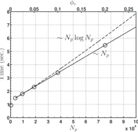
Fig. 2.ScalingoftheFCMwiththenumberofsquirmersNp.Computationaltimepertime-stepversusNp,orequivalently,versusvolumetricfractionφv.

Nc=256 coresworkinparallelforacubicdomainwith3843gridpoints.

2.3.1. Includingadditionalfeatures

WithFCM, additional effectscan readilybe incorporatedinto thesquirmer modelandinour subsequentsimulations, we considerseveralofthemtodemonstratetheversatilityofourapproach.Forexample,forcesduetostericinteractions andexternaltorquesexperiencedbymagnetotacticorgyrotacticorganismscanbeconsideredbyincludingtheminFn and

τ

_{n in Eq.(18). Additionally, we can extend the FCM squirmer model to ellipsoidal shapesby usingthe ellipsoidal FCM} Gaussian distributions.Such amodel canbe carefullytunedby comparingwithresultsfrom[55] and[56].The effectsof particle aspect ratioonsuspension properties canthen be explored systematically while still accountingforparticlesize effectssuchasJefferyorbits.Finally,wearenotlimitedtoconstantvaluesfor B1 andB2.Byallowingtheseparametersto befunctionsoftime,theFCMsquirmermodelcanbeusedtoexplorehowtheswimmers’strokesaffectoverallsuspension dynamics.TheseextensionsareaddressedinSection6.

3. Numericalmethods

3.1. Fluidsolver

The smoothness of the Gaussian force distributions allows FCM to be used with a variety of numerical methods to discretizetheStokesequations.Ithasbeenimplementedwithspectralandspectral elementmethods[42,50,49]andfinite volumemethods[57,58]inbothsimpleandcomplexdomaingeometries.

Here,weuseaFourierspectralmethodwithFastFourierTransforms(FFTs) tosolvetheStokes equations(18)–(19),for thefluidflowinathree-dimensionalperiodicdomain.WesetthezerothFouriermodeofthevelocitytozero,u

ˆ

(

k

=

0

)

=

0, toensurenomeanfluidflowthroughtheunitcell.Asthefluidencompassestheentiredomain,thisisequivalenttoadding a uniform pressuregradient to balance thenet force the particles exerton the fluid inorder to maintainthesystem in equilibrium[59,37].Thisalsoensureswe haveaconvergentevaluationofthestressletinteractions[60].As thesquirmers can movewithoutexertinga forceonthefluid, wedopermit anetmaterialfluxofsquirmers throughtheunit cell.This correspondsdirectlytothefar-fieldStokesianDynamicscomputationsperformedin[30] forsquirmersuspensions.TheFFTs are parallelized withtheMPI libraryP3DFFT.This libraryuses2D decomposition ofthe 3D domain,introducing abetter scalability than FFT libraries that implementa 1D decomposition. This decomposition hasshown good scalability up to

Nc

=

32

,

768 coresinDirectNumericalSimulation(DNS)ofturbulence[61].

3.2. Computationalwork

Asexplainedin[49],thenumberoffloating pointoperationsforFCMscaleslinearlywiththenumberofparticles,Np. WefindthesamescalingforourimplementationofFCM.Fig. 2showsthecomputationaltimepertimes-stepforNp upto 80,000particleswith3843

_∼

₆

_·

₁₀7 _{gridpointsandNc}

₌

_{256 cores.}

3.3. Stericinteractions

IncludingstericrepulsionisstraightforwardwithFCM.Theseforcesareintroducedtobothpreventparticlesfrom over-lapping during the finite time-step and to account for contact forces. For spherical particles, we use the steric barrier described in[62].Forparticlesn andm, letrnm

=

Ym

−

Yn andrnm

= k

rnm

k

.Therepulsive forceexperienced byn due to stericinteractionsis

Fb_n

₌











−

F_2aref

"

R2_ref

₋

r2_nm R2_ref

₋

4a2

#

2γ rnm, for rnm

<

Rref

,

0

,

otherwise. (29)

where F_ref is the magnitude of the force, the cut-off distance R_ref sets the distance over which the force acts, and the exponent

γ

can be adjusted to control the stiffness ofthe force. Unless specified, all the simulations are run with

F_ref

/

6

π η

aU

₌

4, R_ref

₌

2

.

2a and

γ

=

2.From Newton’s third law, we obtainFb

m

= −

Fbn.It isimportant tonote thatthis forcebarrierisgenericanditisnotintendedtomodelanyparticularphysics.Whilewecouldinsteadusean exponential DLVO-likepotential[58],theforcebarriercanbeevaluatedmorerapidlythananexponentialpotentialandbyadjustingits parameters wecan incorporaterepulsionofa similar strengthandlength scaleasDLVO forces.Athorough studyonthe effectofthisforcebarrieronthedynamicsofparticulatesuspensionsisprovidedin[62].Stericrepulsionforspheroidal par-ticlesrequiresdifferentmodeling.Inourstudy,stericforcesandtorquesare introducedbyusingasoftrepulsive potential withthesurface-to-surfacedistanceapproximatedbytheBerne–Pechukasrangeparameter[63].

Usingadirectpairwisecalculation,theevaluationofstericinteractionsbetweenallparticlepairsateachtimestepwould requireO

(

N2_p

/(

2Nc

))

computationspercore.ThiscostismuchgreaterthantheO

(

Np

)

costofthehydrodynamicaspectsof FCM.Therefore,insteadofadirectcalculation,weusethelinked-listalgorithmdescribedin[64].Thismethoddividesthe computationaldomainintosmallersub-domainsintowhichtheparticlesaresorted.Theedge-lengthofeachsub-domainis slightlylargerthan R_ref.Thesesub-domainsaredistributedoverthecoreswherethestericinteractionsareevaluated.Fora homogeneoussuspension,thisresultsinaper corecost forsteric interactionsthat is O

¡

14N2p

/(

2NcNs

)

¢

,whereNs isthe totalnumberofsub-domains.Sinceforlargesystemsizes,wehaveNs

≈

L3

/

R3_ref

≫

14 andNc

≫

1,thelinked-listalgorithm forstericinteractionsismuchmoreefficientthanthedirectcomputation.

3.4.Algorithm

Wesummarizetheoverallproceduretosimulatelargepopulationsofmicro-swimmers inStokesflowwiththeFCM:

•

InitializeparticlepositionsYn(0)andorientationsp(n0),

•

Starttimeloop:for k

₌

1

,

. . . ,

Nit

1. ComputeGaussians

1

n(k)

(

x

)

and

2

n(k)

(

x

)

,Eq.(2),

2. UpdateswimmingmultipolesG(nk),Eq.(13),andHn(k),Eq.(16),whichbothdependonpn(k), 3. Computestericinteractions,Eq.(29),withthelinked-listalgorithm,

4. Addadditionalforcingifany(gyrotactictorques,magneticdipoles,. . . ), 5. ProjecttheGaussiandistributionsontothegrid(RHSofEq.(19)),

6. SolveStokesequations,Eqs.(18)–(19),toobtainthefluidvelocityfieldu(k)

₍

_x

₎

_,

7. ComputeparticlerateofstrainsE(nk),Eq.(26), 8. If

k

En(k)

k

>

ε

,computestressletsS(nk)following[49],

a) Projectallthemultipolesontothegrid(RHSofEq.(19)),

b) SolveforStokesequations,Eqs.(18)–(19),toobtainthefluidvelocityfieldu(k)

₍

_x

₎

_,

9. ComputeparticlevelocitiesV(nk),Eq.(24),androtations

Ä

(nk),Eq.(25),

10. IntegrateEqs.(27)and(28)usingthefourth-orderAdams–BashforthschemetoobtainYn(k+1) andp(nk+1).

4. Validation

4.1. ComparisonwithBlake’ssolution

AsexplainedinSection2.3,inFCMthevelocityfieldaroundanisolatedsquirmern inaninfinite,quiescentfluidisgiven by

uFCM

₌

A

_·

Hn

+

R

:

Gn

,

(30)

whereAisasecondranktensorgivenbyEq.(21)andthethirdranktensorRcanbefoundin[38].Fig. 3shows Blake’s so-lutionEq.(12)and thevelocityfieldprovidedbyEq.(30)withtwodifferentvaluesforthedegeneratequadrupoleGaussian envelopesize,

σ

2 and

σ

2

/

2,thatappearsinthetensorA.Thestreamlinesareidentical,exceptfora near-field

recirculat-ingregion thatappears whenthewidthofthedegeneratequadrupole envelopeis

σ

2 (Fig. 3(b)).Inthisregion,however,

themagnitudeofthevelocity issmallcompared tothe swimmingspeed. Thisregion shouldnot significantlyimpact the squirmer–squirmerhydrodynamicinteractionsthatweareaimingtoresolve.

Aquantitative comparisonofthevelocityfield isprovided inFig. 4.The agreementwithBlake’ssolutionis verygood forr

/

a

>

1

.

25 when using

σ

2 forthe width ofthe degenerate quadrupole envelope.As shown inFig. 4(b),the smaller

envelopesize (

σ

2

/

2) matches Blake’ssolution moreclosely forr

/

a

<

1

.

2, withclearimprovement atthe front andrear

ofthesquirmer.Forthisenvelopesize,thevelocity fieldinducedby thedegeneratequadrupoleuFCM_B

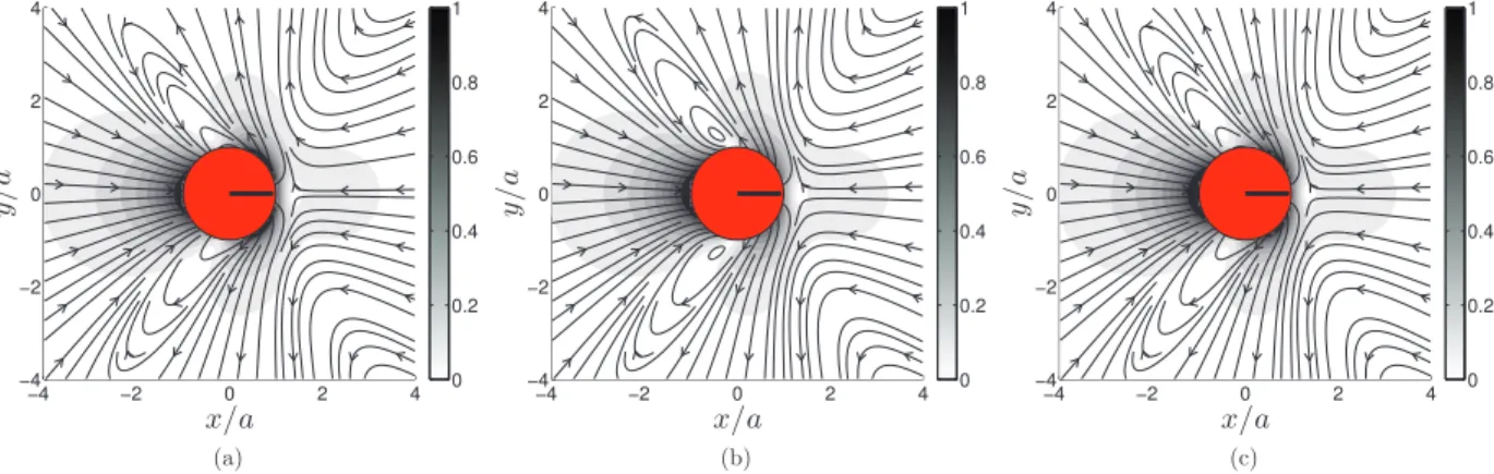
Fig. 3.Velocityfieldu/U aroundapullersquirmer(β=1)swimmingtotheright.(a)Blake’ssolution;(b)FCMsolutionwith σ2 forthedegenerate

quadrupoleenvelope.(c)FCMsolutionwithσ2/2 forthedegeneratequadrupoleenvelope.

Fig. 4.ComparisonwithBlake’ssolution,Eq.(12).(a)Normalizeddifference,kuBlake_−uFCM_{k/U ,betweenFCMandBlake’ssolutionforapullersquirmer} (β=1).Thehalf-widthforthedegeneratequadrupoleenvelopeisσ2. :10% iso-value.(b)VelocityprofilealongtheswimmeraxisforBlake’s

solutionandtheFCMapproximationforthetwodifferentdegeneratequadrupoleenvelopesizes.

analytical solution uB1 in Eq.(12) (not shownhere). Below this width no quantitative improvement is observed as the remainingerrorcomesfromthedipolarcontribution,uB2.

Whilethisquantitativecomparisonprovidesanicewaytochoosethedegeneratequadrupoleenvelopesize,wemustalso keep inmindthecomputational costassociatedwithdecreasingthislengthscale.Eventhough itwouldyieldaflowfield slightlymoreinregisterwithBlake’ssolution,resolvingthelengthscale

σ

2

/

2 ina3Dsimulationwouldrequireagridwith

8timesasmanypoints asthatneededfor

σ

2,thesmallestlength-scalealreadyinFCM.Thiswouldincreasecomputation

timesby atleastan orderofmagnitude. Inaddition,theFCM volume averagingusedto determinethesquirmer transla-tional andangularvelocities,Eqs. (3)–(5),will reduce thecontributionof thelocalizedvelocity field discrepancies tothe squirmer–squirmerinteractions.Inoursubsequentsimulations,wethereforeutilize

σ

2 forthedegeneratequadrupole

en-velopesizesincereducingthislength-scalewouldsignificantlyincreasethecomputationalcost,butonlyprovideaminimal improvement.

4.2. Pairwiseinteractionsofsquirmers

In[28],theauthorsperformeda varietyofsimulationsusingtheBoundaryElementMethod(BEM)tocomputetohigh accuracythepairwiseinteractionsbetweenasquirmerandaninertsphere,andbetweentwosquirmers.Here,weconsider thesamescenariosasthoseauthorsandcompareresultsfromourFCMsimulationswiththeirBEMresults.

4.2.1. Interactionsbetweenasquirmerandaninertsphere

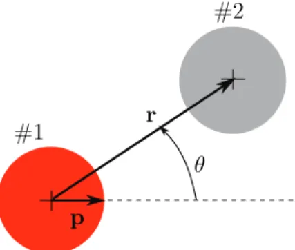
Wefirstconsidertheinteractionsbetweenaninertsphere(labeled “2”)locatedatapointrfromthecenterofapuller squirmer(labeled “1”)with

β

=

5.Thedirectionr

/

r formstheangle

θ

withtheswimmingdirectionpofthesquirmer.The problemsetupisdepictedinFig. 5.

Fig. 5.Sketch showing the set-up of our computations of the interactions between squirmer “1” and inert sphere “2”.

Fig. 6.The(a)radialvelocity|Ur,2|,(b)angularvelocity|Äz,2|,(c)stressletcomponent|Sxx,2|,and(d)stressletcomponent|Sxy,2|fortheinertsphere“2” atadistancer fromapullersquirmer(β=5).

Fig. 6comparesthevelocityofthesphereobtainedusingFCMsimulationswiththeBEMresultsandfar-fieldanalytical solutionsfrom[28].Wecomputedthefar-fieldvelocityinFig. 6(a)usingtheexpressionsprovidedin[28] sinceitwasnot plottedin Fig. 6(a) of [28] forr

/

a

<

2

.

5. We suspect that the BEM resultswere also not plottedfor thisrange.As FCM alsoresolves themutuallyinduced particlestresslets,itprovides amoreaccurate estimationthan far-fieldapproximation of[28].Asaresult, weseethattheFCM resultsverycloselymatchBEM,evenintherangewherer

/

a

<

3.Similartrends areobserved forthe angularvelocity oftheinertsphere (Fig. 6(b)) andthestressletcomponents (Figs. 6(c), 6(d)).These comparisonsillustratetheaccuracyoftheresultsthatcanbeobtainedusingFCM,whichcloselymatchesBEMbutincursa fractionofthecomputationalcost.

Fig. 7.Initial configuration of the squirmers in the trajectory simulations.

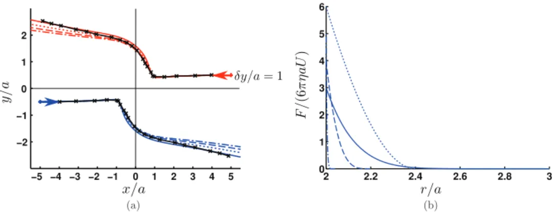
Fig. 8.Trajectoriesoftwosquirmersswimminginoppositedirectionswithtransverseinitialdistanceδy=1a,. . . ,10a.Lines:datafrom[28].Symbols:FCM results.

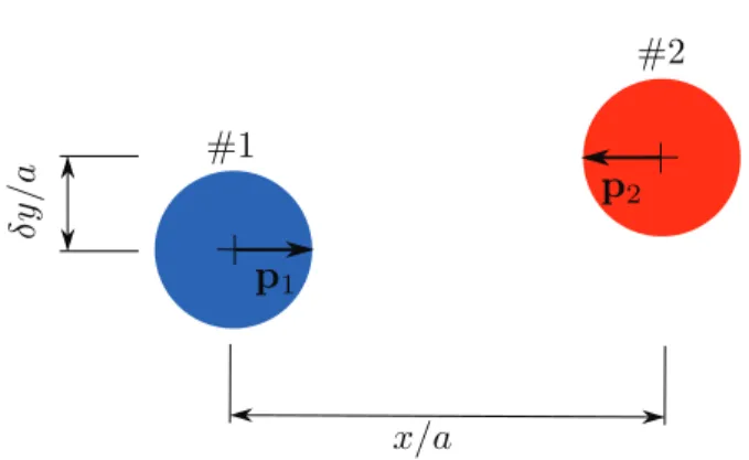
4.2.2. Trajectoriesoftwointeractingsquirmers

Wecomputethetrajectoriesoftwopullersquirmers(

β

₌

5)andcomparetheresultswiththeBEMsimulationsof[28]. One squirmerinitially swimsin thex-direction, p1

=

ex,andtheother one intheopposite direction, p2

= −

ex. Theyare placed with initial separation distance

δ

y

₌

1a

,

. . . ,

10a inthe transverse direction and

δ

x

₌

10a in the x-direction. The problemset-up isdepictedinFig. 7.Since thesquirmers maycollide,we alsoincludesteric interactionsprovided bythe forcebarrier(29).

As shownin Fig. 8, the trajectories match very well with the BEM results for

δ

y

_≥

2a. When

δ

y

₌

1a, the collision barrier andnear-field hydrodynamic interactions play an importantrole in determiningthe overall squirmer trajectories.

Fig. 9showstheeffectofthestericrepulsionparameters F_ref andR_ref on thesquirmertrajectories.The specificvaluesof theseparameters are provided inAppendix B.We seethat by varying thebarrier parameters onecan obtain trajectories thatcloselymatchtheresultsof[28].

5. Simulationresults

5.1. Largesuspensionsofswimmingmicro-organisms

The squirmer model has been widely used to investigate both the behavior of singleswimmers [65–68], aswell as their collectivedynamicsandinteractions [29,30,69,34,33].Simulationsofsuspensionsrevealedthattheoverallpopulation dynamicsdependstronglyonthesquirmingparameter

β

.Inparticular,when

|β|

issmall,theisotropicstateforaperiodic suspensionhasbeenshowntobeunstable,andthesuspensionevolvestoapolarsteady-statewithanon-zerovalueofthe polarorderparameter

P

(

t

)

₌

¯

¯

¯

¯

¯

¯

1 Np Np

X

n=1 pn

(

t

)

¯

¯

¯

¯

¯

¯

.

(31)

Fig. 9.Influenceofthecollisionbarrierparametersonthesquirmertrajectoriesforthecasewhereinitiallyδy=1a.(a)Trajectories.Crosses:datafrom

[28].(b)Forcebarrierprofiles(seealsoAppendix B).Thelinestylescorrespondthoseshowingthetrajectoriesin(a). :barrierusedinFig. 8.

Fig. 10.Snapshotsoftheorientationalstateinasemi-dilutesuspension(φv=0.1)containingNp=37,659 swimmerswithβ=1.hpiisthemean

steady-stateorientationvectorontheunitspheredefinedinEq.(32).pn· hpiquantifiesthedegreeofalignmentwiththemeandirectionhpiofswimmer n.

Thisinstabilityhasbeenstudiednumericallyby[30] and[69] usingStokesian dynamicswithNp

=

64 swimmersfor vol-umefractions

φ

v

=

0

.

01

→

0

.

5.UsingtheLattice-Boltzmannmethod,[34]observedthesamebehavior for Np

=

2000 and

φ

v

=

0

.

1.

5.1.1. Polarorderparameter

Using ourFCM model, we studythisinstability andthe resulting polarorderof a squirmersuspension. In particular, we examinehowthe domainsize affectsboth thegrowthrateofthe instabilityandthe finalsteady-state.The influence ofdomain size hasnot been addressedpreviously for squirmer suspensionsthough it hasbeen observed insimulations ofrod-likeswimmers [25]. We performsimulations of semi-dilutesuspensions (

φ

v

=

0

.

1) of pullersquirmers (

β

=

1) in triply-periodicsquaredomains withedgelengthsrangingfromL

/

a

₌

14 to L

/

a

₌

116.Asthevolume fraction

φ

v isfixed, varying L

/

a increasesofthenumberofswimmersfrom Np

=

64 (asin[30,69]) to Np

=

37

,

659.Weinitializea homoge-neous,isotropicsuspensionby distributingtheswimmer positionsuniformlyinthedomainandtheswimmingdirections uniformlyovertheunitsphere.Dependingondomainsize,thesimulationsareruntofinaltimetf

=

1000

−

1500a

/

U with atimestep

1

t

₌

0

.

005a

/

U .Thus,eachsimulationrequiresbetween2

×

105–3

×

105time-steps.

Fig. 10illustrates the polar ordered state for a simulations with L

/

a

₌

116, Np

=

37

,

659. We quantifythe degree of alignmentofeachswimmern,pn

· h

p

i

,withthemeansteady-stateorientation

h

p

i

givenby

h

p

_{i =}

lim t→∞ 1 Np Np

X

n=1 pn

(

t

)

P

(

t

)

,

(32)

where

h

p

_i

lies on the unit sphere

S

2_.At t

₌

0, there is no clear mean orientation, while at t

₌

1000a

/

U ,a significant proportionofparticlesarealignedwiththemeandirection

h

p

_i

.

Fig. 11.PolarorderP(t)inasemi-dilutesuspension(φv=0.1)ofsquirmerpullers(β=1).(a)Timeevolutionofpolarorderdependingonthenumberof

swimmers. :L/a=14,Np=64; :L/a=19, Np=174; :L/a=38,Np=1395; :L/a=58,Np=4707; :L/a=77,

Np=11,158; :L/a=116,Np=37,659.(b)SteadystatevalueP∞dependingonNp∼ (L/a)3. :fitlinearwith1/pNp.(Inset):Dependence

ofP∞_with1/pNp.

Fig. 12.Characterizationofthepolarinstability.(Mainfigure):Timeevolutionofpolarorderinsemilogarithmicscalesuggestsanexponentialgrowthof theinstability.(Inset):GrowthrateoftheinstabilityfordifferentNp(andL/a).

Fig. 11ashows P

(

t

)

,Eq.(31),for thesimulations with differentdomain sizes.For each domainsize, we see that the suspension evolvesfromtheinitial isotropicstate to onethat haspolarorder. Weobserve,however,that the finalvalue,

P∞_{,ofthepolarorderparameter dependsonthedomain size.We findthatit decreases asL}

_/

_{a (and Np) increases.The}

dataalsoshowsthatasL

/

a

_{→ ∞}

, P∞ _decayslike

₍

_L

_/

_a

₎

−3/2 _{(or N}−1/2

p )andreachesanasymptoticvalueof P∞

→

0

.

452. Theseresultswouldindicate thatpolarordershould alsoariseinan unbounded suspension.Wealso observethatinthe polarorderedstate, theaverageswimmingspeed is4%less thanitsvalue inisotropicstatewhichitselfisnearly thefree swimmingvalue.Indeed,weremindthatinoursimulations,azeronetfluxofthesuspensionisimposed,therefore,when theswimmersarealigned,theyaresloweddownbythebackflow.

Fromoursimulations,wemayalsoanalyze howL

/

a affectsthetimeevolutionoftheinstability.InFig. 11(a),weclearly seethatthetimeittakestoreachthefinalpolarstate increaseswithdomainsize.Weanalyzethisdatainmoredetailin

Fig. 12,nowplottingitin semilogarithmicscale. Foreach case,we findthat afteraninitial transientstate, theinstability growsexponentiallyandwithagrowthratethatisindependentofthesystemsize(seeinsetfigure).Itwouldcertainlybe interestingtoinvestigateifthisresultcouldbereproducedbyalinearstabilityanalysisofcontinuummodelforasquirmer suspension.

5.1.2. Orientationaldistribution

Wecan examinethepolarorderinmoredetailbycomputingtheorientationaldistribution

9(θ,

φ,

t

)

definedoverthe unitsphere[70].Here,

θ

₌

cos−1

(

pz

)

correspondstotheelevationanglewhile

φ

=

tan−1

(

py

/

px

)

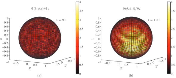
givestheazimuthalangle.

Fig. 13.Orientationaldistributionontheunitsphere(φ,θ ).(a)Distributionbeforethetransitiontopolarorder:tU/a=90.(b)Distributiononcethepolar orderedstateisreached:tU/a=1110.

Fig. 14.Time-averagedsteady-stateorientationaldistributionintheframeofthemeanorientationvector9(θ,φ)|hpi.(a)Distributionovertheunitsphere.

(b) :distributionofelevationangleθaveragedoverazimuthalangleφ; :uniformdistribution90(θ )=1/π; :distributionof az-imuthal angleφaveragedoverelevationangleθ; :uniformdistribution90(φ)=1/(2π).

Fig. 13shows

9(θ,

φ,

t

)

normalizedby theisotropicdistribution

9

0

=

1

/(

4

π

)

attimesbeforeandafter thetransitionto polarorder for the case where Np

=

11

,

158 and L

=

78a. As expected, before the transition, the distribution is nearly uniformoverthesurfaceofthesphere.Afterthepolarstateisreached,weseethat

9(θ,

φ)

isnarrowlydistributedaround the mean direction

h

p

_i

. We note that the steady state mean direction depends both on the random initial seeding of swimmers and the domain geometry. We find that system first aligns along an arbitrary direction due to the random initialseedingofswimmers,butastimegoeson,themeandirectortendstoalignwiththenormaltooneoftheperiodic boundaries.Asaconsequence,thesteadystatemeandirectionisbiased bythedomainshapethatbreaksradialsymmetry. We would like to stress that, however, asdemonstrated here andin [30], the polarordering itself is a consequence of squirmer hydrodynamic and steric interactions rather than the domain shape. Fig. 14 shows the steady-state averaged distribution

9(θ,

φ)

|

hpi in the frame where the mean direction isgiven by

θ

=

0 and

φ

=

0. We see that the resulting

distributionisaxisymmetricinthatitdoesnotdependon

φ

.Thisisnotsurprisingastheflowfieldinducedbyasquirmer isaxisymmetric.Orientationaldistributionscouldalsobe obtainedfromcontinuummodels,aswasdoneforswimmersin externalflow fields[70]. Ourresultscouldbe comparedwithcontinuum models ofsquirmersuspensions,though,to the bestofourknowledge,thecontinuum modelsthat arecurrentlyavailable intheliterature predictastableisotropicstate forsphericalswimmersuspensions.

5.1.3. Spatialdistribution

Alongwiththeorientationaldistribution,wealsoexaminethespatialdistributionofsquirmersbycomputingtheVoronoi tessellation forthe set of points corresponding to the squirmers’ centers. We have used the C++ libraryVoro++ [71] to

Fig. 15.DistributionofVoronoicellvolumes.(Mainfigure):Timedependenceofthestandarddeviation,σV,oftheVoronoivolumedistributionnormalized

bythemeanvaluehVVi.(Inset):TimeaverageoftheVoronoivolumedistributionbefore( )andafter( )thepolarordertransition.

Fig. 16.Steady state pair distribution function (a) g(r, θ ). (b) g(r).

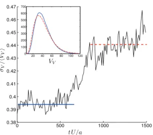
performthecomputationanddeterminethevolume, VV,ofeachVoronoicell.Fig. 15showstheevolutionofthestandard deviation,

σV

, of the VV distribution for the case where Np

=

11

,

158 and L

=

78a. We see sudden increase in

σV

as the suspensiontransitions topolarorder,corresponding toa wideningofthedistribution.The insetinFig. 15 showsthe time-averaged distribution before and after the transition. Before polarordering occurs, the mode ofthe distribution is

¯

VV

≈

34a3,which is slightlyless than theaverage value

h

VV

i

=

L3

/

Np

=

42a3 that one might expect.During the polar steady-state,wefindthatthemodedecreasesto V

¯

V

≈

30a3,whichisindicativeofaslightclusteringoftheparticles.

Tofurtherexaminethespatialdistribution,wecomputethesteady-statepairdistributionfunctiong

(

r

,

θ )

whichgivesthe probabilityoffindingasquirmeratadistancer

_{= |}

r

_|

andwithelevationangle

θ

=

cos−1

(

r

_·

p

/

r

)

fromanothersquirmerthat hasswimmingdirectionp.Fig. 16(a)showsg

(

r

,

θ )

forthecasewhereNp

=

11

,

158 andL

=

78a.Weseeclearlythatg

(

r

,

θ )

dependsnotonlyonr,buton

θ

aswell. Atsteady-state,foragivensquirmerthereisasignificantly higherprobability of finding anothersquirmer infront ofit (

θ

=

0) ratherthan behind it.If we integrate g

(

r

,

θ )

over

θ

,we obtain theradial distribution functionshownin Fig. 16(b).Wefind that g

(

r

)

exhibitsa peakattwo radii fromtheswimmer surface. This peaksuggeststheexistenceofparticleclusterswhosesizesaregreaterthantwoindividuals.

5.1.4. Orientationalcorrelations

The hydrodynamic and steric interactions between the squirmers also lead to correlations in their orientations. We computethesteady-stateorientationalcorrelationfunction[30]

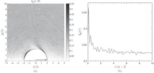
Fig. 17.Correlations in squirmer orientation at steady state. (a) Ip(r, θ ). (b) Ip(r).

where the brackets

h·i

denote the ensemble average that we compute by averaging over both time andsquirmer pairs.

Fig. 17(a)showsthecorrelationsinthe frameofasquirmer locatedattheoriginandwithp

_{= ˆ}

z andthe definitionsofr

and

θ

areidenticaltothoseinSection 5.1.3.Wefindthat thehighestcorrelationsoccurnearcontact(r

≈

2)attheangles

θ

≈

π

/

3 and

θ

≈

3

π

/

4.Despitetheoverallpolarorder,wecanidentifytwodistinctregionsaround

θ

=

0 and

θ

=

π

where theorientationsareuncorrelated.Wedo,however,findapositivevalueforthecorrelations,evenfarawayfromtheorigin. Thisismostevidentinthe

θ

-averagedcorrelation, Ip

(

r

)

,showninFig. 17(b)whichapproachesafinitevalue Ip

=

0

.

22 as

r increases.Thisisconsistent withtheobservedlong-rangepolarorderofthesuspension.We alsofindthat Ip

(

r

) >

0 for all r.Thisagainmaybearesultofthestrongpolarorderingofthesuspension.

6. Extensionstoellipsoidalswimmersandtime-dependentswimminggaits

Inthissection,wedemonstratetheextensionofourapproachtobothspheroidalswimmershapesandtime-dependent swimming gaits. This illustrates the versatility of FCM while preserving good computational scalability and an accurate treatmentofhydrodynamicinteractions.

6.1. FCMforellipsoidalparticles

ToextendFCMtopassiveellipsoidalparticles,onesimplymodifiestheGaussianenvelopesinEq.(2) [50].Forexample, takingthe orthonormal vectors e

ˆ

1, e

ˆ

2, and e

ˆ

3 to be aligned withthe ellipsoid semi-axes having lengths a1, a2, and a3 respectively,theGaussianenvelopecorrespondingto

1

n

(

x

)

is

1

ell_n

(

x

)

_{= (}

2

π

)

−3/2

(

σ

1;1

σ

1;2

σ

1;3

)

−1exp

·

−

1₂

(

x

₋

Yn

)

T

Q

T

6

1

Q

(

x

−

Yn

)

¸

(34)

where

σ

1;i

=

ai

/

√

π

fori

=

1

,

2

,

3,

Q

= (ˆ

e1 e

ˆ

2 e

ˆ

3

)

,and

6

₁

₌







σ

₁−_;2₁ 0 0 0

σ

₁−_;2₂ 0 0 0

σ

₁−_;2₃





 .

(35)

Asimilarexpression isusedfor

2

elln

(

x

)

with

σ

2;i

=

ai

/

¡

6

√

π

¢

1/3.Beyondthis,theunderlying algorithmofprojectingthe particleforcesontothefluidandvolumeaveraging theresultingfluidflowremains unchanged.Theconstraintthat En

=

0 foreach n isstill usedto find thestresslets. Thus, usingFCM to compute the motionand hydrodynamic interactions of ellipsoidsdoesnotrequireanyadditionalsteps inthealgorithmdescribed inSection 3.4.AsexplainedinSection 3.3,the modeling ofstericinteractionsdiffers fromthat forsphericalparticles andoursimpleforce barriercouldnotbe used.An extensivevalidationofFCMforellipsoidalparticlesispresentedin[50] wheremanyoftheclassical resultsforellipsoidal particles inStokes flow, e.g. Jeffery’s orbits,are shownto be recovered exactlywith FCM.We note that for veryslender particles,FCMwouldnotbeappropriateandcomputationsbasedonslender-bodytheories[72]shouldbeperformed.

Fig. 18.Simulationofadilutesuspensions, φv=0.05,ofprolate spheroidalpushers,B2= −1.5, B1=0,withaspectratio aa12 =

a1

a3 =3.(a)Snapshot

att=30U/a1.Colorsindicatethevelocitymagnitudenormalizedbytheindividualswimmingspeed.(b)TimeevolutionofpolarorderP(t). : isotropicvalueofthepolarorderparameter1/pNp=0.026.

To extend FCM to active ellipsoidalparticles requires addingthe stresslet and possible potential dipole termsto the multipoleexpansion.Asforsphericalparticles(seeSection2.3,Eqs.(20)and(23)),theseadditionalmultipoleswillleadto artificial, self-inducedvelocitiesandlocalrates-of-strain.Theseeffectsmustbesubtractedaway usingtheformuladerived inAppendix A.ItisworthreiteratingthatthesearetheonlystepsthatneedtobeaddedtotheFCMalgorithmforpassive particlestosimulateactiveones.

6.2. Spheroidalswimmersimulations

Previousparticle-basedsimulations[25,32]andcontinuumtheoryresults[18–20]predictanunstableisotropicstatefor suspensionsofprolatespheroidalpushers.UsingFCM,wesimulateadilutesuspension,

φ

v

=

0

.

05,ofNp

=

1500 spheroidal pushers with aspect ratio a1

a2

=

a1

a3

=

3. For these simulations, the stressletparameter is B2

= −

1

.

5 and the degenerate quadrupole isset tozero, B1

=

0. Stericinteractions are includedby usinga softrepulsive potential witha

∼

r−5 decay andsurface-to-surfacedistanceapproximatedbytheBerne–Pechukasrangeparameter[63].Fig. 18(a)showsasnapshot of thesuspension whereclustersofswimmershavevelocities nearly1

.

6 timeslargerthan theisolatedswimmingspeed.As in[25,32],weseethattheisotropicstateisnot stableandthepolarorderparameterincreaseswithtime(Fig. 18(b)).We donotseeaslargean increasein P

(

t

)

asin[25,32]duetotherelativelylowaspectratioofourswimmers.Thetumbling effectduetoJefferyorbitsandthesterictorquesthat tendtoalignadjacentswimmersaremuchlower thanthey arefor rod-likeswimmers.

6.3. Suspensiondynamicsoftime-dependentswimmers

Here,weshowhowtoincorporatetime-dependenceintoourmodel.Usingtheprocedureoutlinedin[73],wedetermine thetime-dependentmultipolecoefficients B₁

(

t

)

andB₂

(

t

)

fromtheexperimental dataprovidedin[39].Wethenperform suspension simulations thatshow time-dependenceatthelevel ofindividualswimmerscan affecttheoverall suspension properties.

6.3.1. Asingletime-dependentswimmer

Recentexperiments[39]quantifiedtheperiodicswimminggaitandresultingflowfieldofthealgaecellChlamydomonas Rheinardtii.Theyextractedtheswimmingspeed,theinducedvelocityfield,andthepowerdissipation,showingalsothatall canberepresentedasperiodicfunctionsoftime.Arecenttheoreticalinvestigation[73]showedthatthesequantitiescould bereproducedusingamultipole-basedmodel.Intheirstudy,theyconsideredthreetime-dependentmultipoles:a stresslet, adegeneratequadrupole(orpotentialdipole)anda“septlet”.Thestressletdecaysasr−2_{whereasthedegeneratequadrupole} andthe“septlet”decayliker−3_{.Here,weutilizeonlythestressletanddegeneratequadrupoletermsandfindthattheyare} sufficienttoreproducethefeaturesmeasuredby[39].

Themeasuredswimmingspeedfrom[39],U

(

t

)

,canberepresentedusingthetruncatedFourierseriesintime(see[73]):

U

(

t

)

₌

a0

+

a1cos

(

ω

t

)

+

a2cos

(

2

ω

t

)

+

b1sin

(

ω

t

)

+

b2sin

(

2

ω

t

)

(36)

where

ω

is the frequencyof the swimming gait. The mean swimmingspeed over one beatperiod, T

₌

2

π

/

ω

, is given by a0

=

49

.

54a s−1,where a

=

2

.

5 µm is the radius ofthe microorganism. The values forthe remaining coefficientsare

Fig. 19.(a) (B1(t), B2(t)) phase diagram for one beat cycle. (b) Power dissipation5d(t)over one beat cycle. : FCM, : results from[39].

providedinthe supplementaryinformationof[73].From Eq.(9),we canimmediatelydetermine thetime-dependent de-generatequadrupolestrength

B1

(

t

)

=

3

2U

(

t

)

(37)

inordertopreserve theinstantaneousforce-freecondition. Unlikethisterm, thereismorethan oneway tocalibrate the stressletstrength,B2

(

t

)

.Forexample,onecoulddetermineB2

(

t

)

usingthepowerdissipationmeasurementsfrom[39] and Eq.(9)from[74]

5

d

(

t

)

=

2 3

π η

a

³

8B1

(

t

)

2

+

4B2

(

t

)

2

´

(38)

forthe power dissipated by a squirmer. Using this approach,we found that ourresulting flow field did not match the experimental results from [39]. We instead determine B2

(

t

)

directly from the experimental flow field by fitting to the location of the moving stagnation point. Thisis the same approach adopted by [73]. We utilize three Fouriermodes to describethetimeevolutionof B₂

B2

(

t

)

=

c0

+

c1cos

(

ω

t

+

ϕ

c1

)

+

c2cos

(

2

ω

t

+

ϕ

c2

)

+

c3cos

(

3

ω

t

+

ϕ

c3

)

+

s1sin

(

ω

t

+

ϕ

s1

)

+

s2sin

(

2

ω

t

+

ϕ

s2

)

+

s3sin

(

3

ω

t

+

ϕ

s3

) ,

(39) wherethe amplitudes c0

,

c1

,

s1

,

. . .

andphases

ϕc1

,

ϕs1

,

. . .

are fittedmanually. Appendix C givesthe resulting valuesof theseparameters.

ThephasediagraminFig. 19(a)showsthevalueof B₁ versus B₂ anditissimilartothatfoundby[73].Weextractthe averagevalueof

β(

t

)

=

B₂

(

t

)/

B₁

(

t

)

overonebeatcycle

¯

β

₌

1 T T

Z

0 B2

(

t

)/

B1

(

t

)

dt

=

0

.

1 (40)

whichcorresponds to apullersquirmer witharelatively smallstressletmagnitude. Fig. 19(b)showsthe resultingpower dissipationasdetermined fromEq.(38).Itreachesapeakvalueatt

/

T

_≈

0

.

3,whichcoincideswiththetime atwhichthe swimmingspeed reachesits maximumvalue. We note that unlike [39] ourswimmers generateaxisymmetric flowfields andweareconsideringa3Dperiodicdomain.Despitethis,weachieveaqualitativelysimilarpowerdissipationprofilewith slightlygreatervaluesduringthefirsthalfofthebeatcycle.

Fig. 20showstheflow fieldaround ourmodelofC.Rheinardtii atsixdifferenttimesduringits beatcycle.Thesetime points arechosen to correspond tothose inFig.3 of[39]. Weachieve very similar streamlinesand, by construction,the positionof thestagnation point matches theexperimental data very well. We alsonote that our flow field is similar to thatgivenbythemultipolemodelfoundin[73]eventhoughwedonotincludetherapidlydecaying“septlet”terminour model.Theseresultsillustratethatourproperlytuned,time-dependentsquirmermodelcanyieldflowfieldsverysimilarto thoseofrealorganisms.

Fig. 20.Snapshotsofthetime-dependentflowfieldaroundamodelChlamydomonas.Backgroundgreylevelsrepresentthenaturallogarithmofthenorm ofthevelocityfieldinrad s−1_{. :positionofthestagnationpointgivenbytheFCMmodel. :positionofthestagnationpointmeasuredby[39].(Insets)} Swimmingspeedalongthebeatcycle.

Fig. 21.RelativetrajectoriesoftwomodelC.Rheinardtii swimminginoppositedirectionswithstrokephaseshift1ϕandinitialtransversedistanceδy=1a and2a.Thegreylevelslightenas1ϕincreasesfrom1ϕ=0→ 1ϕ=7π/4. :trajectoryoftwosteadysquirmerswithβ=0. :trajectoryof twosteadysquirmerswithβ=0.1.(Top)δy=1a.(Bottom)δy=2a.

6.3.2. InteractionsbetweentwomodelC.Rheinardtii

We first consider pairwise interactions betweentwo model C.Rheinardtii for two initial configurations,

δ

y

₌

1a and 2a (cf. Section 4.2.2). We introduce a phase shift,

1

ϕ

, between their swimming cycles. When

1

ϕ

=

0, the swimmers are synchronized,whereas for

1

ϕ

₌

π

they are completelyout of phase.Fig. 21 showsthe effectofthisphase shifton the trajectories. For each case, we show only the trajectory of the swimmer labeled “2” in Fig. 7. We also provide the trajectories ofsteady swimmerswith

β

=

0 and

β

=

0

.

1 for comparison. Recall that

β

=

0

.

1 corresponds to the average value of B2

(

t

)/

B1

(

t

)

in ourmodel.Wesee thatthe trajectories,includingthefinal positionsandorientations,dodepend

Fig. 22.Sketchofthesimulationswithtime-dependentswimmers.Eachswimmern generatestime-dependentflowdisturbanceswiththesameamplitude andfrequency,butthephase1ϕnmaybedifferentforeachswimmer.

on

1

ϕ

.Wefind,however,thatthesevariations aresmallcomparedto theswimmerseparation distance(see theinsetof

Fig. 21fortherelativetrajectoriesintheframeofoneswimmer).Thetrajectoriesarealsoclosetothoseforsteadysquirmers with

β

=

0

,

0

.

1.

6.3.3. Collectivedynamicsoftime-dependentswimmers

Inthissection,wepresentresultsfromsuspensionsimulations usingourunsteadymodelforC.Rheinardtii. Tothebest of our knowledge, similar results have not appeared in the literature. We aim to show in this initial study that time-dependenceofindividualswimmerscanaffecttheir overalldistribution.Specifically,weshow thatthedistributionofbeat phasesaffectsthesteady-statepolarorderofthesuspension.Fig. 22showsasketchofthesimulationswithtime-dependent swimmers.

Weconsider asuspension of Np

=

1395 time-dependentswimmers distributeduniformlyina triply periodicdomain. Thevolumefractionis

φ

v

=

0

.

1.Wetake theinitialswimmingdirectionstobedistributeduniformlyovertheunit-sphere. Forswimmern, itsgaitis characterizedby B₁

(

t

_{+ 1}

ϕn

)

and B₂

(

t

_{+ 1}

ϕn

)

, where

1

ϕn

isthe valueof itsbeatphase. We considertwodifferentdistributionsofthebeatphases.Thephasesareeitheruniformlydistributedwith

1

ϕn

_{∈ [}

0

;

2

π

_]

,or

1

ϕn

=

0 for all n such that all swimmers are synchronized.We run the simulations for3700 dimensionlesstime units, corresponding to 4000beat cycles.As mentioned in Section 6.3.1, the meanvelocity of C.Rheinardtii is U

₌

49

.

54a s−1_. Sincewetakethetime-step

1

t

₌

0

.

0025a

/

U ,thetotaltimeforoursimulationscorrespondto1

.

5

×

106

1

t.

Fig. 23(a)showstheevolutionofthepolarorderparameterforthesetwodistributionsofbeatphase.Alsoshownisthe polarorderparameterforsuspensionsofsteadyswimmerswithswimmingspeedsequaltothemeanswimmingspeedfor thetime-dependentcaseandeither

β

₌

0 or

β

₌

0

.

1.Wefindthatwhenthereisauniformdistributionofthebeatphase, weachieveresultsthatmatchthesteadycasewith

β

=

0

.

1.Ontheotherhand,iftheswimmersaresynchronized,wefind thatthepolarorderparametermatchesthatforthesteadycasewith

β

=

0.Fig. 23(b)showsthesteady-stateorientational distributions

9(θ )

_|

_hpiaboutthemeandirector.Again,weseethatthedistributionforcaseofauniformdistributionofbeat

phasesmatchesthatforthesteadycasewith

β

=

0

.

1,whilethesynchronizedsuspensionhasthesamedistributionasthe

β

=

0 case.Thesenewresultsshow that thedistributionofbeatphasescanstronglyaffecttheorientational orderofthe suspension.

Fig. 23.Polarorderparameterandorientationaldistributionforsuspensionsofsteadyandtime-dependentswimmers. :time-dependentswimmers withrandom phase; :synchronizedtime-dependentswimmers; :steady swimmerswithβ₌0; :steady swimmerswith β₌0.1. (a) Timeevolutionofpolarorder.(b)Steadystateorientationdistributionaroundthemeandirector9(θ )|hpi. :uniformdistribution90(θ )=1/π.

7. Conclusions

In thisstudy, we presentedan extension of FCM to compute the hydrodynamic interactions betweena large number (104_–105_{) of active self-propelled particles insemi-dilute suspensions.Our approach buildsfrom the sphericalsquirmer} modeldevelopedbyBlake[27]byincludingintheusualFCMforcedistributiontheregularizedsingularitiesthatcorrespond to the surface squirming modes. We haveshownthat our modelreadily allows fordifferent swimminggaits,as well as spheroidal swimmer shapes, andcan alsoaccount foreffects such assteric repulsion. Wedemonstrated the accuracy of our model by comparing velocity fields, pairwise interactions, and trajectories with the analytical or numerical results given by the full squirmer model.In oursquirmer suspension simulations, we recovered the polar orderfound in other studies, butalso quantified the effects of domain size on the final steady-state. Specifically, we showed that for puller suspensionswith

β

₌

1,thefinal valueofthepolarorderparameterdecreasesandthetime neededtoreachsteadystate increasesasthesystemgetslarger.Wedid,however,findthatthesequantitiesappearedtoconvergetoanasymptoticvalue and that polar order should be present even for an infinitely large domain. The scale of our simulations allowed usto compile robust statisticsandexamine indetailthe orientationaldistribution andlocalmicro-structureof thesuspension. Byextendingthemodeltotime-dependentswimminggaits,wealsoillustratedforthefirsttime,tobestofourknowledge, thattime-dependenceatthelevelofindividualswimmerscanaffectthefinalsteady-statedistributionofthesuspension.

We see that the squirmer model within the FCM framework provides an effective computational approach to simu-late active suspensions, allowing for particlenumbers that begintoapproach continuum levels. As aresult, we feel that our computationalmodel canboth be usedto complementexperimental research,aswell asinform the development of continuum models.Forexample,wehaveshownthatthetime-dependency ofswimminggaitscanbereadilyincludedin our modelby tuning it toavailable experimental data [39]. Bytuning our modelto similar experimental data,butfora wider zoologyof microorganisms[9],we could assessthe possibledifferencesin collectivedynamicsexhibited by differ-ent species,orevenlookinto howone speciesmightinteractwithanother.In addition,ourmodelcould be an effective approachtoaddressquestionsregardingthemixingofbackgroundscalarfields[33] orpassivetracersdynamics[75,76]in active,time-dependentsuspensions.TheeffectsoftracerBrownianmotion[47] canbeincludedwithsquirmermodeland thecompetitionbetweentracerdiffusionandadvectionduetotheflowsproducedbytheswimmerscanbeassessed.

Acknowledgements

The authorswouldlike tothankProf. MartinMaxey formanyinsightfulcomments andacknowledge hisinstrumental role inbringing theauthorstogethertocarry outthiswork.WewouldalsoliketoacknowledgeProf.RaymondGoldstein, Dr.Ottavio Croze,NavishWadhwa andProf.PierreDegond forinteresting discussions.We arealsogratefulto Annaig Pe-dronoandDr.PascalFedeforprovidinghelpful supportonnumericalissues.Thisworkis developedwithinthe MOTIMO ANRProject.SimulationswereperformedontheCalmipsupercomputingmesocenter.WethankINPTforfundingthe inter-nationalcollaborationbetweenIMFTandImperial College(grantno.SMI2014).Wewouldalsoliketoacknowledgetravel supportfromEPSRCMathematicsPlatformgrantEP/I019111/1.

Appendix A. Self-inducedeffectsforspheroidalswimmers

Inthisappendix,weshowhowtocomputetheartificialself-inducedeffectsduetothesquirmingmodes(seeSection2.3) forthecaseofspheroidalswimmersdescribedinSection6.1.