QMOM-based population balance model involving a fractal dimension for the flocculation of latex particles

O

pen

A

rchive

T

oulouse

A

rchive

O

uverte

(OATAO)

OATAO is an open access repository that collects the work of some Toulouse

researchers and makes it freely available over the web where possible.

This is an author’s version published in:

http://oatao.univ-toulouse.fr/

20497

Official URL:

https://doi.org/10.1016/j.ces.2016.07.044

To cite this version:

Vlieghe, Mélody and Coufort, Carole and Liné, Alain and Frances, Christine

QMOM-based population balance model involving a fractal dimension for the flocculation of

latex particles. (2016) Chemical Engineering Science, 155. 65-82. ISSN 0009-2509

Any correspondance concerning this service should be sent to the repository administrator:

QMOM-based population balance model involving a fractal dimension

for the flocculation of latex particles

Mélody Vlieghe

a,b

, Carole Coufort-Saudejaud

a,n

, Alain Liné

b

, Christine Frances

a

a_{Laboratoire de Génie Chimique, Université de Toulouse, CNRS, INPT, UPS, Toulouse, France} b_{LISBP, Université de Toulouse, CNRS, INRA, INSA, Toulouse, France}

H I G H L I G H T S

! QMOM-based population balance model involving a fractal dimension. ! Aggregation and breakage kernels involving a fractal dimension. ! Simulation of thefirst 6 moments of the particle size distribution.

! Analytical relations between sink and source terms of the population balance equation.

Keywords: Flocculation Population balance Agglomeration efficiency Breakage

Quadrature method of moments Fractal dimension

a b s t r a c t

An experimental and computational study of agglomeration and breakage processes for fully destabilized latex particles under turbulent flow conditions in a jar is presented. The particle size distribution (PSD) and the fractal dimension of flocs of latex particles were monitored using an on-line laser diffraction technique. A population balance equation (PBE) was adapted to our problem by including the fractal dimension in its formulation as well as in the aggregation and breakage kernels. The quadrature method of moments was used for the resolution. The adjustment of 4 model parameters was then conducted on the first 6 moments of the PSD for various mean shear rates. The model correctly predicts the evolution of the first 6 moments calculated from the experimental PSD. The experimental results were adequately simulated by a single set of adjusted parameters, proving the relevance of the dependency on the fractal dimension and mean shear rate. A sensitivity analysis was performed on two main adjusted parameters highlighting the major roles of (1) the power to which the mean shear rate is raised in the breakage kernel and (2) the sizes of the colliding aggregates in the collision efficiency model. Finally, analytical relations between the sink and source terms of the breakage or aggregation of the PBE were derived and discussed, highlighting interesting features of the PBE model.

1. Introduction

Solid-liquid suspensions are processed in numerous industrial applications, such as drinking water production, wastewater treatments, synthesis of ceramics, and pharmaceutical product formulation. The final properties of particulate systems generally result from aggregation processes during which primary particles stick together to form clusters, aggregates or flocs whose size can eventually reach several millimeters. To better understand and even predict floc formation, numerous models have been devel-oped. One of the most common approaches for such systems is

based on the resolution of a Population Balance Equation (PBE) (Marchisio and Fox, 2013) describing the evolution of dispersed phase properties, called internal coordinates, due to several me-chanisms such as aggregation, breakage, etc. These phenomena are modeled by kernels depending on physicochemical and/or hy-drodynamic phenomena.

Under shear conditions, several expressions have been derived to describe aggregation of solid particles as well as breakage events. Aggregation is the result of two events: the collision of particles, which is characterized by a collision frequency induced by hydrodynamics, and the attachment of particles, which is re-presented by the collision efficiency because not all encounters are necessarily successful. The efficiency is controlled by both the hydrodynamics and physico-chemistry. Different expressions of the aggregation efficiency can be found in the literature, mainly depending on the sizes of the colliding aggregates (Han and

n

Corresponding author.

E-mail address:carole.saudejaud@ensiacet.fr(C. Coufort-Saudejaud). URL:http://www.lgc.cnrs.fr(C. Coufort-Saudejaud).

Lawler, 1992; Selomulya et al., 2003). Although the aggregation phenomena are rather well described in the literature, the breakage phenomena are usually modeled in a simpler way, un-doubtedly due to a restricted comprehension of the physics of the

process. Breakage is related to hydrodynamic stresses exerted by the fluid on the aggregates and depends on their strengths and structures. For dilute systems where the timescales of mixing are much smaller than those of aggregation and breakage,Marchisio

Nomenclature Latin characters

a adjustable parameter in the breakage kernel model (_T−1)

b adjustable parameter in the breakage kernel model (dimensionless)

aopt optimized value of a equal to2e−10(T−1)

bopt optimized value ofbequal to 2.5 (dimensionless) c parameter in the breakage kernel model, equal to

−

3 2D₃f (dimensionless)

( )

B L diameter-based breakage kernel (T" 1₎

′( )

B v volume-based breakage kernel (T" 1₎

( )

) L ta , birth term due to aggregation in the diameter-based PBE (L" 1_L3_T" 1₎

( )

) L tb , birth term due to breakage in the diameter-based PBE (L" 1_L3_T" 1₎

( )

′

) v ta , birth term due to aggregation in the volume-based PBE (L" 3_L3_T" 1₎

′ ( )

) v tb , the birth term due to breakage in the volume-based PBE (L" 3_L3_T" 1₎

Ba moment of source (birth) term due to aggregation in

the diameter-based PBE – QMOM (Lk_L3_T" 1₎

Bb moment of source (birth) term due to breakage in the

diameter-based PBE – QMOM (Lk_L3_T" 1₎

(

λ

)

C L, diameter-based collision frequency kernel (L3T" 1₎

′( )

C v u, volume-based collision frequency kernel (L3_T" 1₎

C C C C C1, 2, 3, 4, 5 Parameters in general forms of breakage kernels

CED Circle Equivalent Diameter measured by laser diffrac-tion (L) D impeller diameter (L) Dp q, characteristic diametersDp q= ,q=p−1 m m , p q (L)

Df fractal dimension (dimensionless)

( )

+ L ta , death term due to aggregation in the diameter-based PBE (L" 1_L3_T" 1₎

( )

+ L tb , death term due to breakage in the diameter -based PBE (L" 1_L3_T" 1₎

( )

′

+ v ta , death term due to aggregation in the volume-based PBE (L" 3_L3_T" 1₎

( )

′

+ v tb , the death term due to breakage in the volume-based PBE (L" 3_L3_T" 1₎

Da moment of sink (death) term due to aggregation in the

diameter-based PBE – QMOM (Lk_L3_T" 1₎

Db moment of sink (death) term due to breakage in the

diameter-based PBE – QMOM (LkL3T" 1₎

G mean velocity gradient or shear rate (T" 1₎

( )

I q relative scattering signal (dimensionless) k order of the moment mk (dimensionless)

kB Boltzmann constant (L2M T" 2K" 1) L aggregate diameter (L)

Li abscissae in the quadrature approximation =i 1,…, 3

(L)

L0 primary particle diameter (L) +

⎡⎣L ; Li i 1⎤⎦ size range (L)

̅

Li representative size of the size range⎡⎣L ; Li i 1+⎤⎦(L)

( )

m tk kth-order moment of the density function n L t( , )

(Lk_L" 3₎

̅

mk time average of the kth-order moment (LkL" 3)

( )

′

n v t, number density of aggregates of volume v at time t (L" 3_L" 3₎

( )

n L t, number density of aggregates of size L at time t (L" 1_L" 3₎

n ni, j number of primary particles in the aggregation

effi-ciency model ( ≤n ni j) (dimensionless)

Ni number (per suspension volume unit) of aggregates in

the size range (L" 3₎

N rotation speed of the impeller (T" 1₎

Nq order of the QMOM (dimensionless) q modulus of the scattering wave vector (L" 1₎

(

λ

)

Q L, diameter-based aggregation kernel (L3_T" 1₎

′( )

Q u v, volume-based aggregation kernel (L3_T" 1₎

Re Reynolds number (dimensionless)

T temperature (K) t time (T)

u aggregate volume (L3₎

v aggregate volume (L3₎

v0 primary particle volume (L3)

̅

Vi representative volume of this size range (L3)

( )

̅

v Li volume fraction (dimensionless)

( )

w ti weight of the abscissae Li i=1,…, 3 (L3)

x y, adjustable parameters in the aggregation efficiency model (dimensionless)

Greek characters

(

)

α L,λ diameter-based aggregation efficiency (dimensionless)

α′(v u, ) volume-based aggregation efficiency (dimensionless)

αmax maximum value of aggregation efficiency (adjustable

parameter in the aggregation efficiency model) equal to 1 (dimensionless)

β(L,λ) diameter-based fragment distribution function (L" 1₎

β′(v u, ) volume-based fragment distribution function (L" 3₎

β ̅i

k _kth _{order moment of the diameter-based fragment}

distribution function (Lk₎

δ Dirac delta function (L" 1₎

〈

η

〉 mean value of Kolmogorov micro-scale (L)

θ temperature (K) λ aggregate size (L)

μ dynamic viscosity (M L" 1_T" 1₎

ν kinematic viscosity (L2_T" 1₎

φ solid volume fraction (dimensionless) σk standard error of the kth-order moment (Lk)

Φ0 geometric shape factor of primary particles equal to (π

6) (dimensionless)

Φ=Φ_{0 0}l3−Df _{geometric factor of aggregates (dimensionless)}

Acronyms

CCC Critical Coagulation Concentration CED Circle Equivalent Diameter GoF Goodness of Fit, function PBE Population Balance Equation PSD Particle Size Distribution QMOM Quadrature Method Of Moments

et al. (2006) showed that a volume average of the shear rate is sufficient to properly depict the influence of the hydrodynamics on breakage events. Otherwise, the effects of the spatial variations of the hydrodynamics would have to be considered by coupling the resolution of the PBE to a computational fluid dynamics code. Once the agglomeration and breakage kernels are selected, the PBE has to be solved. To that end, different methods can be ap-plied. Among them, the earliest and most intuitive ones are the discretization methods (see, e.g., Kumar and Ramkrishna, 1996) that consist of splitting the state space (the space of diameters for example) in a number of classes and integrating the population balance over each of them. Other works employ probabilistic tools to resolve a population balance with Monte Carlo methods ( Tan-don and Rosner, 1999;Lee and Matsoukas, 2000;Rosner and Yu, 2001). Although these methods are undoubtedly accurate, their major drawback is their computational time, which can become prohibitive as the number of classes increases. An alternative is proposed by the moment methods that consist of following the changes in the first moments of the distribution instead of the full distribution. The number of equations is substantially reduced, and so is the computational time, making it possible to consider a coupling with computational fluid dynamics calculations (Prat and Ducoste, 2006; Zucca et al., 2006). The Quadrature Method Of Moments (QMOM) is now well known. It was first proposed by

McGraw (1997)for the solution of a population balance applied to aerosols and then extended to aggregation and breakage problems (Marchisio et al., 2003a,2003b,2003c;Grosch et al., 2007). The vast majority of studies using QMOM for the simulation of a Par-ticle Size Distribution (PSD) are usually validated against the ratio of 2 moments corresponding to an average size having a physical meaning such as D4,3and easy to measure experimentally;

how-ever, limiting the output of the PBE model to only one global parameter is disappointing.

In this paper, experimental flocculation results are briefly pre-sented, and a PBE accounting for the fractal dimension of ag-gregates is formulated. The first objective of this study is to de-velop an aggregation-breakage model that accounts for aggregate structure and depends on the hydrodynamic conditions, so that changes in the hydrodynamic conditions do not involve adjusting the model parameters. The second objective is to bring some deeper insights into the consequences of the mathematical treat-ments of the experimental data as well as the behavior of the model and the associated terms of the PBE.

The time evolution of a latex microsphere suspension under turbulent and fully destabilized conditions in a jar was monitored using an on-line laser diffraction technique. It gives access to the volumetric PSD and a global fractal dimension. Such a technique has been previously used by several authors, to analyze off-line and on-line aggregation processes, especially Selomulya et al. (2004)andRasteiro et al. (2008). The first 6 moments of the ex-perimental number distribution of particle size were then calcu-lated taking into account the fractal dimension. The fractal di-mension was included in the PBE formulation for the time evo-lution of the moments of the PSD as well as in the aggregation and breakage kernels. The QMOM of order 3 was used for the resolu-tion of the first 6 moment equaresolu-tions. Validaresolu-tion of the model was then conducted on the 6 moments for various mean shear rates, and a sensitivity analysis was performed on the model parameters. Finally, the changes over time of the four terms of the PBE were examined.

2. Experimental data

2.1. Experimental setup and protocol

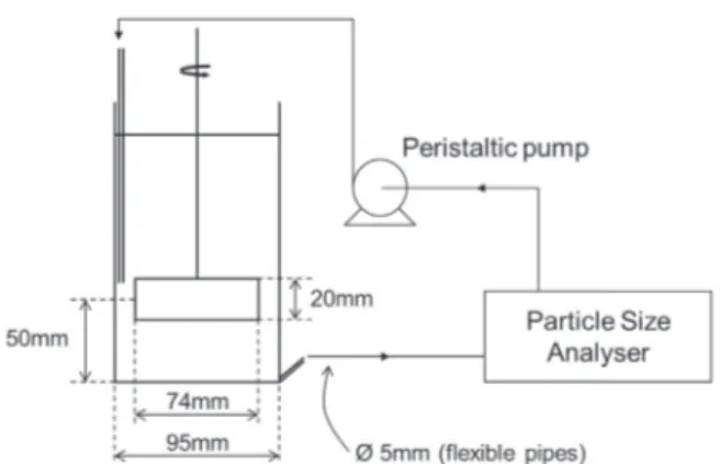
The experimental setup is sketched inFig. 1.

Flocculation experiments were conducted in a 1-L jar test vessel and monitored by on-line light scattering analysis. The hy-drodynamics in the reactor was studied by (Bouyer et al., 2001). The mean values of the most important hydrodynamic character-istics are presented inTable 1: N (rpm) is the tuned rotation speed of the impeller, Re (-) is the Reynolds number defined asRe=ND_ν2 where D (m) is the impeller diameter and ν(m2_s" 1_{) is the}

ki-nematic viscosity, G (s" 1_{) is the mean velocity gradient and η}

(m) is the mean value of the Kolmogorov microscale. All experi-ments were conducted under turbulent conditions.

Measurements of the volume-based size distribution of ag-gregates were performed with the particle size analyzer Mas-tersizer2000 (Malvern Instruments).

The particles used in this study were IDC™ monodispersed latex beads purchased from Life Technologies™ (median diameter 2.15 mm). These beads were perfectly convenient for the modeling framework presented in the next section. The critical coagulation concentration (CCC) given by the supplier was 1 mol L" 1_of

mono-valent cation. The suspension was destabilized by sodium chloride at a concentration of 1.3 mol L" 1 _{above the CCC, providing a liquid}

phase density equal to that of the solid phase (1055 kg m" 3_{) to}

avoid sedimentation. The viscosity measured at 25 °C was µ =₁₀−3

Pa.s; therefore, the hydrodynamics were unchanged by the presence of the salt. The water used was demineralized and degassed. The saline solution was first poured into the reactor. Then, the rotation speed and the circulation were set, and the latex beads were finally injected in an area close to the impeller to favor quick mixing. The solid volume fraction of the suspension was

φ

¼ 3.5 10" 5. All ex-periments were conducted at room temperature.

To monitor the evolution of the size distribution in the course of the experiments, which lasted 4 h, samples were continuously recycled after measurement so that the suspension volume re-mained constant. The tank was customized with a tangential outlet at the bottom, from which the suspension flowed toward the measurement cell through flexible pipes. A peristaltic pump located downstream of the measurement allowed draining of the

Fig. 1. Experimental apparatus.

Table 1

Main hydrodynamic properties in the jar test.

N (rpm) 60 90 150

Re (dimensionless) 5800 8700 14,000

G (s" 1_{) 34 65 133}

sampled suspension back into the tank, where it was reinjected in the impeller zone through a fixed solid pipe. All pipes were made as short as possible to minimize the residence time outside of the tank (o 20 s). The volume in the measurement loop was less than 5% of the total volume. The pump flow was chosen to provide a mean velocity gradient in the flexible pipes equal to the one in the tank. Thus, the changes in hydrodynamic conditions caused by the measurement and recycling loop were minimized, and their con-sequences were negligible for the purpose of this work.

2.2. Experimental results

According to Mie’s theory, the scattered light signal is inter-preted as a volumetric PSD using the diameters of equivalent

spheres, referred to as CED (Circle Equivalent Diameter). The vo-lume average value of the vovo-lume distribution as given by the particle size analyzer software is plotted in Fig. 2. As is well known, the average CED increases during flocculation (Oles, 1992). The resulting size increases as the shear rate decreases. Obviously, it also stabilizes faster when the shear rate is higher. Thus, a pla-teau was reached within the experimental duration only in the case of the highest shear rate.

The Particle Size Distributions (PSD) versus time are plotted in

Fig. 3 for each tested hydrodynamic condition. The PSD of the primary particles is represented as a continuous line and was measured without salt.

t0corresponds to the first measurement done during the

ex-periments, that is a few seconds after the injection of the particles in the jar. The mode of the PSD measured at t0is reported onFig. 4

as a function of the applied mean shear rate G. It can be concluded from this graph that the aggregation of the primary particles is rather rapid since aggregates are formed quasi-instantaneously and the aggregate size is controlled by the hydrodynamics even in the early stage process.

As the process time increases, the mode of the PSD increases as G decreases. As previously mentioned, thefloc size is correlated to hydrodynamics and especially to the mean shear rate G. This finding is in accordance with previous works (Bouyer et al., 2001,

2004). Moreover for _G=_{34 s}−1_{the size distributions are clearly}

bimodal, showing a main population constituted by large flocs and a second population corresponding to tiny aggregates. The spreading of the PSD is related to the heterogeneity of the hy-drodynamics in the mixing tank. Indeed, as shown byBouyer et al., 2004,2005, the more G is increased, the more homogeneous the mixing is and the more narrowed the distribution is. As a con-sequence, the full PSD is controlled by the hydrodynamics.

Looking more precisely on the volume based PSD versus time reported onFig. 3, it can be seen that the steady state seems to be reached at G¼133 s" 1 _{as the last two PSD are almost}

super-imposed, but the PSD for G¼34 s" 1_{was still evolving after 4 h of}

experiments. This point will be discussed in the later sections. Considering aggregates made of identical primary particles, the aggregate volume v and the aggregate size L are related through

:

= 34 s

-1

:

= 65 s

-11

:

= 133 s

-1

Fig. 2. Average value of the Circle Equivalent Diameter versus time for 3 hydro-dynamic conditions.

(a) G

G = 34 s

-1

: prima

: t

0

+ 1

(

ary particles

1 hour

(b) G = 65 s

-1

: t

0

+ 2 h

1

: t

0

ours

: t

0

+ 15 min

: t

0

+ 4 ho

(c) G = 13

n

ours

33 s

-1

the fractal dimensionDfdefined byEq. (1)where v0is the primary

particle volume and L0is the primary particle diameter (v0=Φ0 0L3

where Φ =π

0 ₆ in the case of spherical primary particles).

= ( ) ⎛ ⎝ ⎜ ⎞ ⎠ ⎟ v v L L 1 D 0 0 f

The fractal dimension is an indicator of the aggregate structure, its value ranges between 1 (linear) and 3 (spherical, non-porous particle).

Experimentally, it was possible to obtain global information about the particle structure by determining a scaling exponent or fractal dimensionDffrom the slope of a log-log plot of the relative

scattering signal I versus the modulus of the scattering wave vector q or the scattering angle in the power law regime (Spicer et al., 1998;Sorensen, 2001;Ehrl et al., 2008). Although our con-ditions do not fulfill the Rayleigh – Debye – Gans theory since the size of the primary particles is larger than the laser wavelength, it can be noticed that for the larger scattering angles there is only one single slope. Thus, the fractal dimension Df has been

ap-proximated to the scaling exponent that is the slope of the scat-tering plot for angles lying between 3° and 30°. During the first hour, the aggregates were only composed of a few primary par-ticles (as can be deduced fromFig. 2); therefore, the obtainedDf

values may not be relevant (Ehrl et al. (2008)). After the first hour,

Df remained almost unchanged over time so that constant values

of Df were imposed in the numerical part of the study

corre-sponding to the final values (after 4 h) of Df. Those values are

given inTable 2.

As shown byOles (1992) andSelomulya et al. (2001), Df

in-creases with the average shear rate. According to the previous authors, for very low shear stress, aggregates withstand the hy-drodynamic shear forces and show open structures. As the shear

stress increases, the restructuring of aggregates, most likely due to a more frequent exposure to the high shear zone near the impeller (Bouyer et al., 2005) is observed leading to more compact struc-tures and thus to higher values of Df.

As the modeling part of study will be performed with QMOM, it is necessary to compute the 6 moments of the PSD from the ex-perimental data. The particle size analyzer provides a volume fractionv L( ̅ )i of particles within a size range[L ; Li i 1+ ]represented

by the size Li̅, which is the geometric mean of the size range. The moment of order k of a size distribution is generally expressed as a function of the density functionn L t( , )as defined byEq. (2).

∫

( )

= ∞

( )

_{( )} m t L n L t dL, 2 k k 0

The conversion of v L( ̅ )i to the number density n L( ̅ )i was

per-formed accounting for Df as follows. By definition, the number

density can be expressed asEq. (3), where Niis the number (per

suspension volume unit) of aggregates in the size range[L ; Li i 1+ ].

( )

̅ = − ( ) + n L N L L 3 i i i 1 i

The number Nican be deduced from the volume occupied by

the particles in the size range divided by the representative vo-lume of this size rangeVi̅ (Eq. (4)),

( )

φ = ̅ ̅ ( ) N v L V 4 i i i

where

φ

is the volume fraction of particles. The representative

volumeVi̅ is related to the representative diameterLi̅ according to

the fractal relationEq. (1).

From the previous equations, the number density is obtained as

( )

̅ =

( )

₍

̅ φ

₎

Φ ̅ +− ( ) n L v L L L L 5 i i iDf i 1 i where Φ = Φ ( ) − L D 6 0 0 3 f

Finally, the experimental moments of the number distribution are evaluated as

(

)

( )

(

)(

)

∑

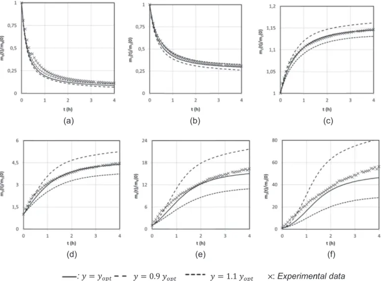
φ = − Φ − + ( ) ++ + + m v L L L L L L k 1 7 k exp i i ik ik iD i i , 1 1 1 1 f

To highlight the influence of the introduction of Df in the

ex-perimental moments, Fig. 5 shows the evolution of the experi-mental moments normalized by their initial value for the case

=

G 65s-1_{. The results are compared on each graph with the}

ex-perimental value Df=1.9to the one that would be obtained with the assumptionDf=3.Fig. 5shows that the sensitivity of the mo-ments to Df increases with their order and that the moments of

orderk<Dfdecrease over time while the moments of orderk>Df

increase. By definition, the zero-order moment is the total number of particles. As aggregation occurs, the total number of particles decreases (Fig. 5(a)). The first-order moment corresponds to the total size, which also decreases over time (Fig. 5(b)). Usually, when

=

Df 3, the 3rd order moment is related to the total mass (assuming a constant material density) and therefore is expected to be con-stant (Fig. 5(d)). Taking into account the fractal dimension for the computation of the experimental moments, the conservation of the total mass is verified for k=Df=2. WhenDf is close to 2, the

2nd order moment is thus almost constant (Fig. 5(c)). A focus on the largest particles of the population can be made with the mo-ments of order k≥3. Duringflocculation, aggregates grow over time leading naturally to an increase in the high order moments.

:

Mode of the PSD at t

0

: Mode of the PSD at t

f

1

10

100

10

100

1000

Si

ze

(µm)

G (s

-1

₎

Fig. 4. Characteristic sizes of the aggregates at t0and tf.

Table 2

Experimental values of Dfused in the model.

G (s" 1_{) 34 65 133}

Changing the fractal dimensionsDf to values other than 3

sig-nificantly changes the values and physical meanings of the mo-ments. The impact of the fractal dimension on the estimation of the usual ratios Dp q, defined by Eq. (8), which still have the

di-mension of the characteristic diameters, is now addressed.

= = + ( ) D m m ;p q 1 8 p q p q ,

The most current Dp q, are plotted onFig. 6. D1,0is the number

average diameter while D3,2and D4,3are interpreted as the surface

and volume average diameter, respectively, when the assumption =

Df 3is valid. As can be expected, Dp q, are higher when evaluated

with a lower Df. Indeed, a lower fractal dimension implies looser

aggregates that appear larger for a given amount of solid matter.

3. Population balance model

3.1. Introduction of the fractal dimension in a diameter-based po-pulation balance

The continuous population balance equation for aggregation and breakage in a homogeneous system describes the time

evolution of the number density of particle volume as Eqs.(9)–(13)

(Kumar and Ramkrishna, 1996), where ) v t′a

( )

, and ) v t′ (b , )are

the birth terms due to aggregation and breakage, respectively, and similarly + v t′a

( )

, and + v t′b

( )

, are the death terms due to

ag-gregation and breakage.

(

( )

)

_{( )}

_{( )}

_{( )}

_{( )}

∂ ′ ∂ = ′) − ′+ + ′) − ′+ ( ) n v t t v t v t v t v t , , , , , 9 a a b b

∫

( )

α

(

) (

)

′ = ′( − ) ′( − ) ′ − ′ _{( )} ) v t, 1 v u u C v u u n v u t n u t du 2 , , , , 10 a v 0

∫

( ) (

α

(

)

′ = ′ ) ∞ ′( ) ′( ) ′ _{( )} + v t n v t, , v u C v u n u t du, , , 11 a 0

∫

( )

β

(

)

′ = ∞ ′( ) ′( ) ′ _{( )} ) v t, v u B u n u t du, , 12 b v

( )

′ = ′( ) ′( ) ( ) + v t B v n v tb , , 13

In these equations, the prime symbol (′) indicates functions of particle volume; n v t′( , )is the number density of particles of vo-lume v at time t;C u v′( , )is the collision kernel (m3_s" 1_{) modeling}

the collision frequency of particles of volumes u and v; α′(u v, )is

(a)

(d)

(b)

(e)

:

= 1.9

:

= 3

9

(c)

(f)

Fig. 5. Influence of Dfon the changes of mk t( )_{( )}

mk 0 as a function of time for G¼65 s

the collision efficiency i.e., the rate of collisions that effectively lead to aggregation;B v is the breakage kernel representing the′( ) disruption frequency of a particle of volume v (s" 1_{) andβ′(v u, )is}

the fragment distribution function describing the number density of particles of volume v produced by the breakage of a particle of volume u. The aggregation and breakage functions are to be modeled according to physical considerations that depend on the experimental system and will be detailed in the next section.

The general aggregation-breakage equation (Eq. (9)) describes the evolution of the volume-based number density function and must fulfill the mass conservation constraint (or the volume con-servation if a constant particle density is considered). Indeed, whatever the type of event (aggregation or breakage), the mass (or the volume) of the parent aggregate(s) must be strictly equal to the mass of the daughter particle(s). It is possible to reformulate the population balance in terms of particle size (length), providing a relation between particle size and volume given by the fractal relation (Eq. (1)). The population balance is reformulated below as the evolution of the diameter-based number density function, involving the aggregate fractal dimension that is introduced by the conversion from volume to diameter. This formulation is a gen-eralization of the one proposed by (Marchisio et al., 2003a) that was written in the particular case Df=3; such a generalization to

≠

Df 3was suggested by (Wang et al., 2005).

Let the fractal dimension (Eq. (1)) be rewritten as Eq. (14)

where Φ=Φ_{0 0}L3−Df_{. Then, the relations between the differential}

quantities (Eq. (15)) are derived, and the relation between the volume-based number density functionn v t′( , )and the diameter-based number density functionn L t( , )are given asEq. (16).

Φ = ( ) v LDf 14 Φ Φ = ⟺ = ( ) − − dv D L dL dL dv D L 15 f D f D 1 1 f f

( )

_Φ

( )

′ = ( ) − n v t n L t D L , , 16 f Df 1

The collision frequency, the collision efficiency and the break-age kernels are then written as functions of sizes (L or λ) instead of volumes ( v or u, respectively) according to Eqs.(17)–(19).

(

Φ Φλ

)

λ ′( )= ′ = ( ) ( ) C v u, C LD_f, D_f C L, ₁₇

(

)

α′(v u, )= ′α ΦLDf,ΦλDf = (αL,λ) ₍18₎

(

Φ

)

′( )= ′ = ( ) _{( )} B v B LD_f B L ₁₉

The fragment distribution function is subjected to the same transformation as the number density function, leading toEq. (20).

β β λ Φ ′( )= ( ) ( ) − v u L D L , , 20 f Df 1

The diameter-based (or length-based) population balance equation is eventually obtained as Eqs. (21)–(25). Note that the term of birth due to aggregation ) L ta

( )

, involves a conversion from a volume difference ( − )v u to the corresponding length

λ (LDf − _{Df Df}) 1 .

( )

( )

( )

∂( ( )) ∂ =) −+ +) −+ ( ) ( ) n L t t L t L t L t L t , , , , , 21 a a b b

∫

( )

( )

λ λ λ λ λ λ = ( − ) ( − ) ( − ) ( ) − − ⎛ ⎝ ⎜ ⎞ ⎠ ⎟ ⎛ ⎝ ⎜ ⎞ ⎠ ⎟ ⎛ ⎝ ⎜ ⎞ ⎠ ⎟ ) L t L Q L n L t n t L d , 2 , , , 22 a D L D D D D D D D D D 1 0 1 1 1 ₁ f f f f f f f f f f

∫

( )

= ( ) ∞

(

λ

) ( )

λ λ _{( )} + L t n L t, , Q L, n ,t d 23 a 0

∫

( )

= ∞β

(

λ

) ( ) ( )

λ λ λ _{( )} ) L t, L, B n ,t d 24 b L

( ) ( )

= ( ) ( ) + L t B L n L tb , , 25

whereQ L,

(

λ

)

is the aggregation kernel defined as:

(

λ

)

= ( λ α) ( λ) ( )

Q L, C L, L, 26

In this work, a population balance equation that accounts for the aggregate structure through the fractal dimension Dfdirectly

introduced by the volume to length conversion is proposed without any additional hypothesis. A similar methodology can be conducted for the expression of agglomeration and breakage kernels.

3.2. Introduction of the fractal dimension in breakage and aggrega-tion kernels

3.2.1. Breakage model

The breakage kernelB L

( )

is the breakage frequency of particles of size L. Several expressions for this function were proposed in the literature, among which two main forms can be retained

=1,9

: D

1,0

: D

3,2 :

D

4,3

= 3

: D

1,0

: D

3,2 :

D

4,3 0 2 3

Fig. 6. Influence of Df on the changes of some characteristic diameters as a func-tion of time (G¼65 s" 1_).

(Marchisio and Fox, 2013): the exponential form (Delichatsios and Probstein, 1976; Kusters, 1991; Oles, 1992; Kusters et al., 1997;

Wang et al., 2005;Sang and Englezos, 2012) and the power law kernel (Valentas et al., 1966; Ramkrishna, 1974; Pandya and Spielman, 1983; Wang et al., 2005; Marchisio et al., 2006; Soos et al., 2006;Soos et al., 2007). The latter is generally expressed as

( )

= B L C LC

1 2where C1and C2are constants. The first parameter C1

usually includes hydrodynamic characteristics as C G∝ C

1 3 (Wang

et al., 2005; Marchisio et al., 2006; M. Soos et al., 2007) or vε ν

C C C

1 4 5(Kramer and Clark, 1999;Marchisio et al., 2003b). In the

present study, the breakage frequency was expressed as

( )

= ( ) ⎛ ⎝ ⎜ ⎞ ⎠ ⎟ B L aG L L 27 b c 0

where a and bare adjusted parameters and c=D₃f+ −3 Df. The

physical meaning of this exponent is to be understood as follows. According to the fractal relation (Eq. (1)),

( )

L

L D_f

0 is proportional to

the solid volume; consequently,

( )

_LL D /3f

0 is proportional to the

diameter of the mass-equivalent sphere. The ratio

⎛ ⎝ ⎜ ⎞ ⎠ ⎟ ⎛ ⎝ ⎜ ⎞ ⎠ ⎟ L L Df L L 0 0 3 is the solid

volume divided by the circumscribed sphere volume so it can be interpreted as a density (Oles, 1992). Therefore,

⎛ ⎝ ⎜ ⎞ ⎠ ⎟ ⎛ ⎝ ⎜ ⎞ ⎠ ⎟ L L L L Df 0 3 0 can be in-terpreted as the inverse of density. The breakage kernel for-mulated here shows a dependence on the hydrodynamics re-presented by the mean shear rate and a double dependence on the aggregate properties: on the one hand a characteristic length re-presentative of the aggregate mass (the larger the aggregate, the more likely to break), on the other hand, a structure property re-presentative of the density (the looser the aggregate, the more likely to break).

A breakage event represents the splitting of an aggregate into smaller aggregates assuming mass conservation. The fragmenta-tion distribufragmenta-tion describes how the mass is distributed over the daughter particles. Among the most currently applied distribution functions (see, e.g., Marchisio et al., 2003a), one can find either some particular mechanisms such as symmetric fragmentation or erosion or continuous functions such as the uniform distribution of daughter particles. With no physical assumption on a specific breakage mode, a uniform fragmentation distribution was used in this work, meaning that all possibilities are equally probable. When the particle volume is used as an internal coordinate, it is expressed asEq. (28)(Kumar and Ramkrishna, 1996).

β′(v u)= < _{( )}

u v u

, 2,

28 To be used in a diameter-based population balance, the pre-viously mentioned conversion (Eq. (20)) is applied, leading toEq. (29).

(

)

β λ λ λ ′ L, =2D L − ,L< _{( )} 29 f D D 1 f f 3.2.2. Aggregation model

The aggregation kernel Q L,( λ)describes the aggregation fre-quency between two particles of given sizes L and λ and involves the collision frequencyC L,

(

λ

)

and the collision efficiency α

(

L,λ

)

. Several expressions of the collision frequencyC L,

(

λ

)

can be found depending on the aggregation regime considered that a relative velocity between particles must exist to allow their collision. It can

result from Brownian (diffusion) motion, differential sedimenta-tion or shear flow. In this work, when the primary particle dia-meter is 2.15 mm, the Peclet number that compares the Brownian diffusion time⎜⎛ πμ

( )

θ⎟ ⎝ ⎞ ⎠ k 6 L₂ / B 3

to the time scale of shear flow

(

1/G

)

is high (above 150), indicating that the Brownian motion is neg-ligible (Cloitre, 2010). The differential sedimentation was reduced by setting the fluid density equal to the solid one through the choice of salt concentration. Therefore, the relative motion of the aggregates is mainly due to fluid velocity gradients. In this case, with the aggregates being smaller than the Kolmogorov micro-scale, a classical orthokinetic kernel written asEq. (30)was cho-sen, where

(

L+λ

)

is the diameter of the collision sphere and G stands for the mean shear rate.

(

λ

)

=

(

+λ

)

( )

C L, G L

6 30

3

The collision efficiency is usually introduced as a correction factor, accounting for the fact that the aggregation frequency is actually lower than the collision frequency (Adachi et al., 1994). Therefore, the collision efficiency can be understood as the ratio of collision events leading to aggregation events. It can be used as a fitting parameter (Soos et al., 2006) thus independent from the sizes of the aggregating particles. However, many authors worked on establishing collision efficiency models based on physical considerations.

The curvilinear approach (Han and Lawler, 1992) was devel-oped as a complement to the rectilinear approach that led to the aggregation kernel expression, based on isolated particle trajec-tory calculations (Adachi et al., 1994). When two particles en-counter each other, hydrodynamic interactions induce trajectory modifications. Some authors studied the trajectories of two iden-tical solid spheres approaching one another (Van de Ven and Hunter, 1977). Adler addressed the issues of the sizes (Adler, 1981b) and permeability (Adler, 1981a) of particles. By calculating trajectories of impermeable solid spheres of different sizes, it was shown that homocoagulation is generally more favorable than heterocoagulation, i.e., the more different the particle sizes are, the less efficient the collision will be. Considering aggregate perme-ability, the flow penetration into the aggregate reduces the pre-viously mentioned trajectory modifications. Torres et al. (1991)

andKusters et al. (1997)proposed accounting for a potential floc porosity to evaluate the aggregation efficiency. Kusters et al. (1997) distinguished three cases: solid (nonporous) particles, porous impermeable flocs and porous permeable flocs, with por-osity being represented by a fractal dimension. The latter are de-scribed by the shell-core model, representing a solid core whose radius is used for the trajectory calculation, surrounded by a permeable shell used to evaluate the collision radius. Collision efficiency in each of these three cases was evaluated as a function of the size ratio between the two particles. The results from this set of calculations offered a strong dependence of the collision efficiency on the structure (porosity) and the sizes.Selomulya et al. (2003)thereafter proposed a collision efficiency model given by

Eq. (31).

(

)

α λ=α − − ( ) ( ) ⎜ ⎟ ⎛ ⎝ ⎜ ⎛_⎝ ⎞_⎠⎞ ⎠ ⎟ L exp x n n , . 1 . 31 max n n i j y 2 i j

In this expression, the aggregate size is expressed as a mass, represented by the number of primary particles composing the aggregates, niand njdefined as

(

λ

)

(

λ

)

= = ( ) ⎛ ⎝ ⎜⎜ ⎞ ⎠ ⎟⎟ ⎛ ⎝ ⎜⎜ ⎞ ⎠ ⎟⎟ n min L L n max L L , ; , 32 i D j D 0 0 f f

The efficiency collision involves three parameters αmax,xand y. The collision efficiency is all the more high when aggregates are small, which is reflected by the product n ni jand the parametery.

The maximum value of

α

is reached when two primary particles

encounter ( = =n n 1i j ) and is equal to a third adjustable parameter

αmax (ranging between 0 and 1). In this study, the NaCl

con-centration being above the CCC, the energy barrier is thus com-pletely overcome, and it can be thought that the aggregation of primary particles will always be successful. Therefore, the max-imum efficiencyαmaxwas set to 1. Moreover,

α

is higher when the

colliding aggregates have similar sizes, leading to a preference of homocoagulation versus heterocoagulation. This is accounted for by the ratio n ni/ j and the parameter x. This partially empirical

model was shown to adequately simulate latex flocculation ( Se-lomulya et al., 2003; Bonanomi et al., 2004; Soos et al., 2007;

Antunes et al., 2010;Jeldres et al., 2015).

In the present work, the collision efficiency model proposed by Selomulya et al. (Eq. (31)) was considered. The fractal dimension was used to evaluate the number of primary particles (Eq. (32)). The collision efficiency was therefore calculated in such a way that a dependency on the aggregate structure was considered. The parameters x andywere adjusted to fit the experimental data (see

section 4.1, x=0.014 and y=0.6). The resulting values of the collision efficiency for homocoagulation (L1=L2) used in the

pre-sent model are plotted inFig. 7for different values ofDf. The range

of sizes corresponds to those of the experiments (Fig. 3). The collision efficiency is maximum for the collision of primary par-ticles (α

(

L0,L0

)

=αmax=1) and sharply decreases as the size of ag-gregates increases.

In the case of heterocoagulation,Fig. 8illustrates the isovalues of α

(

L,λ

)

. The graphs are obviously symmetrical because

(

)

α L,λ= (α λ,L). The aggregation efficiency values for homo-coagulation are located on the first bisector. The higher values are obtained in the bottom left corner of the graphs because this lo-cation corresponds to homocoagulation between primary parti-cles. The fast decreasing of α(L,λ)with increasing sizes is due to the high weighty, while the shape of the lines depends on the pair of parameters (x y, ). Due to the adjusted parameters, a much higher weight is given to the mass product ( =y 0. 6 than to the) mass ratio ( =x 0. 014). The iso-lines are therefore perpendicular to the first bisector over a wide region, where the mass ratio has practically no influence (this trend is observed when y is sig-nificantly higher than x, whatever their absolute values). If a re-latively higher weight was set to the size ratio, the lines would be shaped as more elongated lobes. The difference between the three graphs ofFig. 8is solely due to the fractal dimension. When Df

increases, the number of primary particles in an aggregate of a given size also increases so the aggregation efficiency decreases. Therefore, the aggregation efficiency values for fractal aggregates are much higher than those of spherical particles.

In the present model, α(L,λ)varies by three orders of magni-tude in the experimentally covered size range, indicating a very strong dependency on the size. It was indeed impossible to fit the experimental data with a constant value of the collision efficiency. For the fractal dimension, the influence of the collision efficiency is also noticeable: more porous particles aggregate more easily. 3.3. Moment transformation

The Quadrature Method of Moment (QMOM) is based on the quadrature approximation (Eq. (33)) (McGraw, 1997) where w ti( ) is the weight associated with the abscissa L ti( ), leading to the moment approximation (Eq. (34)).

( )

≈

∑

( ) ( − )δ ( ) = n L t, w t L L 33 i N i i 1 q : =1,7 : ==1,9 : =1,95 : =3 Fig. 7. Collision efficiencyα

(

L L,

)

for 4 values ofD xf

₍

=0.014;y=0.6

₎

.

Fig. 8. Iso-values of the collision efficiencyα_α(L L) max

1, 2 _{obtained with different values ofD x}

₍

_=0.014;y=0.6

₎

Table 3

Overview of the aggregation-breakage model. Aggregation model

( )

( )

(

)

(

)

α = = + − − ( ) ⎛ ⎝ ⎜ ⎜ ⎜ ⎜ ⎜ ⎜ ⎜ ⎛ ⎝ ⎜ ⎜ ⎜ ⎜ ⎜ ⎜⎜ ⎞ ⎠ ⎟ ⎟ ⎟ ⎟ ⎟ ⎟⎟ ⎞ ⎠ ⎟ ⎟ ⎟ ⎟ ⎟ ⎟ ⎟ ⎛ ⎝ ⎜ ⎞ ⎠ ⎟ ⎛ ⎝ ⎜ ⎜ ⎜ ⎞ ⎠ ⎟ ⎟ ⎟ ⎛ ⎝ ⎜ ⎜ ⎜ ⎞ ⎠ ⎟ ⎟ ⎟ Q Q L L G L L exp x , 6 . 1 37 ij i j i j max min Li Lj L Df max Li Lj L Df LiLj L Dfy 3 , 0 , 0 2 02

Breakage model Breakage frequency

( )

= = ( ) − ⎛ ⎝ ⎜ ⎞ ⎠ ⎟ B B L aG L L 38 i i b i D f 0 3 2 3

Fragment distribution (moment)

β ̅= + ( ) L D k D 2 39 ik ik f f

Fig. 9. Time evolution of normalized experimental and numerical moments for G ¼65 s" 1_{( D}

( )

≈

∑

( )

( ) ( ) = m t w t L t 34 k i N i _i k 1 q

where Nqis the order of the method.

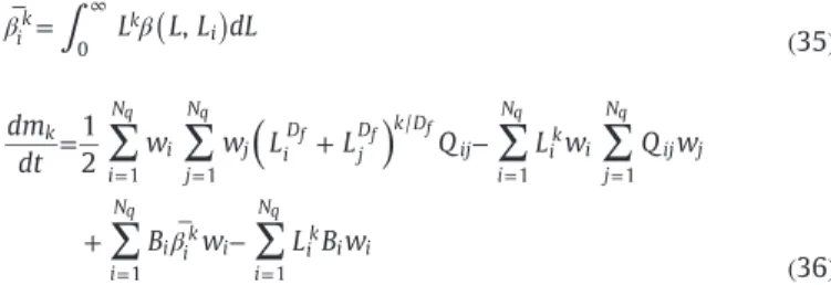
Implementing the moment approximation in the continuous PBE (Eq. (21)), the discretized moment equations are finally ob-tained (Eq. (36)) where β ̅i

k_{is the k}th

order moment of the fragment distribution function:

∫

(

)

β̅ = β ( ) ∞ L L L dL, 35 i k k i 0

(

)

∑

∑

∑

∑

∑

β

∑

= + − + ̅ − ( ) = = = = = = dm dt w w L L Q L w Q w B w L B w 1 2 36 k i N i j N j i D j D k D ij i N ik i j N ij j i N i ik i i N ik i i 1 1 / 1 1 1 1 q q f f f q q q q

The expressions of the aggregation ( Qij) and breakage (Biand β ̅_ik) kernels used in this study are summarized inTable 3.

The numerical resolution of the moment equations (Eq. (36)) is accomplished by using the product-difference algorithm (Gordon, 1968; Marchisio et al., 2003b). The QMOM with order N 3q= was proven accurate for aggregation-breakage problems (Marchisio et al., 2003a). It allows following the evolution of the first six moments of the distribution.

4.1. Numerical methods and results

The QMOM was implemented in Matlab using three nodes to reproduce the evolution of the first six moments of the size dis-tribution as a function of time. The initial conditions of the six moments were obtained through the experimental measure after the injection of particles into the jar test. The numerical solution required the adjustment of four parameters a, b, x and y. The first step of the simulation consisted of focusing on the early stage of flocculation when mainly agglomeration occurred. Indeed, be-cause the flocs were tiny, they were not subjected to rupture, and the breakage terms of the PBE were small compared to the ag-glomeration ones and could thus be neglected. By assuming that a and b were equal to zero at the beginning of the process, ap-proximate values of parameters x and yincluded in the agglom-eration efficiency could be determined. x and ymainly influenced the slope of the exponential growth stage (not shown here). In a second step, keeping x and yfixed, the parameters a andbwere adjusted to handle the steady-state moments. Because breakage mainly impacts large aggregates, this fitting was mostly performed on the high order moments ( k Z 3). To support the above meth-odology,Fig. 9 illustrates the change in the first six normalized moments versus time. Here, the values derived from the experi-mental data and the simulated ones are compared taking into

Fig. 10. Change over time of normalized experimental and simulated moments for G ¼34 s" 1_{( D}

f¼ 1.75).

account or ignoring the breakage terms. During approximatively the first hour of the process, the experimental moments are equally fitted with or without the breakage events but the gap is increasing then more and more if the rupture is neglected. From a general point of view, as expected, the larger a andbare, the more rapidly the steady-state moments are reached.

After these two preliminary steps, a set of optimized fitting parameters was obtained through a Matlab function of optimiza-tion based on minimizing differences between the six experi-mental and numerical moments. Finally, the set of optimized fit-ting parameters was

= = = = − − ⎧ ⎨ ⎪ ⎪ ⎩ ⎪ ⎪ ⎪ ⎫ ⎬ ⎪ ⎪ ⎭ ⎪ ⎪ ⎪ a e s b x y 2 2,5 0,014 0,6 opt b opt opt opt 10 _opt1

InFigs. 10–12, the evolutions of the six moments normalized by their initial value are plotted against time for the three mean shear rates experienced.

Whatever the shear rate, the parameters enabled fitting the order of magnitude of the experimental data. The special feature of the experimental results was their very slow evolution. The higher the k, the lower the G, and the slower the evolution of the size. For G ¼133 s" 1_{; low order moments quickly reached a plateau. In}

contrast, for G ¼34 s" 1_{, the six moments were still evolving after}

4 h. This behavior was particularly difficult to model. The first si-mulations were drawn using a constant but adjustable efficiency,

coupled with various models of breakage; all failed to reproduce this slow dynamics. Indeed, most of the models "naturally" brought a relatively fast evolution towards a steady state. Taking into account the sizes and the ratio between the sizes of the ag-gregates colliding, only the model of Selomulya was able to cor-rectly reproduce this slow evolution of moments, with different dynamics according to the velocity gradient. Fitting the six mo-ments allows the behavior of the entire population to be tracked. However, from a numerical point of view, it was rather proble-matic to reach a satisfying fit for each of the six moments.

More generally, numerical model predictions are validated considering the changes versus time of some characteristic aver-age sizes such as D1,0or D4,3. The values of D1,0, D3,2, and D4,3

derived from the experimental data or calculated using the model with the optimized set of parameters are reported inFig. 13.

The characteristic average sizes were quite satisfactory but re-mained less correctly predicted than the six moments of the dis-tribution. From a general point of view, the evaluations of D1,0was

of the right order of magnitude but the precision was lower than expected, most likely due to the conversion in the number of the native volume distribution. Predictions of D3,2and D4,3look better.

However, because the size volume distributions were mostly bi-modal, global parameters such as Dp q, do not correctly represent

the entire population. 4.2. Precision of the model

To quantify the precision of the model, the Goodness of Fit (GoF) used by several authors (Biggs and Lant, 2002; Antunes Fig. 11. Change over time of normalized experimental and simulated moments for G ¼65 s" 1_{( D}

Fig. 12. Change over time of normalized experimental and simulated moments for G ¼133 s" 1_{( D}

f¼ 1.95).

et al., 2010; Jeldres et al., 2015) was adapted and calculated. In-deed, GoF was calculated including the 6 moments of the size distributions without giving weight to one moment k over an-other.

( )

=

∑

̅ −σ ̅ ( ) = GoF m m % 100. 40 k k k k 0 5

where mk_̅ is the average of all the data values over the process

time and σkis the standard error.

A GoF of 100% would represent a perfect fit of the model to the experimental results for the six moments of the distribution. With the set of fitting parameters presented above, the global GoF was determined to be greater than 85% as seen inTable 4.

The quality of the fitting was higher for the moments of order 1–4 than for m0and m5in accordance withFigs. 10–12. This

in-dicates that the model provides a rather good estimate of the flocculation dynamics.

4.3. Sensitivity analysis

By varying the 4 parameters independently, a first sensitivity analysis of the model can be drawn. The influence of each para-meter on the GoF is shown on Fig. 14 for the 3 experimental conditions. The plotted values of GoF were obtained by varying one parameter by approximately 20% of its optimized value, while the three other were kept constant.

Whatever the shear rate, the GoF displays similar tendencies.

Fig. 14shows a higher sensitivity of the model to band y com-pared to a and x in the vicinity of the optimized values. This can be understood from a mathematical point of view. Indeed, regarding the breakage kernel (Eq. (27)), a is a multiplying factor whilebis an exponent. Regarding the aggregation efficiency (Eq. (31)), both x and yare exponents, but the value of ybeing much higher than

x makes the 20% variation of x poorly significant. Thus, by keeping a and xfixed to aoptand xopt, a more detailed sensitivity analysis

can be drawn.Fig. 15provides the sensitivity analysis on moment predictions for values of bvarying by 10%.

The parameter b played an important role mainly over the moments of high order ( k 42), that is, on rather large particles (Fig. 15(c)–(f)). This effect was all the more important as G was high (not shown in the figures). An increase ofbfavored breakage events, thus the moments of high order were lower forb=1.1bopt

leading to smaller aggregates and thus a higher number of parti-cles in the entire population. Indeed, the higherbwas, the higher m0and m1were. The parameter balso played a role in the time

needed to reach the steady state: the higherbwas, the quicker the steady state seemed to be reached.

Fig. 16presents a similar sensitivity analysis for y.

Increasing yled to a reduction in the agglomeration efficiency, specifically the higher the sizes of the colliding aggregates, the lower αis. Therefore, as yincreased, m0and the total length (m1)

slightly increased whereas moments of orders higher than 2 de-creased meaning that formed flocs are less numerous and smaller (Fig. 16(a) and (b)). To better understand their sensitivities, the analysis of each of the 4 terms of the PBE is performed in the next section.

4.4. Evolution of source and sink terms of the PBE

The time evolution of the moments of the distribution brings in four terms; for each phenomenon (agglomeration and breakage), both a sink (or death) and a source (or birth) term are involved as shown inEq. (41). = − + − _{( )} dm dt B D B D 41 k a a b b

The change over time of each term of the PBE is shown in

Fig. 17.

For the first two moments (m0andm1), the agglomeration sink

term is dominant compared to the agglomeration source term (Fig. 17(a) and (b)). This can be explained by the facts that (1) small particles are numerous and (2) their collision efficiency is high (Fig. 8). The breakage terms behave just the opposite and are nearly constant. As expected at the beginning of the experiment, the weights of the agglomeration terms were high compared to those of the breakage terms, validating the way we conducted the first step in the research of fitting parameters. Surprisingly, at the end of the experiment, the agglomeration source term was close to

Fig. 14. Evolution of GoF. Table 4 GoF values. m0 m1 m2 m3 m4 m5 G ¼34 s" 1 _{GoF of m} i 72.6 92.4 98.3 91.9 88.3 85.6 Global GoF 88.2 G ¼65 s" 1 _{GoF of m} i 81.9 95.1 99.7 96.5 91.0 77.7 Global GoF 90.3 G ¼133 s" 1 _{GoF of mi 72.7 86.6 99.4 89.7 86.3 76.8} Global GoF 85.25

the breakage sink term, and the agglomeration sink term was al-most equal to the breakage source term (Fig. 17).

For moments of high order (m3to m5), the agglomeration terms

dominated the breakage terms at the beginning of the process (Fig. 17(c)–(f)). At the beginning of the experiment, because the population was mainly composed of small particles that were not much subjected to breakage, the weights of breakage terms are negligible. As time t increases, the flocs grew leading to an in-crease of in the rupture frequency and thus of the source and sink breakage terms.

For any the order of the moment ( k),Fig. 17shows that both breakage terms seemed to behave the same way. From a mathe-matical point of view, the ratio of breakage terms reads:

( )

( )

=∑ ∑ = + = ( ) = + − = − B D L a G w L a G w D k D cste . . . . . 2 . 42 b b i N ik D k D b L L i i N ik b L L i f f 1 2 . 3 1 3 q f f i Df q i Df 0 2 3 0 2 3

Thus, regardless of the size of the aggregate, the ratio between the two breakage terms only depends on the order of the moment (k). WhenDfis close to 2, for k o2, Bb4Db, while if k Z2, BboD_b. This result can be extended to most of the frequency kernels and fragment distribution functions. Among the various forms of the fragmentation function, only the erosion kernel does not lead to a constant ratio of the breakage terms.

The behavior of the agglomeration terms of the PBE was less obvious than that of the breakage terms. Indeed, the ratio of the agglomeration terms of the PBE could not be written as easily as that of the breakage terms. However, the following developments could be applied for any type of agglomeration kernel (Qij).

In the case of moment of order 0 (k ¼0),Eq. (36)becomes

∑

∑

∑

∑

∑

β

∑

= − + ̅ − ( ) = = = = = = dm dt w w Q w Q w B w B w 1 2_{i 43} N i j N j ij i N i j N ij j i N i ik i i N i i 0 1 1 1 1 1 1 q q q q q q

From which the following relations can be derived:

= _{( )} B 1D 2 44 a a = ( ) Bb 2Db 45

At steady state conditions, assuming the previously established relation between breakage terms (Eq. (42)),

= ( )

Ba Db 46

= ( )

Da Bb 47

From a physical point of view, Eq. (46) indicates that the number of aggregates smaller than a size L involved in aggregation events leading to the birth of an aggregate of size L is strictly

Fig. 15. Sensitivity analysis for parameter b: change over time for G ¼65 s" 1_{of normalized experimental and numerical moments ( D}

balanced by the number of daughter particles produced by the breakage of particles of size L.Eq. (47)means that the number of aggregates of size L involved in agglomeration phenomena leading to aggregates with size greater than L is equal to the number of daughter particles produced by the breakage of particles larger than L.

From a practical point of view, the previous relationsEqs. (46)

and(47)show beyond a doubt that for a shear rate of 65 s" 1_{, the}

steady state was not completely reached after 4 h of flocculation (Fig. 17(a) and (b)).

For higher order moments ( k 40), writing the agglomeration terms in matrix form as

∑

= ( ) ⎡ ⎣ ⎢ ⎢ ⎢ ⎢ ⎤ ⎦ ⎥ ⎥ ⎥ ⎥ D w L Q w w L Q w w L Q w w L Q w L Q w w L Q w w L Q w w L Q w L Q . . . . . . . . . . . 49 a k k k k k k k k k 12 1 11 1 2 1 12 1 3 1 13 2 1 2 21 22 2 22 2 3 2 23 3 1 3 31 3 2 3 32 32 3 33

whereQij=Qji, the following relationship between diagonal terms

arises:

( )

= −

( )

( ) Diag Ba 2 Diag D 50 k D a 1 f

However, the non-diagonal terms can only be easily linked in specific cases where there exists a relationship between

(

Li +L

)

D j D k D/ f f f_and

(

_{L +L}

)

ik kj .

(

)

(

)

(

)

(

)

(

)

(

)

(

)

(

)

( )

∑

= + + + + + + ( ) ⎡ ⎣ ⎢ ⎢ ⎢ ⎢ ⎢ ⎢ ⎢ ⎤ ⎦ ⎥ ⎥ ⎥ ⎥ ⎥ ⎥ ⎥ B w L Q w w L L Q w w L L Q w w L L Q w L Q w w L L Q w w L L Q w w L L Q w L Q 1 2 . 2. . . . . . . 2. . . . . . . 2. . 48 a D Dk D D Dk D D Dk D D Dk D Dk D D Dk D D _Dk D D _Dk D _Dk 12 1 11 1 2 1 2 12 1 3 1 3 13 2 1 2 1 21 22 2 22 2 3 2 3 23 3 1 3 1 31 3 2 3 2 32 32 3 33 f _f f f _f f f _f f f _f f _f f f _f f f f f f f f f

Fig. 16. Sensitivity analysis for parameter y: change over time for G ¼65 s" 1_{of normalized experimental and numerical moments ( D}

For monomodal particle size distributions ( = =L L L1 2 3), the

non-diagonal terms behave as non-diagonal terms, thus giving

= − ( ) Ba 2 D 51 k D a 1 f

In other specific cases, such as k=Df=2, then the agglomera-tion terms are equal to the breakage terms

= ( )

Ba Da 52

= ( )

Bb Db 53

ForG=65s−1_,D

fwas found to be equal to 1.9, which is close to

2, and it is the reason why the agglomeration and breakage terms seem to blend when approaching the steady-state inFig. 17(c).

5. Conclusion

A population balance model was adapted to describe the ag-gregation and breakage of fractal aggregates under varying tur-bulent conditions. The population properties were monitored thanks to an on-line experimental setup providing the change over

time of the volume-based distribution of an equivalent size (CED) and a fractal dimension. Using the fractal relation between ag-gregate mass and size, the experimental data can be interpreted as the number distributions, and their moments can be calculated. The interpretation of the moments, and particularly of their characteristic diameters ( D1,0,D3,2 and D4,3), was shown to be

different from usual when the assumption of spherical particles (Df=3) is not made. The fractal relation was then considered to transform the PBE, initially written as the evolution of the number distribution of particle volume, reformulated as the evolution of the number distribution of particle diameter. This formulation now accounts for the fractal dimension. The aggregation and breakage models were chosen depending on the hydrodynamic conditions through the mean shear rate G and on the aggregate structure throughDf. Moreover, the choice was made to adjust the

model parameters by fitting the moments instead of the char-acteristic diameters Dp q, because the moments are raw properties

of the distribution that contain more information about the po-pulation of aggregates than the characteristic diameters. The ex-perimental results obtained under various hydrodynamic condi-tions were adequately simulated by a single model (involving a single set of adjusted parameters), proving the relevance of the

Fig. 17. Change over time of source and sink terms for G ¼65 s" 1_{( D}