OATAO is an open access repository that collects the work of Toulouse
researchers and makes it freely available over the web where possible
Any correspondence concerning this service should be sent
to the repository administrator:
[email protected]
This is a publisher’s version published in:
https://oatao.univ-toulouse.fr/
2
6050
To cite this version:
Quintero Rincon, Antonio and D'Giano, Carlos and Batatia, Hadj A quadratic linear-parabolic model-based EEG classification to detect epileptic seizures. (2020) The Journal of Biomedical Research, 34 (3). 203-210. ISSN 1674-8301 . .
Official URL:
https://doi.org/10.7555/JBR.33.20190012
A quadratic linear-parabolic model-based EEG classification to
detect epileptic seizures
Antonio Quintero-Rincón
1,2,✉, Carlos D'Giano
1, Hadj Batatia
21Epilepsy and Telemetry Integral Center, Foundation for the Fight against Pediatric Neurological Disease, Montañeses 2325, Buenos Aires C1428AQK, Argentina;
2Computer Science Research Institute of Toulouse–National Polytechnic Institute of Toulouse, University of Toulouse, Toulouse, Cedex 7 B.P. 7122-31071, France.
Abstract
The two-point central difference is a common algorithm in biological signal processing and is particularly useful in analyzing physiological signals. In this paper, we develop a model-based classification method to detect epileptic seizures that relies on this algorithm to filter electroencephalogram (EEG) signals. The underlying idea was to design an EEG filter that enhances the waveform of epileptic signals. The filtered signal was fitted to a quadratic linear-parabolic model using the curve fitting technique. The model fitting was assessed using four statistical parameters, which were used as classification features with a random forest algorithm to discriminate seizure and non-seizure events. The proposed method was applied to 66 epochs from the Children Hospital Boston database. Results showed that the method achieved fast and accurate detection of epileptic seizures, with a 92% sensitivity, 96% specificity, and 94.1% accuracy.
Keywords: two-point central difference, curve fitting, parabolic curves, epilepsy, electroencephalogram, random
forest
Introduction
Epilepsy is a neurological disease that affects people of all ages. It is characterized by unpredictable seizures resulting from the hyperexcitability of neurons. The electroencephalogram (EEG) is the predominant modality to study cerebral activity. The analysis of EEG signals is nearly completely dependent on visual inspection by the physician to quantify or qualify the morphology of waves. Their goal is the identification and classification of abnormal patterns in order to provide aid for an
epilepsy diagnosis.
This study proposes a simple, fast, and adaptable method, implementable in real-time, to help physicians visually inspect EEG signals for epileptic seizure detection. The proposed method fits within the framework of model-based classification. It is based on the statistical parameters obtained from fitting a quadratic parabolic model to specifically filtered and transformed EEG signals. Precisely, the two-point central difference algorithm is used to build a filter for the EEG signals. The filtered signal is subsequently represented using a quadratic linear-parabolic model,
✉Corresponding author: Antonio Quintero-Rincón, Epilepsy and Telemetry Integral Center, Fight Against Child Neurological Dis-eases Foundation, Montañeses 2325, Buenos Aires C1428AQK, Argentina. E-mail: [email protected].
Received 16 January 2019, Revised 12 April 2019, Accepted 03 June 2019, Epub 28 August 2019
CLC number: R742.1, Document code: A The authors reported no conflict of interests.
This is an open access article under the Creative Commons Attribu-tion (CC BY 4.0) license, which permits others to distribute, remix, adapt and build upon this work, for commercial use, provided the original work is properly cited.
Open Access at PubMed Central
The Journal of Biomedical Research, 2020 34(3): 203–210 Original Article
using the curve fitting approach. Four statistical parameters are then calculated to characterize the model fitting. These parameters are considered as a feature-vector in the classification stage.
The literature abounds with research work dealing with the detection of epileptic seizure onset. Various methods and techniques have been proposed for this purpose. Many existing methods fit within the large framework of the feature-based machine learning approach.
The two-point central difference algorithm has proven useful in analyzing physiological signals, with various medical applications reported in the literature. A typical work has been reported by Frei et al to detect epileptiform discharges in muscles in EEG signals[1]. This algorithm is usually used to estimate
the derivative of a function, giving an estimate valid only over a limited frequency range. Here, our idea was to use this algorithm to design a filter that enhances the frequency range of EEG signals corresponding to brain activity characteristic of epileptic seizures. To single out the related waveform, we transform the filtered signal into a quadratic form. A quadratic linear-parabolic model is then fitted to the transformed signal, using the curve fitting technique[2–3].
The fitting is assessed using four statistical parameters (weighted sum of squared residuals, R-square, adjusted R-square, and root mean squared error). In order to show that our quadratic linear-parabolic model is pertinent to characterize epileptic seizures, we develop a classification method where the model-fitting parameters are used as features. We show that these features are good biomarkers of epileptic seizures.
The curve fitting technique adopted here is widely used in signal processing in general, and biomedical applications in particular. It has also been applied a few times in the domain of EEG and epilepsy. Orhan et al used the polynomial curve fitting method to fit a probability density function (PDF) of EEG signals discretized using equal frequency binning. The method has been applied to epileptic seizure detection using the comparison of PDFs of seizures and non-seizures. Second-order Fourier curve fitting has been used to smooth EEG signals in a pre-processing stage of a model-based method to predict epileptic seizures[4]. A spline curve fitting to EEG data was
proposed to detect phase cone patterns to characterize epileptic activity[5]. Linear curve fitting was applied to
interictal heartbeat intervals in order to combine EEG and ECG signals with the purpose of characterizing modulation patterns in patients with drug-resistant epilepsy[6]. More recently, a first-order exponential
function has been fit to voltage-gated sodium channel type 2 to model the conductance-voltage curves in
neonatal epileptic subjects[7].
Supervised machine learning methods have been widely used to detect seizures in EEG, with support vector machine (SVM) and K-Nearest Neighbor (KNN) being the most popular. SVM classifiers have been used with various features extracted from spectral and entropy analysis[8], matching pursuit
algorithm[9], tensor discriminant analysis[10],
multifractal detrended fluctuation analysis[11], and
cross-bispectrum analysis[12]. While KNN classifiers
have been developed, among many others, with features from the fractal dimension[13], and non-linear
dimension reduction of frequency domain
parameters[14]. In addition to these two popular
approaches, Acharya et al have recently been the first to develop a seizure detection method using a convolutional neural network[15].
In general, these methods have good performance thanks to the advanced signal processing techniques they rely on. However, they consequently have high computational costs[16]. In this work, we combine for
the first time the two-point difference algorithm and the quadratic linear-parabolic model to design an original model-based statistical classification method to detect epileptic seizures in EEG. The proposed feature-vector is simple and fast to calculate from the quadratic model. Our classification method is based on bootstrap-aggregated (bagged) decision trees. This approach combines results from several decision trees to overcome the overfitting effect due to the variability in the training data[17]. Using the different
subset of features (subspace sampling) to build the weak-tree classifiers reduces the training time[18], and
there are some recent works in seizure classification using EEG[19–22].
Materials and methods
DataFor the experimentation purpose, we considered a dataset from the Children's Hospital Boston database[23– 24] which consists of 22 EEG recordings
from pediatric subjects with intractable seizures. All signals were sampled at 256 Hz with a 16-bit resolution by using the International 10-20 system. The set of recordings lasted on average 35 minutes for 30 subjects in total, 2 hours for 4 subjects, and 12 hours for 2 other subjects. Taken together the recordings account for 60 hours of EEG recordings and 139 seizures. No distinctions regarding the types of seizure onsets were considered. The data contains focal, lateral, and generalized seizure onsets. Furthermore, the recordings were made in a routine clinical environment, so non-seizure activity and
artifacts such as head/body movement, chewing, blinking, early stages of sleep, and electrode pops/movements were present in the data. In this work, we have used 66 epochs from 9 different subjects (Table 1). Each recording contains a seizure event, whose onset time has been labeled by an expert neurologist. The duration has an average of 79.4 seconds. Moreover, for each seizure segment, the neurologist also selected one adjacent non-seizure signal segment before and after the seizure, of the same length to represent healthy brain activity. In total, we considered 33 seizures and 33 non-seizure events. Non-seizure control events have been chosen just before seizures. This choice is justified for two reasons. First, we are interested in identifying seizure onset, therefore it is the most important to distinguish its signal from preceding normal activity. Second, the EEG activity following a seizure remains chaotic for a long time, and comparing it to seizure onset is not pertinent. The selected signals had the same montage by using 23 scalp EEG channels.
Methodology X∈ RN xM xm∈ RN x1 Ω = Ω0(ω − (W − 1)/2) ˜ X[n]= X [n] × b[k]
Sea denotes the matrix of M EEG signals
, measured simultaneously on different channels and at N discrete-time instants. The proposed methodology is composed of five stages. The first stage divides the original signal X into a set of non-overlapping 1-second segments using a rectangular
sliding window with 0≤ω≤
W–1, so that X[n]=Ω[n]X. In the second stage, the two-point central difference algorithm is used to estimate the coefficients b[k] of the filter for each 1-second segment X[n]. The signal is then convolved by the resulting filter . The third stage fits a quadratic linear-parabolic model to the filtered signal and estimates the associated parameters. The fourth stage calculates four statistical parameters for each EEG segment, namely the weighted sum of squared residuals (ζ) the R-square value (ϕ), the adjusted R-square value (σ) and the root means squared error (ψ), to assess the quadratic model fitting. Finally, in stage five, the feature-vector ρ=[ζ, ϕ, σ, ψ] associated with each segment is classified using a random forest classifier to discriminate between seizure and non-seizure.
Two-point central difference algorithm
The principle of the two-point central difference algorithm consists in subtracting non-adjacent, regularly spaced, and pairs of points. The objective is to extract a slope from X[n]:
X′[n]=X[n+ L]−X [n − L] 2LTs
(1)
where L is called the skip factor that defines the distance between points, and TS is the sample interval scaling. Taking the Z-transform of both sides, we obtain
X′(z)=z
L− z−L
2LTs
X(z) (2)
The transfer function of (2) is given by Y(z,L) =X ′(z) X(z) = zL− z−L 2LTs (3)
Thus, the frequency response is obtained by replacing z by ejΩ Y(ejΩ, L)=e jLΩ− e− jLΩ 2LTs = jsin(LΩ) LTs (4)
Using a symmetric FIR (finite impulse response) filter, the two-point central difference algorithm is based on an impulse function containing two coefficients of equal but opposite sign spaced L points apart with the following coefficients
b[k]= 1 2LTs,k = −L − 1 2LTs,k = +L 0, k , ±L (5)
Note that, FIR filters are free from stability problems and they cause no time delay and no phase distortion within the pass-band. A convolution operation is estimated between each 1-second segment X[n] and the coefficients b[k] to obtain a new filtered signal in a bandwidth frequency until 50 Hz:
˜
X[n]= X [n] × b[k] (6)
Note that, this is the effective bandwidth of the filter where the EEG activity has an important clinical relevance[25]. This allows us to automatically reject the
high line-noise artifacts greater than 50 Hz as L=Fs/5, as the sampling rate Fs is the 256 Hz. Note that L is rounded. A comprehensive treatment of the mathematical properties of the two-point central difference algorithm is referenced[26–28].
Quadratic linear-parabolic model
( ˜
X, ˜X2) X˜
We propose to fit a quadratic linear-parabolic model to the filtered signal. Precisely, the model is fitted to the couple , where is the complete filtered signal, obtained by concatenating the segments given in equation (6).
The idea is to fit the signal with a curve of the form: y= a sin(x − π) + b(x − 10)2+ c (7)
The fitting is performed using the least-squares method to estimate the three parameters a, b, c[29–31].
Model-fitting statistical parameters
ˆy ¯y
To assess the fitting of the curve given in equation (7), the following four statistical parameters are estimated. Note that y is the observed data, is the predicted value using the quadratic linear-parabolic model, and is the mean of the observed data.
Weighted sum of squared residuals (ζ): It is used to measure the total deviation of the response values from the predicted values, and is defined as
ζ =∑n
i=1ωi(yi− ˆyi)
2 (8)
The weights allow taking into consideration the different uncertainties of the measurements and are calculated as follows
ωi= 1/σ2i (9) where σ2 is the variance.
R-square value (ϕ): It is the square of the correlation between the response values and the predicted response values, and is defined as
ϕ = 1 −∑ni=1(yi− ˆyi)2
(yi− ¯yi)2
(10)
Adjusted R-square value (σ): It adjusts the R-square residual degrees of freedom, and is defined as
σ = 1 −(1− ∅)(n − 1)
n− m − 1 (11) where n is the number of response values and n is the estimated fitted coefficients from the response values. A value of σ closer to 1 indicates a better fit.
Root mean squared error (ψ): It is an estimate of the standard deviation of the random component in the data and is defined as
ψ = √
ζ
n− m (12)
Random forest classification
˜
X
In this section, we present a classification method to identify seizures. The four statistical parameters presented above are used as classification features. A random forest classification technique is adopted. Random forest is an ensemble learning technique that combines the Bagging algorithm and the random subspace method using decision trees as the base classifier. The goal is to discriminate between seizure and non-seizure events, specifically the seizure onset through the feature predictor vector ρ=[ζ, ϕ, σ, ψ] associated with each EEG segment . The idea is to design a prediction function f(ρ) to estimate the binary response for two classes, Γ={γ1,γ0}, where γ1=1 for a seizure event and γ0=0 for a non-seizure event. A loss function L(Γ,f(ρ)) determines the prediction function as follows:
Eρ,Γ{L[Γ, f (ρ)]} (13)
Pρ,Γ(ρ,Γ)
where Eρ,Γ denotes the expectation with respect to an unknown joint distribution of ρ and Γ. For the classification, the next zero-one loss function is used
L[Γ, f (ρ)]= I[Γ , f (ρ)]=
{
1 ifΓ = f (ρ) for γ1or seizure,
0 ifΓ , f (ρ) for γ0or non− seizure.
(14)
The ensemble learning approach constructs f by using J decision-tree base-classifiers
{h1(ρ,Θ1),··· ,hJ(ρ,ΘJ)} (15) where Θj, j=1,···, J, is an independent collection of random variables. These base classifiers are combined by majority vote, so that
f(ρ) = argmax γ∈Λ ∑J j=1I [ γ = hj(ρ) ] (16) D = {d1,d2,··· ,dN,} ˆhj ( ρ,θj,D )
Consider a dataset with
di=(ρi,ci), where ci is a class label, ρ denotes the vector predictor and γi the response. For a particular realization θj of Θj, the fitted tree is denoted . The random forest classifier uses random subspace in two ways. First, each tree is fitted to an independent bootstrap sample from the original data. The randomization involved in bootstrap sampling gives one part of Θj. Second, the best split is retained for all ρ predictors according to the randomly selected subset of m predictor variables.
The randomization used to sample the predictors gives the remaining part of Θj. The resulting class predicted is by the majority combination of unweighted voting of the trees (Algorithm 1). A comprehensive treatment of the properties of random forest classifier are referenced[17–18,32].
Results
In this section, we evaluated the proposed methodology using the Children Hospital Boston database, which presented in the Material and methods section.
Model fitting
This section presents the results of the quadratic linear-parabolic model fitting. Table 2 presents the three coefficients (a, b, c) estimated according to equation (7). Coefficients for seizures and non-seizures are shown separately, for illustration purposes only. This allows us to note the significant difference between values corresponding to the two classes. The actual quadratic linear-parabolic model is fitted to the entire signal, without distinction of seizure and non-seizure.
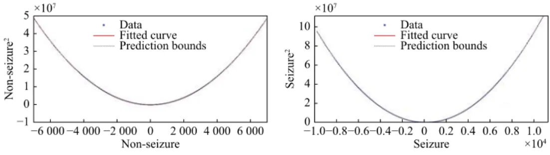
Fig. 1 shows the quadratic linear-parabolic curves obtained for seizure and non-seizure segments, respectively. One notices that the proposed model (7) provides a visually precise fit to the EEG waveform. In addition, the prediction bounds have a small uncertainty throughout the entire data range, hence new observations should be predicted with high accuracy.
Classification
The dataset described above has been used to train the classifier according to the proposed method. The capacity of the proposed classification scheme to discriminate between seizure and non-seizure events in order to detect the seizure onset in EEG signals has been assessed. In Fig. 2, we can observe the great difficulty in discriminating between seizure and non-seizure in EEG raw data. The start and end of the seizure in this EEG signal were labeled by the neurologist using two lines. The first line divides the EEG signal at 81 second (onset) and the second at 162 second (offset).
Table 3 reports the four statistical parameters, calculated for all seizure and non-seizure segments. The weighted sum of squared residuals (ζ) and the root mean squared error (ψ) show much larger values for seizure events with respect to non-seizure events, which suggests that these features can be used to discriminate between seizure and non-seizures in EEG signals. While R-square (ϕ) and adjusted R-square (σ) have values close to one for both types of events, which suggests that the model has high accuracy in the fit. These four parameters show good potential to
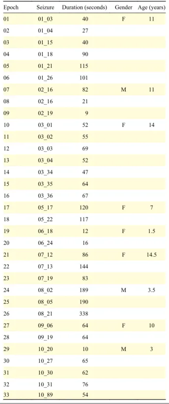
Table 1 Length of the 33 seizures used in this study
Epoch Seizure Duration (seconds) Gender Age (years)
01 01_03 40 F 11 02 01_04 27 03 01_15 40 04 01_18 90 05 01_21 115 06 01_26 101 07 02_16 82 M 11 08 02_16 21 09 02_19 9 10 03_01 52 F 14 11 03_02 55 12 03_03 69 13 03_04 52 14 03_34 47 15 03_35 64 16 03_36 67 17 05_17 120 F 7 18 05_22 117 19 06_18 12 F 1.5 20 06_24 16 21 07_12 86 F 14.5 22 07_13 144 23 07_19 83 24 08_02 189 M 3.5 25 08_05 190 26 08_21 338 27 09_06 64 F 10 28 09_19 64 29 10_20 10 M 3 30 10_27 65 31 10_30 62 32 10_31 76 33 10_89 54
Table 2 The quadratic linear-parabolic model coefficients and the associated 95% confidence bounds (CB)
Coefficients Non-seizure Seizure Value 95% CB Value 95% CB a –0.6855 (–4.095, 2.725) 1.368 (–6.717, 9.453) b 0.9989 (0.9989, 0.9989) 0.9998 (0.9998, 0.9998) c –36.05 (–38.53, –33.57) –35.45 (–41.47, –29.43)
Algorithm 1 Random forest classifier algorithm
D
Data: data set and predictor vector ρ.
Result: ensemble of tree models whose predictions are to be
combined by voting or averaging.
for j=1 to J do
Dj D
1. Take a bootstrap sample of size N from .
Dj
2. Using the bootstrap sample as the training data, fit a tree using binary recursive partitioning:
a. Start with all observations in a single node;
b. Repeat the following steps recursively for each unsplit node until the stopping criterion is met:
i. Select m predictors at random from the ρ available predictors; ii. Find the best binary split among all binary splits on the m predictors from Step i;
iii. Split the node into two descendant nodes using the split from Step ii;
End
discriminate between seizure and non-seizures in EEG signals. This can be visually corroborated in Fig. 1.
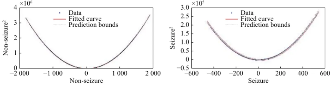
Estimating the four statistical parameters at each 1-second segment allows us to detect changes between epileptic EEG seizures. When we apply equation (7) to each 1-second segments, similar results are obtained as those applied to the signal as a whole. Fig. 3 shows the similarity with Fig. 1. Both seizure and non-seizure events have an excellent fitting with the linear-parabolic model, suggesting that the scale changes and the different values of the estimated parameters can be used to differentiate seizure and non-seizure events in EEG signals.
To cope with the high variability of EEG signals, the features were normalized to be in the range [0,1][33]. Table 4 reports the mean values for the four
statistical parameters ρ=[ζ, ϕ, σ, ψ] calculated for each 1-second segment from X[n]. The weighted sum of squared residuals (ζ) has values closer to zero while R-square (ϕ) and adjusted R-square (σ) have values closer to one. This shows that the model has a high fit accuracy and can be used for seizure detection, as
corroborated by Fig. 3.
A value closer to zero in the weighted sum of squared residuals (ζ) and Root mean squared error (ψ) and values closer to one in R-square (ϕ) and adjusted R-squared (σ) suggest a good fit quality and therefore can be used as a predictor.
Fig. 4 shows the main scatter plots of couples of the normalized statistical parameters (ζ, ϕ, σ, ψ). It is interesting to note that in ζ versus ϕ (Fig. 4A) and ψ versus ϕ (Fig. 4C) the seizure events (red dots) are concentrated closer to one with respect to non-seizure events (blue dots). In Fig. 4B, ζ versus ψ has a big tendency to go to the right in the seizure events (red dots) with respect to non-seizure events (blue dots). In Fig. 4D, ϕ versus σ shows a clear concentration of seizure events (red dots) with respect to non-seizure events (blue dots) on the upper right side. These scatter plots show that our predictor vector ρ=[ζ, ϕ, σ, ψ] is potentially useful to discriminate between seizures and non-seizures events in EEG signals.
To assess the performance of the proposed method, we adopted a supervised testing approach and used 1 518 events (1-second signals) to train and test the method with the 20-fold cross-validation technique of the predictor vector ρ=[ζ, ϕ, σ, ψ]. As explained above, the events were extracted from 33 seizure epochs and 33 non-seizure epochs, giving a total of 66 epochs from 9 different subjects. The method gives good classification performance, with 92% true positives rate (TPR) or sensitivity, 96% true negative rate (TNR) or specificity, 4% false positive rate, and 94.1% accuracy. Please note that segments for training and testing are drawn randomly without consideration of their epochs. This process was repeated 1 000 times to ensure not-bias in the partitioning.
Discussion
This work presented a new method to detect epileptic seizures in EEG signals. The proposed model-based classification method relies on the design Table 3 Goodness-of-fit statistics
Events ζ ϕ σ ψ
Non-seizure 3.624e+14 0.9996 0.9996 4839 Seizure 2.03e+15 0.9999 0.9999 1.145e+04
5 4 3 2 1 0 −1 Non-seizure 2 ×10⁷ −6 000 −4 000 −2 000 0 2 000 4 000 6 000 Non-seizure Data Fitted curve Prediction bounds 10 8 6 4 2 0 Seizure 2 ×107 ×104 −0.8 −1.0 −0.6−0.4−0.2 0 0.2 0.4 0.6 0.8 1.0 Seizure Data Fitted curve Prediction bounds ˜ X X˜2
Fig. 1 Curves of the quadratic linear-parabolic model for seizure and non-seizure events. Note that the scale of the seizure curve
(Right) is much larger than the one of the non-seizure curve (Left). The X-axis represents while the Y-axis represents (the unit on the X and Y axes correspond to the amplitude of the signal). The prediction bounds have a small uncertainty throughout the entire data range, therefore new observations can be predicted with high accuracy.
Amplitude
0 50 100 150 200
Time (seconds)
Fig. 2 EEG raw example. The onset detection begins in 81
seconds according to the medical annotation but by non-expert visual inspection cannot reach the same conclusion. The y-axis scale for each channel is between ±200 mv.
of a specific filter using the two-point central difference algorithm. A linear-parabolic model is fitted to the filtered signal using mean squares. Four statistical parameters associated with the model fitting are used as classification features to discriminate seizure and non-seizure events. A random forest classifier has been adopted to evaluate the ability of these parameters to detect seizures. The proposed methodology was applied to 66 balanced events from the Children Hospital Boston database. Results suggest that the proposed algorithm is a powerful tool for detecting epileptic seizure events in EEG signals achieving a 94.1% accuracy.
The proposed method has two main advantages
compared to existing methods. First, its low computational complexity makes it implementable in quasi-real-time. Second, the method can be easily extended to work separately with different brain rhythms, by adapting the skip factor L. Despite these advantages, the method suffers some limitations, mainly noise and robustness.
The signal is affected by noise and artifacts due to the acquisition and pre-processing. This affects the precision of the results, especially when the method is generalized to complex epileptic forms. Outliers are not directly considered in the estimation procedure that needs more robustness.
Future work will focus on robust approaches to consider noise and artifacts. Optimization techniques will be investigated to remove outliers and improve the accuracy of the detection.
Acknowledgments
Part of the work was conducted by AQR during his Ph.D. work at Buenos Aires Institute of Technology (ITBA).
Table 4 Means of the statistical parameters with values normalized between 0 and 1 for all each 1-second time segments Events ζ ϕ σ ψ Non-seizure 0.14 0.99 0.99 0.30 Seizure 0.11 1.00 1.00 0.25 4 3 2 1 0 Non-seizure 2 ×10⁶ −2 000 −1 000 0 1 000 2 000 Non-seizure Data Fitted curve Prediction bounds −0.5 3.0 2.5 2.0 1.5 1.0 0.5 0 Seizure 2 ×10⁵ −600 −400 −200 0 200 400 600 Seizure Data Fitted curve Prediction bounds ˜ X [n] Fig. 3 Quadratic parabolic curve fitting example for one segment .
1.00 0.98 0.96 0.94 0.92 0.90 0.88 ϕ 0 0.1 0.2 0.3 0.4 0.5 0.6 0.7 0.8 0.9 1.0 0 1 1.0 0.8 0.6 0.4 0.2 0 ψ 0 0.1 0.2 0.3 0.4 0.5 0.6 0.7 0.8 0.9 1.0 ζ ζ 0 1 1.00 0.98 0.96 0.94 0.92 0.90 0.88 ϕ 0 0.1 0.2 0.3 0.4 0.5 0.6 0.7 0.8 0.9 1.0 0 1 1.00 0.98 0.96 0.94 0.92 0.90 0.88 σ 0.88 0.90 0.92 0.94 0.96 0.98 1.00 ϕ ψ 0 1 ζ vs. ϕ ζ vs. ψ ψ vs. ϕ ϕ vs. σ A B C D
Fig. 4 Scatter plots for the four statistical parameters (ζ, ϕ, σ, ψ) observed through 1 518 events from 66 epochs, 33 seizures (red dots) and 33 on-seizures (blue dots) before the seizure. The weighted sum of squared residuals (ζ), R-square (ϕ), adjusted R-squared (σ)
References
Frei MG, Davidchack RL, Osorio I. Least squares acceleration filtering for the estimation of signal derivatives and sharpness at extrema [and application to biological signals][J]. IEEE
Trans Biomed Eng, 1999, 46(8): 971–977.
[1]
Chernov N, Lesort C. Statistical efficiency of curve fitting algorithms[J]. Comput Stat Data Anal, 2004, 47(4): 713–728. [2]
López-Rubio E, Thurnhofer-Hemsi K, Blázquez-Parra EB, et al. A fast robust geometric fitting method for parabolic curves[J]. Pattern Recognit, 2018, 84: 301–316.
[3]
Zhang HH, Su JZ, Wang QY, et al. Predicting seizure by modeling synaptic plasticity based on EEG signals - a case study of inherited epilepsy[J]. Commun Nonlinear Sci Numer
Simul, 2018, 56: 330–343.
[4]
Ramon C, Holmes MD, Wise MV, et al. Oscillatory patterns of phase cone formations near to epileptic spikes derived from 256-channel scalp EEG data[J]. Comput Mathem Methods
Med, 2018, 2018: 9034543.
[5]
Liu HY, Yang Z, Meng FG, et al. Chronic vagus nerve stimulation reverses heart rhythm complexity in patients with drug-resistant epilepsy: an assessment with multiscale entropy analysis[J]. Epilepsy Behav, 2018, 83: 168–174.
[6]
Begemann A, Acuña MA, Zweier M, et al. Further corroboration of distinct functional features in SCN2A variants causing intellectual disability or epileptic phenotypes[J]. Mol
Med, 2019, 25: 6.
[7]
Liang SF, Wang HC, Chang WL. Combination of EEG complexity and spectral analysis for epilepsy diagnosis and seizure detection[J]. EURASIP J Adv Sign Processing, 2010, 2010: 853434.
[8]
Sorensen TL, Olsen UL, Conradsen I, et al. Automatic epileptic seizure onset detection using matching pursuit: a case study[C]//Proceedings of 2010 Annual International Conference of the IEEE Engineering in Medicine and Biology. Buenos Aires, Argentina: IEEE, 2010: 3277-3280.
[9]
Nasehi S, Pourghassem H. A novel fast epileptic seizure onset detection algorithm using general tensor discriminant analysis[J]. J Clin Neurophysiol, 2013, 30(4): 362–370. [10]
Zhang ZN, Wen TX, Huang W, et al. Automatic epileptic seizure detection in EEGs using MF-DFA, SVM based on cloud computing[J]. J X-Ray Sci Technol, 2017, 25(2): 261–272.
[11]
Mahmoodian N, Boese A, Friebe M, et al. Epileptic seizure detection using cross-bispectrum of electroencephalogram signal[J]. Seizure, 2019, 66: 4–11.
[12]
Polychronaki G, Ktonas P, Gatzonis S, et al. Comparison of fractal dimension estimation algorithms for epileptic seizure onset detection[J]. J Neural Eng, 2014, 7(4): 046007.
[13]
Birjandtalab J, Pouyan MB, Cogan D, et al. Automated seizure detection using limited-channel EEG and non-linear dimension reduction[J]. Comput Biol Med, 2017, 82: 49–58.
[14]
Acharya UR, Oh SL, Hagiwara Y, et al. Deep convolutional neural network for the automated detection and diagnosis of seizure using EEG signals[J]. Comp Biol Med, 2018, 100: [15]
270–278.
Quintero-Rincón A, Pereyra M, D'Giano C, et al. Fast statistical model-based classification of epileptic EEG signals[J]. Biocybern Biomed Eng, 2018, 38(4): 877–889. [16]
Breiman L. Random forests[J]. Mach Learn, 2001, 45(1): 5–32. [17]
Flach P. Machine learning[M]. Cambridge: Cambridge University Press, 2012.
[18]
Manzouri F, Heller S, Dümpelmann M, et al. A comparison of machine learning classifiers for energy-efficient implementation of seizure detection[J]. Front Syst Neurosci,
2018, 12: 43. [19]
Le Douget JE, Fouad A, Maskani Filali M, et al. Surface and intracranial EEG spike detection based on discrete wavelet decomposition and random forest classification[C]// Proceedings of the 39th Annual International Conference of the IEEE Engineering in Medicine and Biology Society. Seogwipo, South Korea: IEEE, 2017: 475-478.
[20]
Donos C, Dümpelmann M, Schulze-Bonhage A. Early seizure detection algorithm based on intracranial EEG and random forest classification[J]. Int J Neural Syst, 2015, 25(5): 1550023. [21]
López S, Suarez G, Jungreis D, et al. Automated identification of abnormal adult EEGs[C]//Proceedings of 2015 IEEE Signal Processing in Medicine and Biology Symposium. Philadelphia, PA, USA: IEEE, 2015.
[22]
Shoeb A, Edwards H, Connolly J, et al. Patient-specific seizure onset detection[J]. Epilepsy Behav, 2004, 5(4): 483–498. [23]
Goldberger AL, Amaral LA, Glass L, et al. PhysioBank, PhysioToolkit, and PhysioNet: components of a new research resource for complex physiologic signals[J]. Circulation, 2000, 101(23): E215–E220.
[24]
Sanei S. Adaptive processing of brain signals[M]. United Kingdom: Wiley, 2013.
[25]
Bahill AT, McDonald JD. Frequency limitations and optimal step size for the two-point central difference derivative algorithm with applications to human eye movement data[J].
IEEE Trans Biomed Eng, 1983, 30(3): 191–194.
[26]
Tseng CC, Lee SL. Design of digital differentiator using difference formula and Richardson extrapolation[J]. IET Sign
Process, 2008, 2(2): 177–188.
[27]
Semmlow JL, Griffel B. Biosignal and medical image processing[M]. 3rd ed. Boca Raton: CRC Press, 2014. [28]
Hansen PC, Pereyra V, Scherer G. Least squares data fitting with applications[M]. Baltimore: Johns Hopkins University Press, 2013.
[29]
Neuhauser C. Calculus for biology and medicine[M]. 2nd ed.
Upper Saddle River, NJ: Pearson, 2004. [30]
Samarasinghe G, Sowmya A, Moses DA. A semi-quantitative analysis model with parabolic modelling for DCE-MRI sequences of prostate[C]//Proceedings of 2014 International Conference on Digital Image Computing: Techniques and Applications. Wollongong, NSW, Australia: IEEE, 2014. [31]
Zhang C, Ma YQ. Ensemble machine learning: methods and applications[M]. Boston, MA: Springer, 2012.
[32]
Quintero-Rincón A, Carenzo C, Ems J, et al. Spike-and-wave epileptiform discharge pattern detection based on Kendall's Tau-b coefficient[J]. Appl Med Inform, 2019, 41(1): 1–8. [33]