Evolution of the rainfall regime in the United Arab Emirates
1T.B.M.J. Ouarda1, 2*, C. Charron1, K. Niranjan Kumar1, P. R. Marpu1, H. Ghedira1, A. 2
Molini1 and I. Khayal3 3
4 1
Institute Center for Water and Environment (iWATER), Masdar Institute of Science and 5
Technology, P.O. Box 54224, Abu Dhabi, UAE 6
2
INRS-ETE, National Institute of Scientific Research, Quebec City (QC), G1K9A9, 7
Canada 8
3
Engineering Systems and Management, Masdar Institute of Science and Technology, 9
P.O. Box 54224, Abu Dhabi, UAE 10 11 12 *Corresponding author: 13 Email: [email protected] 14 Tel: +971 2 810 9107 15 16 17
To be submitted to Journal of Hydrology 18
March 2013 19
Abstract
21
Arid and semiarid climates occupy more than 1/4 of the land surface of our planet, and 22
are characterized by a strongly intermittent hydrologic regime, posing a major threat to 23
the development of these regions. Despite this fact, a limited number of studies have 24
focused on the climatic dynamics of precipitation in desert environments, assuming the 25
rainfall input – and their temporal trends – as marginal compared with the evaporative 26
component. Rainfall series at four meteorological stations in the United Arab Emirates 27
(UAE) were analyzed for assessment of trends and detection of change points. The 28
considered variables were total annual, seasonal and monthly rainfall; annual, seasonal 29
and monthly maximum rainfall; and the number of rainy days per year, season and 30
month. For the assessment of the significance of trends, the modified Mann-Kendall test 31
and Theil-Sen’s test were applied. Results show that most annual series present 32
decreasing trends, although not statistically significant at the 5% level. The analysis of 33
monthly time series reveals strong decreasing trends mainly occurring in February and 34
March. Many trends for these months are statistically significant at the 10% level and 35
some trends are significant at the 5% level. These two months account for most of the 36
total annual rainfall in the UAE. To investigate the presence of sudden changes in rainfall 37
time-series, the cumulative sum method and a Bayesian multiple change point detection 38
procedure were applied to annual rainfall series. Results indicate that a change point 39
happened around 1999 at all stations. Analyses were performed to evaluate the evolution 40
of characteristics before and after 1999. Student’s t-test and Levene’s test were applied to 41
determine if a change in the mean and/or in the variance occurred at the change point. 42
Results show that a decreasing shift in the mean has occurred in the total annual rainfall 43
and the number of rainy days at all four stations, and that the variance has decreased for 44
the total annual rainfall at two stations. Frequency analysis was also performed on data 45
before and after the change point. Results show that rainfall quantile values are 46
significantly lower after 1999. The change point around the year 1999 is linked to various 47
global climate indices. It is observed that the change of phase of the Southern Oscillation 48
Index (SOI) has strong impact over the UAE precipitation. A brief discussion is presented 49
on dynamical basis, the teleconnections connecting the SOI and the change in 50
precipitation regime in the UAE around the year 1999. 51
52
Keywords
53
Rainfall; Arid-climate; Trend; Change-point; Extreme; Seasonality, Teleconnection, 54
Southern Oscillation Index. 55
1. Introduction
57
The United Arab Emirates (UAE) is located in the arid southeast part of the Arabian 58
Peninsula. This region is characterized by very scarce and variable rainfall. Without 59
permanent surface water resources, groundwater resources were extensively used for 60
water supply. Recently, strong economic and demographic growth in UAE has put even 61
more stress on water resources. The deficit in water availability between the increasing 62
demand and water resources availability has been met by non-conventional sources such 63
as desalinated water. Groundwater aquifers rely on recharge from rainfall. For this 64
purpose, a large number of small recharge dams were built to capture rainfall water from 65
infrequent but usually intense events. For optimal water resources management, it is 66
important to understand the temporal evolution of rainfall. The main objective of the 67
present study is to analyze rainfall trends in the arid region of the UAE. The variables 68
analyzed in this study are: the total annual, seasonal and monthly rainfall; the annual, 69
seasonal and monthly maximum rainfall, and the number of rainy days per year, season 70
and month. 71
A relatively limited number of studies dealing with rainfall trend analysis in arid and 72
semi-arid regions have been conducted, with very few dealing with desert environments 73
and the Arabian Peninsula. Modarres and Sarhadi (2009) found that, in Iran, annual 74
rainfall is decreasing at 67% of 145 stations studied while annual maximum rainfall is 75
decreasing at only 50% of the stations. However, only 24 stations exhibit significantly 76
negative trends. Törnros (2010) reported a statistically significant decreasing trend at 5 77
stations among a total of 37 stations in the southeastern Mediterranean region. 78
Decreasing but non-significant trends in rainfall characteristics were found in the region 79
of Oman by Kwarteng et al. (2009). Gong et al. (2004) observed slightly decreasing 80
trends in rainfall amounts in the semi-arid region of northern China. However, other 81
rainfall characteristics, such as number of rainy days, maximum daily rainfall, 82
precipitation intensity, persistence of daily precipitation and dry spell duration, 83
experienced significant changes. 84
Hess et al. (1995) found significant decreasing trends in annual rainfalls and in the 85
number of rainy days per year in the arid Northeast part of Nigeria. Neither trends nor 86
abrupt changes in rainfall characteristics were found by Lazaro et al. (2001) at a station 87
located in the semi-arid southeastern part of Spain. Batisani and Yarnal (2010) found 88
significant decreasing trends for rainfall amounts, associated with a decrease in the 89
number of rainy days throughout semi-arid Botswana. In general, most studies conducted 90
in arid or semi-arid regions found decreasing trends in the rainfall regime of these areas. 91
Output of global and regional climate models indicate also an anticipated decrease in 92
rainfall amounts in most arid and semi-arid regions of the globe, although predicted 93
scenarios for arid areas present a high degree of variability (Black et al., 2010; 94
Chenoweth et al., 2011; Hemming et al., 2010). 95
In this study, a modified version of the original Mann-Kendall (MK) test, to account for 96
serial correlation, was used for the assessment of trends in rainfall time series. The MK 97
test is one of the most commonly used statistical tests for trend detection in hydrological 98
and climatological time series (Türkeş, 1996; Gan, 1998; Fu et al., 2004; Lana et al., 99
2004; Khaliq et al., 2008, 2009a, 2009b; Modarres and Sarhadi, 2009; Fiala et al., 2010). 100
The main advantage of using a non-parametric statistical test is that it is more suitable for 101
meteorological time series (Yue et al., 2002a). The presence of sudden changes in rainfall 103
time series was also investigated. For this, two methods were used. The first one is the 104
cumulative sums method (Cusum). It is a simple graphical method that allows detecting 105
changes in the mean by identification of linear trends in the plot of the cumulative values 106
of deviations. The second one is a Bayesian multiple change point detection procedure. It 107
can be used to detect changes in the relation of the response variable with explanatory 108
variables. When time is used as explanatory variable, the procedure allows detecting 109
temporal changes in the time-series. Changes in the mean and the variance are also 110
investigated in this study. An analysis and a discussion of the physical causes of any 111
observed changes are also presented in the present work. 112
The present paper is organized as follows: Section 2 presents the data used in this study. 113
In section 3, the methods used are summarized. Results are presented and discussed in 114
section 4, and conclusions are presented in section 5. 115
116
2. Data
117
The UAE is located in the Southeastern part of the Arabian Peninsula. It is bordered by 118
the Gulf in the north, Oman in the east and Saudi Arabia in the south. It lies 119
approximately between 22°40’N and 26°N and between 51°E and 56°E. The total area of 120
the UAE is about 83600 km2 and 90% of the land is classified as hot desert. The rest is 121
mainly represented by the mountainous region in the Northeastern part of the country. 122
The climate of the UAE is arid. Rainfall is scarce and shows a high temporal and spatial 123
variability. The mean annual rainfall in the UAE is about 78 mm and ranges from 40 mm 124
in the southern desert region to 160 mm in the northeastern mountains (FAO, 1997). 125
The data used in this study comes from 4 meteorological stations located in the 126
international airports of the UAE. Total rainfall is recorded on a daily basis. The map in 127
Fig. 1 gives the spatial distribution of the meteorological stations and shows that the 128
western region of the country is not represented in the database. Periods of record range 129
from 30 to 37 years. The station of Ras Al Khaimah is located near the northeastern 130
mountainous region while the Abu Dhabi, Dubai and Sharjah stations are located along 131
the northern coastline. 132
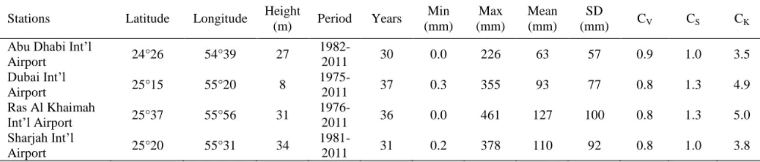
A list of the rainfall stations as well as basic statistics of the annual rainfall data are given 133
in Table 1. This includes minimum, maximum, mean, standard deviation, coefficient of 134
variation, coefficient of skewness and coefficient of kurtosis. In average, Abu Dhabi 135
receives the smallest amount of rain (63 mm) and Ras Al Khaimah receives the highest 136
amount (127 mm). Minimum total annual rainfall amounts are very low for all stations. 137
The variability of annual rainfall time series is high for all stations with values of the 138
coefficient of variation around one. All skewness values are positive indicating right 139
skewed distributions. 140
From the daily data, the following variables are computed: total annual and monthly 141
rainfall, annual and monthly maximum daily rainfall, and number of rainy days per year 142
and per month. The number of rainy days is defined here by the number of days per year 143
or per month with an amount of water higher than 0.1 mm. In the present study, the 144
hydrological year starting on September 1st and ending on August 31th has been 145
considered for the computation of annual rainfall series. September 1st has been selected 146
to start the hydrological year because this date is located during a particularly dry period. 147
The use of the calendar year (January 1st to December 31st) would have resulted in 148
splitting the rainy season between two years. Monthly mean values for each variable are 149
presented in Fig. 2. This figure indicates that the majority of the rain falls between 150
December and March for all stations. The figure shows also that the peak of the rainy 151
season occurs earlier (December) in the eastern region and later as we go towards the 152
central region of the UAE. Fig. 3 illustrates the seasonality of rainfall in the UAE through 153
the polar plots of mean monthly maximum rainfalls in the four stations. 154 155
3. Methods
1563.1. Mann-Kendall test
157The non-parametric test of MK (Mann, 1945; Kendall, 1975) was applied to time-series 158
for assessment of trends. For a given data sample x x1, 2,...,xn of size n, the MK test 159
statistic S is defined by: 160 1 1 1 sgn( ) n n j i i j i S x x
( 1 ) 161where x and i xjare the data values for periods i and j respectively and the sgn(xj - xi) is
162
the sign function given by: 163
1 if - 0 sgn( ) 0 if - 0 1 if - 0 j i j i j i j i x x x x x x x x ( 2 ) 164
For large values of n, the distribution of the S statistic can be well approximated by a 165
normal distribution, with mean and variance given respectively by: 166 E( )S 0 ( 3 ) 167 1 ( 1)(2 5) ( )( 1)(2 5) Var( ) 18 m i i n n n t i i i S
( 4 ) 168where m is the number of tied values and ti is the number of ties for the ith tied value. The
169
standardized normal test statistic Zs is given by:
170 1 if S > 0 Var( ) 0 if S = 0 1 if S < 0 Var( ) S S S Z S S ( 5 ) 171
A positive value of Zs indicates an increasing trend while a negative value of Zs indicates
172
a decreasing trend. The null hypothesis can be rejected at a significance level of p if Zs
173
is greater that Z1p/2 where Z1p/2 can be obtained from the standard normal cumulative
174
distribution tables. 175
To limit the influence of the serial correlation, Hamed and Rao (1998) proposed to 176
modify the variance of the MK statistic S to account for autocoerrelation in the data. In 177
this paper, the variance is corrected by considering the lag-1 autocorrelation. The 178
correction of the variance is applied to Zs only when the sample lag-1 serial correlation
coefficient is significant. In this study, the linear trend is removed from the series before 180
computing the effective sample size. 181
3.2. Cumulative sum method
182
The cumulative sum (Cusum) method is a graphical approach that is often used for the 183
detection of changes in time series. For a given time series x x1, 2,...,x , the cumulative n
184
sum of deviations for any time k is given by: 185 1 ( )
k k i i S x x ( 6 ) 186Cusum values, given by Sk, are graphically represented as a function of k. Substantial
187
negative or positive slopes indicate sequences of values below or above the mean value. 188
The positions at the intersection of change of slope indicate change points. 189
3.3. Bayesian multiple change point detection procedure
190
To detect changes in rainfall time series, the Bayesian multiple change point detection 191
procedure (Seidou and Ouarda, 2007) is used. This technique represents a general 192
procedure to detect the number, magnitudes and positions of multiple change points in 193
the relationship between a set of explanatory variables and a response variable. If no 194
explanatory variables are specified, the procedure detects changes in the time series of the 195
response variable. The response variable is denoted yj(j1,..., )n or ynx1 in vectorial 196
form, while x iij( 1,..., ;d j1,..., )n represents the j
th
observation of the ith explanatory 197
variable (Xd*xn in matrix form). There are n observations and d* explanatory variables.
198
The multiple linear relationship can be represented as: 199
* 1 , 1,..., d j i ij j i y x j n
( 7 ) 200More details about this procedure and the inference of the number and positions of 201
change points are given in Seidou and Ouarda (2007). In this study, we are interested in 202
detecting chronological changes in the time series. 203
3.4. Frequency analysis
204
In the present study, fitting of the data is performed in the Matlab environment. For each 205
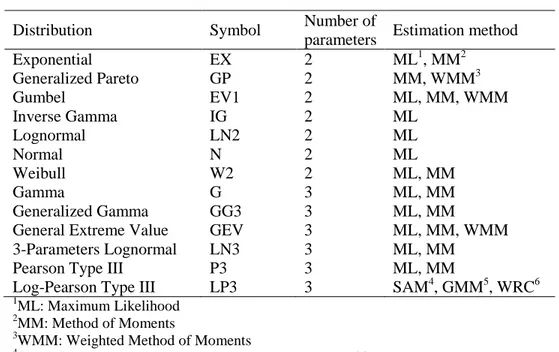
statistical distribution, a number of efficient fitting methods are considered. A list of 206
“distributions/estimation methods” selected for fitting the data series is presented in 207
Table 2. To evaluate the goodness of fit of the different distributions/methods, the Akaïke 208
information criterion (AIC) (Akaïke, 1970) is used. The model leading to the minimum 209
value of the AIC is the model with the best fit. The AIC is a parsimonious criterion as it 210
takes into consideration the number of estimated parameters in the model following the 211
law of parsimony. 212
3.5. Student’s t-test for equality of means
213
The Student’s t-test is used to test the null hypothesis H0 that the means from two 214
samples are equal against the alternative hypothesis H1 that the means are different. Let 215
1j( 1,..., )1
x j n and x2j(j1,...,n2) be two samples of length n and 1 n with means 2 x 1
216
and x and variances 2 2 1
s and s22. The Student’s test statistic is computed as :
1 2 2 2 1 2 1 2 x x t s s n n ( 8 ) 218
The null hypothesis can be rejected at a significance level of p if t t1p/2, where t1p/ 2,
219
can be obtained from a t-table with degrees of freedom. 220
3.6. Levene’s test for equality of variances
221
The Levene’s test (Levene, 1960) is used to test the equality of variances of k samples. 222
For data samples x1j(j1,..., )n1 and x2j(j1,...,n2) , we define z1j x1jx1 and 223
2j 2j 2
z x x where x and 1 x are the medians of the first and the second sample 2
224
respectively. The Levene’s test statistic is defined as: 225 1 2 2 2 1 2 1 1 12 2 2 12 2 2 1 1 2 2 1 1 ( 2)[ ( ) ( ) ] ( ) ( ) n n j j j j n n n Z Z n Z Z W Z Z Z Z
( 9 ) 226 where 1 1 1 1 1 1 n j j Z z n
, 2 2 2 1 2 1 n j j Z z n
and 1 2 12 1 2 1 1 1 2 1 n n j j j j Z z z n n
. The null 227hypothesis, that the variances of the two samples are equal, can be rejected at a 228 significance level of p if 1 2 1 p/2,1,n n 2 W F . 229
3.7. Theil-Sen’s slope estimator
230
The true magnitude of a slope of a given data sample x x1, 2,...,x , can be estimated with n
231
the Theil-Sen’s estimator (Theil, 1950; Sen, 1968), which is given by: 232 median xj xi 1 b i j j i ( 10 ) 233
where x and i xj are the ith and jth observations. It is a robust estimate of the slope of 234
the trend (Yue et al., 2002b). This method has been recently used to obtain the magnitude 235
of trends in evapotranspiration by Dinpashoh et al. (2011), in temperature by Jhajharia et 236
al. (2013) and in groundwater level and quality by Daneshvar Vousoughi et al. (2013). 237
238
4. Results and discussion
239
Annual time series of all variables for selected stations are presented in Fig. 4. The dotted 240
line represents the linear trend in each series. In the following, only the results given by 241
the modified Mann-Kendall test are presented and commented as they are more reliable 242
in the presence of serial correlation. However, the differences between the results of the 243
classical MK test and the modified MK test are minor. Table 3 presents the results of the 244
modified MK test. It shows the Z statistics obtained at each station for each rainfall 245
variable. Statistically significant trends at levels 5% and 10% are identified with the 246
indices a and b respectively over the corresponding Z values. 247
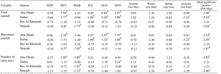
The Z statistics indicate that the majority of annual series have decreasing trends. 248
However, none of these trends are statistically significant. Analysis of the monthly trends 249
reveals that the strongest trends occur during February and March. During these months, 250
all trends are decreasing. Some of the trends are significant at the level of 5% and several 251
are significant at the level of 10%. These trends are important because these two months 252
contribute for most of the total annual rainfall. Several other significant trends occur 253
during July and August for monthly rainfall and maximum rainfalls. Most of the trends 254
are also decreasing during these two months. Some significantly positive trends are also 255
recorded during the month of November. 256
To further investigate seasonal trends, months have been grouped together into 4 seasons. 257
In addition, the months with the most significant Z statistics, February and March, were 258
grouped together. Again, only the results of the modified Mann-Kendall test are 259
presented and discussed. However, the classical and the modified versions of the MK test 260
led to similar results. Table 3 presents the results of the modified MK test. Winter and 261
summer show decreasing trends, spring shows slightly decreasing trends and autumn 262
shows mixed decreasing and increasing trends. However, not all trends are significant. 263
For Dubai, the total rainfall and the maximum rainfall have a significant decreasing trend 264
at 5% and for Sharjah, the number of rainy days has a significant decreasing trend at a 265
level of 10%. When February and March are grouped together, all trends are decreasing 266
and several trends are significant at the level of 5% and 10%. 267
Cusum plots are used to investigate the presence of change points in the mean of the time 268
series. For every time series, a change of slope occurs in 1999. Before 1999, slopes are 269
positive and afterwards they become negative until the end of the series. 270
The Bayesian multiple change point detection procedure was also applied to each annual 271
series as well as the series of the dates of maximum annual rainfall. Fig. 5 illustrates the 272
identified change points and presents the trends for the various segments for the number 273
of rainy days by year series. The results for the other variables lead to identical patterns 274
for all 4 stations and are not presented due to space constraints. It is relevant to mention 275
that the results presented in Fig 5 are for segments with at least 6 years of data, in order to 276
avoid identifying change points that are too close to the edges of the series or for which 277
not enough data is available to justify the conclusions. The Bayesian procedure was also 278
carried out for segments with at least 3, 4 or 5 years of data, and the results were 279
consistent with the ones obtained with segments of 6 years of data. 280
For most of the series, a shift is detected in 1999 or around this year. Note that given the 281
random nature of the natural variables being analyzed, the exact date of change may not 282
be as important as the existence of the change, the approximate year and the general 283
trends before and after the change. The exact date may be one or two years different from 284
the detected one, depending on the random component for the years neighboring the 285
change. The detected shift confirms the results obtained with the Cusum method. In 286
general, no change in the date of the maximum rainfall is detected. The results of the 287
Bayesian multiple changepoint detection procedure allow for refining our knowledge 288
concerning the evolution of the rainfall regime in the UAE. While the modified MK test 289
results point to a decreasing trend in all variables associated to the rainfall regime, the 290
change point procedure allows us to see that the general trends in these variables are in 291
fact positive throughout the period of record, but with a downward jump around 1999. 292
Based on these results, it was decided to separate the annual series into two subsamples at 293
the change point year of 1999. The first subsample includes the data from the beginning 294
of each series to 1998 and the second one includes the data from 1999 to the end of each 295
series. The significance of the change in the mean and in the variance in each pair of 296
subsamples is evaluated with the Student’s t-test and the Levene’s test. Results show that 297
there is a shift in the mean of the total annual rainfall and in the mean of the number of 298
rainy days for the four stations. The Levene’s test results indicate also a change in the 299
variance of the total annual rainfall for the stations of Abu Dhabi and Dubai. 300
Fig. 6 presents bar diagrams of the monthly mean values for the total annual rainfall 301
before and after the change in 1999. These diagrams show that, for the months of 302
January, February, March, April and July, most of the stations experienced an important 303
drop in rainfall. The most important drops happened during the months of February and 304
March. For December, rainfall remained about constant for most of the stations. For the 305
other months, rainfall amounts are very low and conclusions cannot be drawn. 306
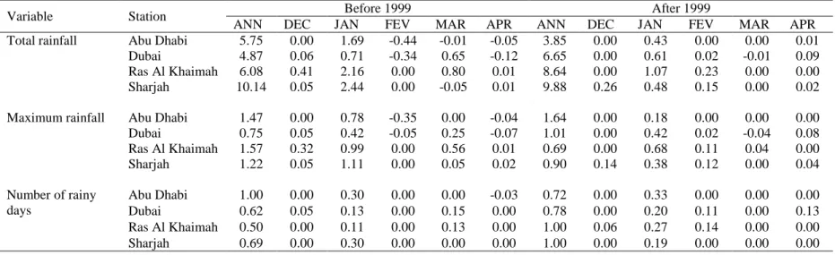
True slopes in rainfall variables were investigated with the Theil-Sen’s estimator. Table 4 307
gives the slopes for annual rainfall series and monthly rainfall series for months with 308
significant amount of rainfall before and after the change in 1999. Increasing trends for 309
annual rainfalls, when the samples are divided at the change point, are confirmed with 310
positive slopes for all annual rainfall series. 311
Fig. 7 presents, in a single polar plot, the annual maximum rainfall for all stations. The 312
blue stars represent the values before the change of 1999 and the red circles indicate the 313
values after the change. Fig. 7 indicates a general decrease in the magnitudes of the 314
maxima for the second portion of the series (after the 1999 change). A shift in the months 315
in which the maxima occurred can also be observed. Indeed, for the first portion of the 316
series, the annual maxima happened generally during the months of February and March, 317
while they happened usually between December and February for the second portion. 318
Fig. 7 confirms that the overall decrease in annual maximum rainfalls observed in all 319
stations after 1999 is also associated to a shift in the timing of these maxima. In general, 320
annual maximum rainfalls seem to be occurring earlier in the winter season during the 321
second segment of the series. 322
A frequency analysis was also performed on the subsamples of each annual time series 323
for all four stations. All the Distributions/Methods presented in Table 2 were fitted to 324
each subsample (before and after 1999) and, based on the Akaïke criterion, the best 325
Distributions/Methods are selected for each one. Results are presented in Table 5 for the 326
annual total rainfalls, annual maximum rainfalls and number of rainy days. Quantiles 327
corresponding to a number of return periods are presented for each subsample. It can be 328
observed that, for most stations and variables, the values of quantiles drop significantly 329
after the change point. Results presented also include the return periods corresponding to 330
the second subsamples. To compute these return periods, the probabilities corresponding 331
to the quantiles obtained from the first subsample of a given rainfall series are obtained 332
from the distribution and parameters fitted on the second subsample. 333
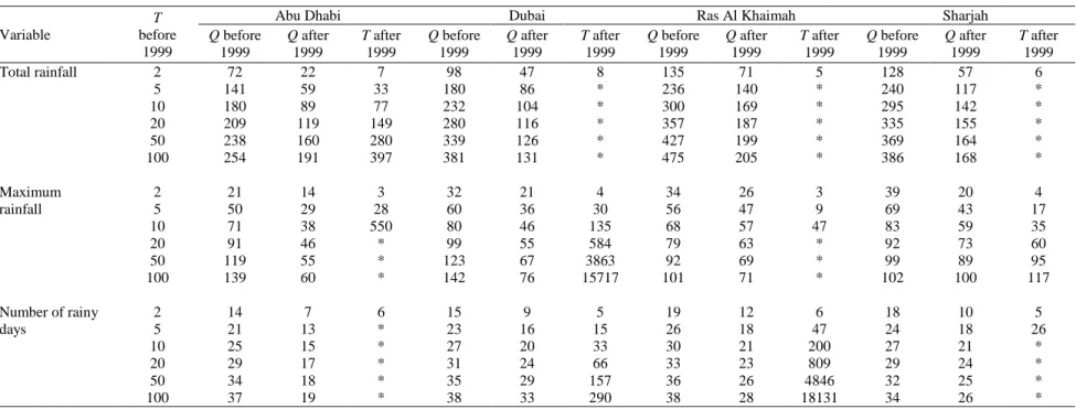
For instance, at the Abu Dhabi station, and for annual maximum rainfalls, the value of the 334
quantile corresponding to the T =10 year return period before 1999 is 71 mm. This same 335
value (71 mm) corresponds to a return period of T = 550 years for the second subsample 336
(after 1999). This drastic increase in the return period corresponding to this annual 337
maximum rainfall value clearly illustrates the differences in the rainfall regimes at the 338
Abu Dhabi station before and after 1999. 339
For the Dubai, Ras Al Khaimah, and Sharjah stations, the return periods corresponding to 340
the 10-year annual maximum rainfall quantile for the first subsample of the series (before 341
1999) correspond respectively to 135 years, 47 years and 35 years for the second 342
subsample. The differences of the rainfall regimes before and after 1999 at these four 343
stations are so large that a number of return periods cannot be calculated because, often 344
the value of a quantile from the first subsample falls beyond the upper limit of the 345
distribution fitted on the second subsample. This is true for annual total rainfalls, annual 346
maximum rainfalls and number of rainy days per year (Table 5). 347
However, it is important to put a word of caution. The use of the results presented above 348
has to be done prudently: While it is important to identify trends and jumps in hydro-349
climatic series, the direct extrapolation of the currently observed trends can be misleading 350
and can convey erroneous results. It is not recommended to extrapolate these results 351
linearly into the future or to extrapolate them for the estimation of quantiles 352
corresponding to large return periods, given the short record length (see Ouarda and El 353
Adlouni, 2011). It is important to carry out the effort of analyzing and understanding the 354
physical mechanisms associated to the inter-annual variability in the rainfall series in the 355
Gulf region. 356
The analysis of the possible connections between climate oscillation signals and 357
precipitation variability in the UAE is an important step. A number of low frequency 358
climate oscillation indices have been shown to play a role in the success or failure of 359
Indian Monsoon development and to impact hydro-climatic variables in the Indian Ocean 360
region. These include for instance the Southern Oscillation Index (SOI), the Pacific 361
Decadal Oscillation (PDO), the El Niño-Southern Oscillation (ENSO), the East Atlantic 362
(EAO), the Atlantic Multidecadal (AMO), and the Indian Ocean Dipole (IOD) indices 363
(Rasmusson and Carpenter, 1983; Kripalani and Kulkarni, 1997; Kumar et al., 1999, 364
2006; Krishnamurthy and Goswami, 2000; Ashok et al., 2001; Sahai et al., 2003; 365
Kripalani et al., 2003; Selvaraju, 2003; Krishnan and Sugi, 2003; Maity and Kumar, 366
2006; NOAA, 2006). 367
Fig. 8 illustrates cumulative values of a number of climate indices of potential interest for 368
the Gulf region. The figure indicates that the year 1999 (or somewhere around it) 369
corresponds to a change of phase of these indices. This could explain the shift that was 370
observed in all precipitation variables and in all UAE stations around this year. 371
Correlation values between these low frequency oscillation climate indices and rainfall 372
variables at the six stations of the study are high and reach the value of 0.68. 373
Nazemosadat et al. (2006) carried out an analysis to detect change-points in precipitation 374
time series in Iran during the 1951-1999 period. They observed a change point in 375
precipitation around 1975 associated with a positive trend during the period after 1975. A 376
strong relationship of precipitation with ENSO events was detected. Nazemosadat et al. 377
(2006) emphasized that precipitation in southern Iran is higher during El Nino periods 378
and weaker during La Nina. Several other authors identified relationships between 379
precipitation and climate oscillation patterns in the Middle East and the ENSO and NAO 380
indices. ENSO was stated to have an influence on climate in southwest Iran (Dezfuli et 381
al., 2010) and Turkey (Karabörk and Kahya, 2003; Karabörk et al., 2005), while NAO 382
was stated to have an influence on meteorological droughts in southwest Iran (Dezfuli et 383
al., 2010), on precipitation and streamflow patterns in Turkey (Kahya, 2011) and on the 384
Middle Eastern climate and streamflow in general (Cullen et al., 2002). The change in 385
precipitation regime in the UAE that is recorded in the present study after 1999 and the 386
fact that this year corresponds also to a change in the SOI phase confirm that ENSO has a 387
the non-linearity and nonstationarity of the SOI volatility have increased in recent 389
decades and that ENSO has become more dynamic and uncertain. This may increase the 390
prediction uncertainty of ENSO-driven climate phenomena. 391
As cited above, there are several statistical connections between ENSO events and 392
precipitation anomalies around the world. However, it is important to understand how the 393
Sea Surface Temperature (SST) anomalies characteristic of ENSO warm phase (El Niño) 394
and cold phase (La Niña) change the weather patterns over the UAE and the Arabian 395
Peninsula's precipitation. Here, we present a discussion of the teleconnection mechanism 396
that controls the precipitation over the UAE and adjacent regions. 397
During the ENSO warm phase the air rising at upper levels of the atmosphere eventually 398
diverges. The anomalous divergence and associated vorticity changes in the upper 399
troposphere drive the atmospheric Rossby waves that affect the global atmospheric 400
circulations. The jet streams in the upper troposphere act as wave-guides for the planetary 401
Rossby waves. The anomalous warming in central and eastern Pacific during the ENSO 402
events (warm and cold phase) alters the position of the troughs and ridges of the Rossby 403
waves (e.g., Straus and Shukla, 1997). As an example, we plotted in Figs. 9a & b, the 404
anomalous meridional wind derived from the National Center for Environmental 405
Prediction- Department of Energy (NCEP-DOE) Reanalysis-2 data (Kanamitsu et al., 406
2002) at 300hPa pressure level (v300hPa) during the winter period (DJFM) of 1997/98 407
and 2005/06 respectively. The two years happen to coincide with the ENSO warm and 408
cold phase respectively. One can observe the alternating positive and negative v300hPa 409
anomalies in the upper troposphere associated with Rossby waves. 410
It is also evident from Fig. 9 that there is distinct change of phase of the upper 411
tropospheric Rossby waves during these anomalous winter periods. These large-scale 412
atmospheric teleconnection patterns alter the surface energy balance in extra-tropics, 413
largely due to surface wind speed anomalies affecting sensible and latent heat fluxes 414
(Deser and Blackmon, 1995). This "atmospheric bridge" is expected to operate most 415
effectively during winter when the strong westerly jet streams persistent in the upper 416
troposphere are favorable for the propagation of Rossby waves. 417
The teleconnection mechanism discussed above shows that ENSO has a strong impact on 418
the UAE precipitation. As discussed previously there exists a change point in the 419
precipitation regime over the UAE around the year 1999. This change should also be 420
reflected in the upper tropospheric flows. In order to see this change point, we have 421
applied the Principal Component Analysis (PCA) to v300hPa anomalies (0oN-60oN) 422
during the winter for the period, 1979-2012. Figs. 10a & b show the time series and 423
spatial pattern of the first principal component (PC1). It is evident from Fig. 10a that 424
there exists inter-annual variability in the PC1 time series with increasing trend from the 425
year 1991. However, the most persistent and consistent trend is observed after 1999. 426
To strengthen our arguments that SOI causes this change point, the time series of 427
v300hPa PC1 is correlated with detrended global SSTs obtained from Hadley Center 428
(Rayner et al., 2003). Fig. 10c shows the correlation map (at 5% significant level) 429
indicating that the strong link is found in equatorial Pacific SSTs. This supports our 430
previous arguments that the precipitation regime of UAE changes after the year 1999 and 431
linked to the change in SOI phase. 432
5. Conclusions, discussion and future work
433
The present work aimed to study the evolution of rainfall climatology in the UAE. 434
Variables analyzed were total annual, seasonal and monthly rainfalls; annual, seasonal 435
and monthly maximum rainfalls; and the number of rainy days per year, season and 436
month. The non-parametric Mann-Kendall test was applied to each time-series. Results 437
show that the annual rainfall series present decreasing trends for all stations although 438
often insignificant. Monthly analysis reveals that the most important trends happen 439
during February and March. For these months, many trends are statistically significant. 440
This is important because these are also the dominant months for rainfalls in the UAE. 441
The Bayesian change point detection procedure and the cumulative sum procedure 442
detected a change point in 1999 for all rainfall series. A frequency analysis was carried 443
out for every rainfall series and for all sites on data before and after this change point. 444
Results indicate an important drop in rainfall characteristics after 1999. 445
The identification of trends and sudden changes in hydro-climatic time series has been 446
the topic of a large body of literature (for instance Hess et al., 1995; Gong et al., 2004; 447
Kwarteng et al., 2009). While this step represents an important one in the analysis of 448
changes in these series, it is not sufficient to make conclusions concerning the evolution 449
of hydro-climatic regimes and to extrapolate in a prediction (into higher return periods) 450
or forecasting mode (into the future). As indicated in the results section, although 451
significant decreasing trends were identified with the classical and modified MK tests for 452
all variables associated to the rainfall regime, the refinement of the methodology using 453
the change point detection procedure ended up showing that the true signal corresponds 454
in fact to a general increasing trend in these variables throughout the period of record, but 455
with a downward jump around 1999. The change point around the year 1999 is shown to 456
be linked to the change of SOI phase via Rossby wave teleconnections. 457
Future work can also focus on the application of non-stationary frequency analysis 458
models to rainfall variables in the region (El Adlouni et al., 2007; El Adlouni and Ouarda, 459
2009). Covariates can be used as explanatory variables for the parameters of these types 460
of models. Another avenue consists in using Empirical Mode Decomposition (EMD) 461
(Lee and Ouarda, 2010, 2011, 2012) to study the historical rainfall characteristics and 462
predict the evolution of these rainfall variables into the future. Future research can also 463
focus on the adaptation of these proposed non-stationary approaches to regional 464
modeling. A limited number of applications have already been presented in this direction 465
(see Leclerc and Ouarda, 2007; or Ribatet et al., 2007) but none of which dealt with arid 466
regions or desert environments. Much work is still required to develop efficient regional 467
frequency analysis models that integrate teleconnections and non-stationary behavior. 468
469
Acknowledgment
470
The authors wish to thank the UAE National Centre of Meteorology and Seismology 471
(NCMS) for having supplied the data used in this study. The authors wish also to thank 472
Drs. O. A. A. Alyazeedi, M. H. Al Tamimi and T. N. Al Hosary from NCMS for their 473
constructive suggestions. The financial support provided by Masdar Institute of Science 474
and Technology is gratefully acknowledged. The authors wish also to thank the Editor, 475
Prof. A. Bardossy, the Associate Editor, Prof. E. Kahya, and two anonymous reviewers 476
References
478
Akaike, H., 1970. Statistical predictor for identification. Annals of the Institute of 479
Statistical Mathematics 22, 203-217. 480
Ashok, K., Guan, Z.Y., Yamagata, T., 2001. Impact of the Indian Ocean Dipole on the 481
relationship between the Indian monsoon rainfall and ENSO. Geophysical Research 482
Letters, 28(23), 4499-4502. 483
Batisani, N., Yarnal, B., 2010. Rainfall variability and trends in semi-arid Botswana: 484
Implications for climate change adaptation policy. Applied Geography, 30(4), 483-485
489. 486
Black, E., Brayshaw, D.J., Rambeau, C.M.C., 2010. Past, present and future precipitation 487
in the Middle East: insights from models and observations. Philos. Trans. R. Soc. 488
A-Math. Phys. Eng. Sci., 368(1931), 5173-5184. 489
Bobée, B., 1975. The Log Pearson Type 3 Distribution and Its Application in Hydrology. 490
Water Resources Research 11(5), 681-689. 491
Bobée, B., Ashkar, F., 1988. Sundry averages method (SAM) for estimating parameters 492
of the Log-Pearson Type 3 distribution. Research Report No. 251, INRS-ETE, 493
Quebec City, Canada. 494
Chenoweth, J. et al., 2011. Impact of climate change on the water resources of the eastern 495
Mediterranean and Middle East region: Modeled 21st century changes and 496
implications. Water Resources Research, 47. 497
Cullen, H., Kaplan, A., Arkin, P., deMenocal, P., 2002. Impact of the North Atlantic 498
Oscillation on Middle Eastern Climate and Streamflow. Climatic Change, 55(3), 499
315-338. 500
Daneshvar Vousoughi, F., Dinpashoh, Y., Aalami, M., Jhajharia, D., 2013. Trend 501
analysis of groundwater using non-parametric methods (case study: Ardabil plain). 502
Stochastic Environmental Research and Risk Assessment, 27(2), 547-559. 503
Deser, C., and Blackmon, M. L., 1995. On the Relationship between Tropical and North 504
Pacific Sea Surface Temperature Variations. J. Climate, 8, 1677–1680. 505
Dezfuli, A., Karamouz, M., Araghinejad, S., 2010. On the relationship of regional 506
meteorological drought with SOI and NAO over southwest Iran. Theoretical and 507
Applied Climatology, 100(1-2), 57-66. 508
Dinpashoh, Y., Jhajharia, D., Fakheri-Fard, A., Singh, V.P., Kahya, E., 2011. Trends in 509
reference crop evapotranspiration over Iran. Journal of Hydrology, 399(3–4), 422-510
433. 511
El Adlouni, S., Ouarda, T.B.J.M., Zhang, X., Roy, R., Bobee, B., 2007. Generalized 512
maximum likelihood estimators for the nonstationary generalized extreme value 513
model. Water Resources Research, 43(3), W03410. 514
El Adlouni, S., Ouarda, T.B.M.J., 2009. Joint Bayesian model selection and parameter 515
estimation of the generalized extreme value model with covariates using birth-death 516
Markov chain Monte Carlo. Water Resources Research, 45(6), W06403. 517
FAO, 1997. Irrigation in the near east region in figures. Water report, 9. 518
Fiala, T., Ouarda, T.B.M.J., Hladný, J., 2010. Evolution of low flows in the Czech 519
Republic. Journal of Hydrology, 393(3–4), 206-218. 520
Fu, G., Chen, S., Liu, C., Shepard, D., 2004. Hydro-Climatic Trends of the Yellow River 521
Basin for the Last 50 Years. Climatic Change, 65(1), 149-178. 522
Gan, T.Y., 1998. Hydroclimatic trends and possible climatic warming in the Canadian 523
Prairies. Water Resources Research, 34(11), 3009-3015. 524
Gong, D.-Y., Shi, P.-J., Wang, J.-A., 2004. Daily precipitation changes in the semi-arid 525
region over northern China. J. Arid. Environ., 59(4), 771-784. 526
Hamed, K.H., Rao, A.R., 1998. A modified Mann-Kendall trend test for autocorrelated 527
Hemming, D., Buontempo, C., Burke, E., Collins, M., Kaye, N., 2010. How uncertain are 529
climate model projections of water availability indicators across the Middle East? 530
Philos. Trans. R. Soc. A-Math. Phys. Eng. Sci., 368(1931), 5117-5135. 531
Hess, T.M., Stephens, W., Maryah, U.M., 1995. Rainfall trends in the north-east arid 532
zone of Nigeria 1961-1990. Agricultural and Forest Meteorology, 74(1-2), 87-97. 533
Jhajharia, D., Dinpashoh, Y., Kahya, E., Choudhary, R.R., Singh, V.P., 2013. Trends in 534
temperature over Godavari River basin in Southern Peninsular India. International 535
Journal of Climatology, doi:10.1002/joc.3761. 536
Kahya, E., 2011. The Impacts of NAO on the Hydrology of the Eastern Mediterranean. 537
In: Vicente-Serrano, S.M., Trigo, R.M. (Eds.), Hydrological, Socioeconomic and 538
Ecological Impacts of the North Atlantic Oscillation in the Mediterranean Region. 539
Advances in Global Change Research. Springer Netherlands, pp. 57-71. 540
Kanamitsu, M., Ebisuzaki, W., Woollen, J., Yang, S. K., Hnilo, J. J., Fiorino, M., and 541
Potter, G., 2002. NCEP-DOE AMIP-II Reanalysis (R-2). Bulletin of the American 542
Meteorological Society, 1631-1643.
543
Karabörk, M.Ç., Kahya, E., 2003. The teleconnections between the extreme phases of the 544
southern oscillation and precipitation patterns over Turkey. International Journal of 545
Climatology, 23(13), 1607-1625. 546
Karabörk, M.Ç., Kahya, E., Karaca, M., 2005. The influences of the Southern and North 547
Atlantic Oscillations on climatic surface variables in Turkey. Hydrological 548
Processes, 19(6), 1185-1211. 549
Kendall, M.G., 1975. Rank Correlation Methods. Griffin, London. 550
Khaliq, M.N., Ouarda, T.B.M.J., Gachon, P., 2009a. Identification of temporal trends in 551
annual and seasonal low flows occurring in Canadian rivers: The effect of short- 552
and long-term persistence. Journal of Hydrology, 369(1-2), 183-197. 553
Khaliq, M.N., Ouarda, T.B.M.J., Gachon, P., Sushama, L., 2008. Temporal evolution of 554
low-flow regimes in Canadian rivers. Water Resources Research, 44(8), W08436. 555
Khaliq, M.N., Ouarda, T.B.M.J., Gachon, P., Sushama, L., St-Hilaire, A., 2009b. 556
Identification of hydrological trends in the presence of serial and cross correlations: 557
A review of selected methods and their application to annual flow regimes of 558
Canadian rivers. Journal of Hydrology, 368(1-4), 117-130. 559
Kripalani, R.H., Kulkarni, A., 1997. Climatic impact of El Niño/La Niña on the Indian 560
monsoon: A new perspective. Weather, 52(2), 39-46. 561
Kripalani, R.H., Kulkarni, A., Sabade, S.S., Khandekar, M.L., 2003. Indian monsoon 562
variability in a global warming scenario. Nat. Hazards, 29(2), 189-206. 563
Krishnamurthy, V., Goswami, B.N., 2000. Indian monsoon-ENSO relationship on 564
interdecadal timescale. Journal of Climate, 13(3), 579-595. 565
Krishnan, R., Sugi, M., 2003. Pacific decadal oscillation and variability of the Indian 566
summer monsoon rainfall. Climate Dynamics, 21(3-4), 233-242. 567
Kumar, K.K., Rajagopalan, B., Cane, M.A., 1999. On the Weakening Relationship 568
Between the Indian Monsoon and ENSO. Science, 284(5423), 2156-2159. 569
Kumar, K.K., Rajagopalan, B., Hoerling, M., Bates, G., Cane, M., 2006. Unraveling the 570
Mystery of Indian Monsoon Failure During El Niño. Science, 314(5796), 115-119. 571
Kwarteng, A.Y., Dorvlo, A.S., Kumar, G.T.V., 2009. Analysis of a 27-year rainfall data 572
(1977-2003) in the Sultanate of Oman. Int. J. Climatol., 29(4), 605-617. 573
Lana, X., Martínez, M.D., Serra, C., Burgueño, A., 2004. Spatial and temporal variability 574
of the daily rainfall regime in Catalonia (northeastern Spain), 1950–2000. Int. J. 575
Climatol., 24(5), 613-641. 576
Lazaro, R., Rodrigo, F.S., Gutierrez, L., Domingo, F., Puigdefabregas, J., 2001. Analysis 577
of a 30-year rainfall record (1967-1997) in semi-arid SE Spain for implications on 578
vegetation. J. Arid. Environ., 48(3), 373-395. 579
Leclerc, M., Ouarda, T.B.J.M., 2007. Non-stationary regional flood frequency analysis at 580
ungauged sites. Journal of Hydrology, 343(3-4), 254-265. 581
Lee, T., Ouarda, T.B.M.J., 2010. Long-term prediction of precipitation and hydrologic 582
extremes with nonstationary oscillation processes. Journal of Geophysical 583
Research-Atmospheres, 115. 584
Lee, T., Ouarda, T.B.M.J., 2011. Prediction of climate nonstationary oscillation processes 585
with empirical mode decomposition. Journal of Geophysical Research-586
Atmospheres, 116. 587
Lee, T., Ouarda, T.B.M.J., 2012. Stochastic simulation of nonstationary oscillation 588
hydroclimatic processes using empirical mode decomposition. Water Resources 589
Research, 48. 590
Levene, H., 1960. Robust Tests for Equality of Variances, Contributions to probability 591
and statistics. Stanford University Press, Stanford, pp. 278-292. 592
Maity, R., Kumar, D.N., 2006. Bayesian dynamic modeling for monthly Indian summer 593
monsoon rainfall using El Nino-Southern Oscillation (ENSO) and Equatorial Indian 594
Ocean Oscillation (EQUINOO). Journal of Geophysical Research-Atmospheres, 595
111(D7). 596
Mann, H.B., 1945. Nonparametric Tests Against Trend. Econometrica, 13(3), 245-259. 597
Modarres, R., OUARDA, T. B.M.J., 2013. Testing and Modelling the Volatility Change 598
in ENSO, Atmosphere-Ocean, 1-10, 2013, 1–10
599
http://dx.doi.org/10.1080/07055900.2013.843054. 600
Modarres, R., Sarhadi, A., 2009. Rainfall trends analysis of Iran in the last half of the 601
twentieth century. Journal of Geophysical Research-Atmospheres, 114. 602
Nazemosadat, M.J., Samani, N., Barry, D.A., Molaii Niko, M., 2006. ENSO forcing on 603
climate change in Iran: Precipitation analysis. Iranian Journal of Science and 604
Technology, Transaction B: Engineering, 30(B4), 555-565. 605
NOAA-National Oceanic and Atmospheric Administration, 2006.
606
<http://www.pmel.noaa.gov/tao/elnino/el-nino-story.html>. 607
Ouarda, T.B.M.J., El-Adlouni, S., 2011. Bayesian Nonstationary Frequency Analysis of 608
Hydrological Variables. Journal of the American Water Resources Association, 609
47(3), 496-505. 610
Rasmusson, E.M., Carpenter, T.H., 1983. The relationship between eastern 611
equatorial Pacific sea surface temperature and rainfall over India and Sri 612
Lanka. Mon. Weather Rev. 111, 517–528. 613
Rayner, N. A., Parker, De. E., Horton, E. B., Folland, C. K., Alexander, J. V., Rowell, D. 614
P., Kent, E. C., and Kaplan, A., 2003. Global analyses of sea surface temperature, 615
sea ice, and night marine air temperature since the late nineteenth century. J. 616
Geophys. Res., 108, 4407, doi:10.1029/2002JD002670, D14. 617
Ribatet, M., Sauquet, E., Grésillon, J.M., Ouarda, T.B.M.J., 2007. Usefulness of the 618
reversible jump Markov chain Monte Carlo model in regional flood frequency 619
analysis. Water Resources Research, 43(8): W08403. 620
Sahai, A.K., Pattanaik, D.R., Satyan, V., Grimm, A.M., 2003. Teleconnections in recent 621
time and prediction of Indian summer monsoon rainfall. Meteorology and 622
Atmospheric Physics, 84(3-4): 217-227. 623
Seidou, O., Ouarda, T.B.M.J., 2007. Recursion-based multiple changepoint detection in 624
multiple linear regression and application to river streamflows. Water Resources 625
Research, 43(7). 626
Selvaraju, R., 2003. Impact of El Nino-southern oscillation on Indian foodgrain 627
production. Int. J. Climatol., 23(2), 187-206. 628
Sen, P.K., 1968. Estimates of the Regression Coefficient Based on Kendall's Tau. Journal 629
of the American Statistical Association, 63(324), 1379-1389. 630
Straus, D. M., and J. Shukla, 1997. Variations of midlatitude transient dynamics 631
associated with ENSO. J. Atmos. Sci., 54, 777-790. 632
Theil H., 1950. A rank invariant method of linear and polynomial regression analysis,
633
Part 3. Netherlands Akademie van Wettenschappen, Proceedings 53: 1397–1412.
634
Törnros, T., 2010. Precipitation trends and suitable drought index in the arid/semi-arid 635
southeastern Mediterranean region. In: Servat, E., Demuth, S., Dezetter, A., 636
Daniell, T. (Eds.), Global Change: Facing Risks and Threats to Water Resources. 637
IAHS Publication, pp. 157-163. 638
Türkeş, M., 1996. Spatial and temporal analysis of annual rainfall variations in Turkey. 639
Int. J. Climatol., 16(9), 1057-1076. 640
Water Resources Council, Hydrology Committee, 1967. A uniform technique for 641
determining flood flow frequencies. US Water Resour. Counc., Bull. No. 15, 642
Washington, D.C. 643
Yue, S., Pilon, P., Cavadias, G., 2002a. Power of the Mann-Kendall and Spearman's rho 644
tests for detecting monotonic trends in hydrological series. Journal of Hydrology, 645
259(1-4), 254-271. 646
Yue, S., Pilon, P., Phinney, B., Cavadias, G., 2002b. The influence of autocorrelation on 647
the ability to detect trend in hydrological series. Hydrological Processes, 16(9), 648
1807-1829. 649
Table 1. Description of rainfall stations and characteristics of total annual rainfall time series. Minimum, maximum, mean, standard deviation (SD), coefficient of variation (CV), coefficient of skewness (CS) and coefficient of kurtosis (CK).
Stations Latitude Longitude Height
(m) Period Years Min (mm) Max (mm) Mean (mm) SD (mm) CV CS CK Abu Dhabi Int’l
Airport 24°26 54°39 27 1982-2011 30 0.0 226 63 57 0.9 1.0 3.5 Dubai Int’l Airport 25°15 55°20 8 1975-2011 37 0.3 355 93 77 0.8 1.3 4.9 Ras Al Khaimah Int’l Airport 25°37 55°56 31 1976-2011 36 0.0 461 127 100 0.8 1.3 5.0 Sharjah Int’l Airport 25°20 55°31 34 1981-2011 31 0.2 378 110 92 0.8 1.0 3.8
Table 2. Distributions/Methods fitted to the data.
Distribution Symbol Number of
parameters Estimation method Exponential EX 2 ML1, MM2 Generalized Pareto GP 2 MM, WMM3 Gumbel EV1 2 ML, MM, WMM Inverse Gamma IG 2 ML Lognormal LN2 2 ML Normal N 2 ML Weibull W2 2 ML, MM Gamma G 3 ML, MM Generalized Gamma GG3 3 ML, MM
General Extreme Value GEV 3 ML, MM, WMM 3-Parameters Lognormal LN3 3 ML, MM
Pearson Type III P3 3 ML, MM
Log-Pearson Type III LP3 3 SAM4, GMM5, WRC6 1ML: Maximum Likelihood
2
MM: Method of Moments
3WMM: Weighted Method of Moments
4SAM: Sundry Averages Method (Bobée and Ashkar, 1988) 5GMM: Generalized Method of Moments (Bobée, 1975) 6
Table 3. Results of the modified MK test for annual, monthly and seasonal rainfall time series. Variable Station ANN FEV MAR JUL AUG NOV Autumn
(Oct-Dec) Winter (Jan-Mar) Spring (Apr-Jun) Summer (Jul-Sept) Most significant months (Feb-Mar) Total rainfall Abu Dhabi -0.54 -1.94b -1.43 0.49 -1.84b 1.92b 0.05 -1.36 -1.02 -0.68 -2.66a Dubai -0.64 -1.77b -0.99 -1.86b -3.02a 1.90b 1.02 -1.24 -0.83 -3.16a -2.42a Ras Al Khaimah -0.71 -1.10 -1.14 -0.80 -0.71 -0.78 -0.63 -0.47 -0.49 -0.94 -1.41 Sharjah -0.59 -0.87 -1.75b -0.20 -0.12 1.52 -0.22 -0.86 -0.83 -0.29 -2.04a Maximum rainfall Abu Dhabi 0.06 -1.76b -1.46 0.57 -1.87b 1.97a 0.41 -0.87 -0.84 -0.67 -2.18a Dubai -0.50 -1.51 -1.40 -1.84b -3.16a 1.88b 0.70 -1.40 -0.68 -3.22a -2.56a Ras Al Khaimah 0.18 -1.03 -1.26 -0.75 -0.75 -0.79 -1.13 -0.36 -0.45 -0.99 -1.25 Sharjah -0.36 -0.77 -1.65b -0.22 -0.12 1.54 -0.12 -0.85 -0.70 -0.31 -1.87b Number of rainy days Abu Dhabi -0.72 -2.09a -1.89b 0.21 -0.48 0.95 0.20 -0.98 -1.12 -0.18 -1.83b Dubai 0.01 -1.21 -0.90 -0.13 -1.38 2.34a 1.13 -0.41 -0.92 -0.91 -1.21 Ras Al Khaimah -0.74 -0.71 -1.92b -0.28 -1.17 -0.89 -0.98 -0.74 -0.37 -1.13 -1.53 Sharjah -1.13 -1.23 -2.33a -0.76 -1.40 1.02 -0.47 -1.26 -1.87b -1.29 -2.60a a
trend statistically significant at p<0.05. b
Table 4. Theil-Sen’s slopes for annual and monthly rainfall time series before and after the change point in 1999.
Variable Station Before 1999 After 1999
ANN DEC JAN FEV MAR APR ANN DEC JAN FEV MAR APR
Total rainfall Abu Dhabi 5.75 0.00 1.69 -0.44 -0.01 -0.05 3.85 0.00 0.43 0.00 0.00 0.01 Dubai 4.87 0.06 0.71 -0.34 0.65 -0.12 6.65 0.00 0.61 0.02 -0.01 0.09 Ras Al Khaimah 6.08 0.41 2.16 0.00 0.80 0.01 8.64 0.00 1.07 0.23 0.00 0.00 Sharjah 10.14 0.05 2.44 0.00 -0.05 0.01 9.88 0.26 0.48 0.15 0.00 0.02 Maximum rainfall Abu Dhabi 1.47 0.00 0.78 -0.35 0.00 -0.04 1.64 0.00 0.18 0.00 0.00 0.00 Dubai 0.75 0.05 0.42 -0.05 0.25 -0.07 1.01 0.00 0.42 0.02 -0.04 0.08 Ras Al Khaimah 1.57 0.32 0.99 0.00 0.56 0.01 0.69 0.00 0.68 0.11 0.04 0.00 Sharjah 1.22 0.05 1.11 0.00 0.05 0.02 0.90 0.14 0.38 0.12 0.00 0.04 Number of rainy days Abu Dhabi 1.00 0.00 0.30 0.00 0.00 -0.03 0.72 0.00 0.33 0.00 0.00 0.00 Dubai 0.62 0.05 0.13 0.00 0.15 0.00 0.78 0.00 0.20 0.11 0.00 0.13 Ras Al Khaimah 0.50 0.00 0.11 0.00 0.13 0.00 1.00 0.06 0.27 0.14 0.00 0.00 Sharjah 0.69 0.00 0.30 0.00 0.00 0.00 1.00 0.00 0.19 0.00 0.00 0.00
Table 5. Quantiles (Q) of annual total rainfalls (mm), annual maximum rainfalls (mm) and the number of rainy days by year with distributions fitted to data before and after 1999. Return periods indicated as “T after 1999” are the return periods of the rainfall “Q before 1999” if evaluated with the distribution corresponding to rainfall after 1999.
* the upper limit of the distribution has been reached.
The units of Q are (mm) for the variables “Total rainfall” and “Maximum rainfall”, and (number of days) for the variable “Number of rainy days”. Variable
T before
1999
Abu Dhabi Dubai Ras Al Khaimah Sharjah
Q before 1999 Q after 1999 T after 1999 Q before 1999 Q after 1999 T after 1999 Q before 1999 Q after 1999 T after 1999 Q before 1999 Q after 1999 T after 1999 Total rainfall 2 72 22 7 98 47 8 135 71 5 128 57 6 5 141 59 33 180 86 * 236 140 * 240 117 * 10 180 89 77 232 104 * 300 169 * 295 142 * 20 209 119 149 280 116 * 357 187 * 335 155 * 50 238 160 280 339 126 * 427 199 * 369 164 * 100 254 191 397 381 131 * 475 205 * 386 168 * Maximum rainfall 2 21 14 3 32 21 4 34 26 3 39 20 4 5 50 29 28 60 36 30 56 47 9 69 43 17 10 71 38 550 80 46 135 68 57 47 83 59 35 20 91 46 * 99 55 584 79 63 * 92 73 60 50 119 55 * 123 67 3863 92 69 * 99 89 95 100 139 60 * 142 76 15717 101 71 * 102 100 117 Number of rainy days 2 14 7 6 15 9 5 19 12 6 18 10 5 5 21 13 * 23 16 15 26 18 47 24 18 26 10 25 15 * 27 20 33 30 21 200 27 21 * 20 29 17 * 31 24 66 33 23 809 29 24 * 50 34 18 * 35 29 157 36 26 4846 32 25 * 100 37 19 * 38 33 290 38 28 18131 34 26 *
Figure Captions
Fig. 1. Spatial distribution of the meteorological stations.
Fig. 2. a) Mean total monthly rainfalls, b) mean monthly maximum rainfalls and c) mean number of rainy days by month.
Fig. 3. Mean monthly maximum rainfalls on polar plot for each station.
Fig. 4. Annual time series of all variables for selected stations.
Fig. 5. Detection of trend changes for the number of rainy days by year at each station.
Fig. 6. Bar graphs of mean total monthly rainfalls for each station.
Fig. 7. Polar plot of the annual maximum rainfall for all stations.
Fig. 8. Climate oscillation indices of potential interest for the Gulf region.
Fig. 9. The seasonal mean (DJFM) meridional wind anomaly at 300hPa pressure level obtained from NCEP-DOE Reanalysis-2 for the years (a) 1997/98 and (b) 2005/06.
Fig 10. (a) Time series of PC1 of v300hPa anomaly for the winter period (DJFM) (b) Spatial pattern of v300hPa PC1 and (c) Correlation map of v300hPa PC1 and detrended global SSTs for the period 1979-2012.
a)
b)
c)