Science Arts & Métiers (SAM)
is an open access repository that collects the work of Arts et Métiers Institute of Technology researchers and makes it freely available over the web where possible.
This is an author-deposited version published in: https://sam.ensam.eu Handle ID: .http://hdl.handle.net/10985/9934
To cite this version :
Meziane RABAHALLAH, Tudor BALAN, Salima BOUVIER, Brigitte BACROIX, Frédéric BARLAT, Kwansoo CHUNG, Cristian TEODOSIU - Parameter identification of advanced plastic potentials and impact on plastic anisotropy prediction - International Journal of Plasticity - Vol. 25, n°3, p.491–512 - 2009
PARAMETER IDENTIFICATION OF ADVANCED PLASTIC
POTENTIALS AND IMPACT ON PLASTIC ANISOTROPY
PREDICTION
M. Rabahallah*, **, T. Balan**, S. Bouvier*,1, B. Bacroix*, F. Barlat+, K. Chung++ and C. Teodosiu*
*
LPMTM-CNRS, UPR9001, University Paris13, 99 Av. J-B. Clément, 93430 Villetaneuse, France
**
LPMM, UMR7554, ENSAM Metz, 4 rue A. Fresnel, 57078 Metz Cedex 3, France
+
Alcoa Technical Center, Materials Science Division, 100 Technical Drive, Alcoa Center, PA 15069-0001, USA
++
Department of Materials Science and Engineering, Intelligent Textile System Research Center, Seoul National University, 56-1, Shillim-dong, Kwanak-gu, Seoul, 151-742, Korea
December 20th, 2006
ABSTRACT
In the work presented in this paper, several strain rate potentials are examined in order to analyze their ability to model the initial stress and strain anisotropy of several orthotropic sheet materials. Classical quadratic and more advanced non-quadratic strain rate potentials are investigated in the case of FCC and BCC polycrystals. Different identifications procedures are proposed, which are taking into account the crystallographic texture and/or a set of mechanical test data in the determination of the material parameters.
KEYWORDS: Anisotropic sheet metals, Strain rate potentials, Parameter identification, Plasticity, Micromechanical model.
1. Introduction
Numerical simulation is nowadays commonly used in industry for the optimization of the forming technologies for manufacturing new parts and products. Several commercial computer codes are available for this purpose. The accuracy of the simulations depends on the ability of the simulation codes to suitably describe the behaviour of the material during
1
forming. In sheet metal forming, materials are primarily characterized by their hardening behaviour and by their initial plastic anisotropy, which is mainly due to the crystallographic texture. The description of this initial anisotropy is one of the key factors that guarantee the reliability of the finite element simulations of forming processes. This is particularly true when final part properties like springback or forming limits are to be investigated.
The initial plastic anisotropy of sheet metals can be assessed by means of micro-mechanical crystal plasticity calculations, considering the material as a collection of grains of different orientations, subjected to a given loading path, and obeying to the Schmid law. The well known Taylor model (Taylor, 1938; Bishop and Hill, 1951), as well as other polycrystal schemes such as self-consistent models (e.g. (Berveiller and Zaoui, 1979)), have been widely used for this purpose. However, the large computing times associated with this method have prevented its wide utilization in an industrial environment.
Alternatively, continuum mechanics provides a general theoretical framework for the so-called phenomenological description of plastic anisotropy. This approach is based on the use of plastic potentials and associated flow rules for the computation of stresses and strain rates. The potential can be defined either as a function of stresses (stress potential or yield function) or plastic strain rates (strain rate potential). The classical quadratic (Hill, 1948) criterion, widely implemented in commercial codes, provides an approximate description of the real yield locus. Hill himself proposed more complex yield functions (Hill, 1979; Hill, 1993), yet restricted to special loading conditions such as plane stress or assuming that the principal stress axes are also the orthotropic axes of the material. (Gotoh, 1977) introduced a plane-stress, fourth-order polynomial yield function. (Budiansky, 1984) expressed the yield function in polar coordinates, an approach that was further developed by (Ferron et al., 1994). (Vegter, 1991) proposed the representation of the yield function with the help of a Bezier interpolation of selected mechanical test results. An important contribution in this area has been made by (Hersey, 1954) and (Hosford, 1972) who introduced a very accurate yield function for isotropic polycrystals, as computed with crystal plasticity models. This yield function was generalized to orthotropic materials by (Barlat et al., 1991, 1997), (Karafillis and Boyce, 1993), (Barlat et al., 2003). Reviews of anisotropic yield functions can be found in (Życzkowski, 2001; Banabic, 2001; Yu, 2002 and Barlat et al., 2004). Recently, (Barlat et al., 2005) proposed a new yield criterion based on two linear transformation functions, while
(Cazacu and Barlat, 2001, 2003) proposed anisotropic extensions to Drucker’s yield criterion, based on the theory of representation of second-order tensors.
As shown by (Ziegler, 1977 and Hill, 1987), two convex potentials dual of each other, exist from which the stress tensor can be derived as a function of the strain rate tensor and vice-versa.
Yield functions, such as those listed above, act as potential functions for the determination of the plastic strain rate tensor using the normality rule (only associated flow rules are considered in the current work, although the theory at hand is not restricted to this particular case). Any mathematical function used to define yielding could be transformed in order to describe a plastic potential in plastic strain rate space. However, except for a few specific cases, their analytical expression is virtually impossible to obtain. Equivalently, plastic potentials can be defined in the space of plastic strain rates using their gradient to derive the deviatoric stresses. Formally, the two approaches, stress or strain rate potential, are identical. For some applications such as rigid-plastic finite element (FE) simulations (Barlat et al., 1994; Yoon et al., 1995; Chung et al. 1996, 1997), minimum plastic-work path calculations (Barlat et al., 1993), and analytical calculations in forming, the strain rate potential approach can be computationally more suitable. (Arminjon et al., 1991, 1994 and Van Houtte et al., 1989) proposed fourth-order and sixth-order strain rate functions respectively. (Barlat and Chung, 1993; Barlat et al., 1993 and Chung et al., 1999) introduced strain rate potentials that were pseudo-dual of yield functions published earlier.
Regardless of the type of potential, improved accuracy and versatility are obtained at the expense of a larger number of anisotropy parameters. Consequently, an increased number of mechanical tests are required for the identification of these material coefficients. Since Hill’s pioneering work on plastic anisotropy of sheet metals, the most popular experimental tests in this area are the tensile tests in the rolling, transverse and 45° directions. Either the corresponding Hill coefficients of anisotropy, yield stresses or both are used for the identification, depending on the number of parameters and the complexity of the potential. Nevertheless, most advanced anisotropic functions require more experimental data. Although additional tensile tests, along different directions with respect to the rolling direction can be used (e.g. (Gotoh, 1977)), it has been clearly shown that the use of the yield stress corresponding to a balanced biaxial stress state significantly improves the material description,
(Barlat et al., 2003; Pöhlandt et al., 2002) and used for identifying the parameters of plastic potentials. Specific experimental tests have been developed for the determination of these particular experimental data, (Kuwabara et al., 1998 and Barlat et al., 2003).
The number of experimental values used for the identification is typically equal to the number of parameters. This may lead to poor predictions in areas of the yield locus that are not well represented in the set of experimental data used for the identification. For example, accurate mechanical tests are not easy (or even impossible) to perform in the through-thickness direction (typically in case of sheet materials). For this reason, even in the most advanced criteria, the coefficients corresponding to out-of-plane stress components are usually set to their isotropic values.
The use of micromechanical simulation results provide a very inexpensive and still accurate alternative to non-conventional mechanical test data, which require the development of complex and costly experimental test settings. Several researchers use the predictions of crystal plasticity calculations for the identification of phenomenological plastic potentials. This approach is more suitable for the identification of strain rate potentials than the more classical stress potentials – especially when based on Taylor-like micromechanical models. Consequently, advanced identification procedures have been proposed for the identification of strain rate potentials (Arminjon and Bacroix, 1991; Van Houtte et al., 1989). The main interest of this approach is that the reference points used for the identification are uniformly distributed in the whole stress or strain rate space, thus enforcing a uniform accuracy in all possible loading directions. Nevertheless, subspaces of the stress or strain rate spaces that are of particular interest for the applications in mind can be given a preferential weight in the identification procedure.
Since crystal plasticity models capture only part of the complex mechanisms and interactions occurring in a polycrystal, their predictions cannot be considered as accurate as the experiments. Nevertheless, it is generally accepted that even simple micromechanical models predict the initial yield surface with good accuracy. Thus, the traditional experimental identification approach can be used but some of the experimental values are replaced by their micromechanical counterparts (Kim et al., 2006). Alternatively, the available experimental data can be combined with the micromechanical simulations in a single cost function (Bacroix
ensuring an optimum balance between the experimental and micromechanical data, according to the available data and the user’s desire.
In this work, both identification methods (using micromechanical or experimental test data) are used to investigate a newly developed plastic strain rate potential, called Srp2004-18p (Barlat and Chung, 2004). Other models proposed earlier by (Barlat et al., 1993 and Arminjon and Bacroix, 1991), as well as classical quadratic potentials, are used for comparison purpose. The Srp2004-18p strain rate potential is based on two linear transformations of the plastic strain rate tensor to account for the orthotropic anisotropy of the material, and involves 18 anisotropy parameters. Its mathematical flexibility allows this model to predict the initial anisotropy better than most of the existing phenomenological potentials for a very wide range of materials, as recently shown by (Rabahallah et al., 2006). This is an interesting feature since a unique mathematical function could be used for all forming applications, while former mathematical functions were known to better perform for either BCC or FCC sheet materials, but not for both (Bacroix et al., 2003). Nevertheless, this theoretical advantage is subjected to the availability of sufficient experimental data and the accuracy of the parameter identification.
In the next section several strain-rate potentials, including some of the most advanced ones, are briefly reviewed. Section 3 provides a detailed description of a parameter identification procedure based on texture measurements and micromechanical modelling of the reference data. Parameter identification using experimental data issued from mechanical tests is outlined in section 4. These two identification procedures are applied in section 5 to a series of anisotropic sheet metals, both FCC and BCC, and the impact of the identification procedure on the results is highlighted.
2. Strain rate plastic potentials
As shown by (Ziegler, 1977 and Hill, 1987), for many models of material behaviour, including plasticity, two convex dual potentials exist from which the stress tensor can be derived as a function of the strain rate tensor and vice-versa. In plasticity, the most classical formulation is the one that uses the yield criterion:
( )
φ σ = τ, (1)
dimension of stress. The associated flow rule defines the plastic strain rate tensor Dp as: s p ∂φ = λ ∂ D σ ɺ , (2)
Where the superscript s denotes the symmetric part, and λɺ is a scalar function, which defines the elastic range and scales the plastic strain rate tensor under plastic loading. The dual potential ψ(Dp) of this yield criterion is then simply written as
( )
p ψ D = λɺ , (3) and leads to s p ∂ψ = τ ∂ S D , (4)where S is the deviatoric part of σ. When the functions φ and ψ are made homogeneous of degree one with respect to their arguments, it is easy to show that the macroscopic plastic power associated to the strain rate tensor Dp is
( )
p p p Wɺ D =S D: = λτɺ , (5) therefore,( )
p WP( )
p ψ = τ D D ɺ . (6)The function ψ acts as a power-equivalent measure of the plastic strain rate tensor, since the work rate is the same for all Dp with a common value of ψ(Dp). Using eqs. (1) and (2), or (3) and (4) to describe the plastic behaviour of a material is thus completely equivalent. However, with the use of the dual potential, it becomes easy to compare an analytical description with a crystallographic approach since, in the latter case, it is much easier to calculate the macroscopic plastic power associated with a given strain rate tensor than to derive the macroscopic yield function. In this paper, beside the classical von Mises and Hill plastic potentials, three different quadratic and non-quadratic plastic potentials are considered. The mathematical forms of the latter are first briefly reviewed hereafter.
2.1 The fourth order non quadratic potential « Quartus »
expressed as a function of only five independent components of T p p p p p p 11 22 12 13 23 [D , D , D , D , D ] =
D , due to the isochoric character of the plastic deformation:
( )
( )
p 22 k p k 3 p k 1 X = ψ =∑
α D D D , (7) where( )
(
)
(
)
( )
( )
( )
(
)
( ) (
)
( ) (
)
( ) ( )
( ) ( )
(
) (
)
(
) ( )
(
) ( )
(
) ( )
(
) ( )
( )
4 4 4 4 p p p p 1 11 2 22 3 23 4 13 2 4 3 3 2 p p p p p p p 5 12 6 11 22 7 22 11 8 11 22 2 2 2 2 2 2 2 2 p p p p p p p p 9 11 23 10 11 13 11 11 12 13 22 23 2 2 2 2 2 2 2 2 p p p p p p p p 13 22 13 14 22 12 15 23 13 16 23 12 2 p 17 13 12 X D X D X D X D X D X D D X D D X D D X D D X D D X D D X D D X D D X D D X D D X D D X D D = = = = = = = = = = = = = = = = =( )
p 2 p p(
p)
2 p p( )
p 2 p p( )
p 2 18 11 22 23 19 11 22 13 20 11 22 12 p p p p p p p p 21 11 23 13 12 22 22 23 13 12 X D D D X D D D X D D D X D D D D X D D D D = = = = = . (8)In Eq.(7), αk are material parameters, which can be expressed using explicit functions of the
coefficients of the crystallographic orientation distribution function (ODF). ψ(Dp) is first-order homogeneous with respect to Dp. It is worth noting that sixth-order homogeneous polynomial functions have been proposed (Van Houtte et al., 1992; Savoie and MacEwen, 1996) that were able to further improve the anisotropy description. The major drawback of the fourth and sixth order potentials is that they are not convex for all values of their parameters. Van Houtte and Van Bael (2004) showed that the convexity is guaranteed when the material parameters satisfy a special mathematical condition that restricts the admissible ranges of the parameters.
2.2 The non quadratic potential « Srp93 »
The third strain rate potential selected for this work has been introduced by (Barlat et al., 1993) in order to describe the behaviour of orthotropic materials. This potential was first developed for isotropic materials and subsequently extended to orthotropy using a linear transformation of the plastic strain rate tensor Dp. Moreover, taking into account the assumption that the plastic flow occurs without volume change, the general form of the potential reduces to
( )
p p p p 1/ I II III 1 D D D k µ µ µ µ ′ ′ ′ ψ = + + D , (9)where µ is a non-integer exponent and D ′pI , D ′pII and D ′pIII are the principal values of the isotropic-plastically-equivalent (IPE) strain rate Dp′, which is obtained from the real strain rate tensor by the linear transformation Dp′ =L D: p involving a fourth-order tensor L that contains the anisotropy coefficients. If orthotropic symmetry is assumed, this linear relationship involves only six anisotropy coefficients and can be written as
p p 11 11 2 3 3 2 p p 22 3 3 1 1 22 p p 2 1 1 2 33 33 p p 4 23 23 p p 5 31 31 6 p p 12 12 D D (c c ) / 3 c / 3 c / 3 0 0 0 D c / 3 (c c ) / 3 c / 3 0 0 0 D D c / 3 c / 3 (c c ) / 3 0 0 0 D 0 0 0 c 0 0 D D 0 0 0 0 c 0 D D 0 0 0 0 0 c D D ′ + − − ′ − + − ′ − − + = ′ ′ ′ . (10)
Based on micromechanical observations, the authors recommend the values
µ
= 4/3 for FCC materials andµ
= 3/2 for BCC materials (Barlat and Chung, 1993). Nevertheless, consideringµ
as an adjustable parameter, one can further improve the accuracy of the prediction – especially for BCC materials (Bacroix et al., 2003).2.3 The non quadratic potential « Srp2004-18p »
(Barlat and Chung, 2005) have extended the flexibility of their former potential by adding a second linear transformation of the plastic strain rate tensor. The resulting function takes the following form:
( )
1/ p p p I II III p 2 p p p p p p I II II III III I D D D 1 2 2 D D D D D D µ µ µ µ −µ µ µ µ ′ + ′ + ′ + ψ = + ′′ ′′ ′′ ′′ ′′ ′′ + + + + + D , (11)where Dp′ and Dp′′ are obtained by the linear transformations Dp′=B T D′: : p and
p p
: : ′′= ′′
D B T D . The matrix T represents the fourth-order symmetric, deviatoric unit tensor – while the two fourth-order tensors ′B and ′′B are the material anisotropy tensors. If the six-component vector notation is used for Dp like in Eq.(10), then the B-tensors take the following matrix form:
1 2 3 4 5 6 7 8 9 0 b b 0 0 0 b 0 b 0 0 0 b b 0 0 0 0 0 0 0 b 0 0 0 0 0 0 b 0 0 0 0 0 0 b − − − − − − ′ = B , (12) 10 11 12 13 14 15 16 17 18 0 b b 0 0 0 b 0 b 0 0 0 b b 0 0 0 0 0 0 0 b 0 0 0 0 0 0 b 0 0 0 0 0 0 b − − − − − − ′′ = B . (13)
Therefore, this potential contains 18 parameters – plus the exponent
µ
.Due to their availability in many computer codes, the classical von Mises and Hill quadratic potentials are used in this work as references. The fourth-order potential Quartus has been shown to be the best choice to describe the anisotropy of sheet steels, while the potential Srp93 exhibits a better accuracy for aluminium alloys. Thus, in this work they are both compared to the recently proposed potential Srp2004-18p.
3. Texture-based identification procedure
The comparison of different potentials is a particularly difficult task when they are based on experimental test results, since each of them is accompanied with a distinct parameter identification technique. When the number of parameters increases, additional experimental tests are needed to determine their values. Thus, the comparison becomes inconsistent since different numbers and types of mechanical tests are fitted with the different models. A completely different situation is provided when a texture-based identification method is employed. In this case a constant, very large number of evenly distributed reference points (i.e. various DP; typically here 80,000 plastic strain rate directions) are generated by means of micro-mechanical calculations, and further used for the parameter identification. Among other interesting advantages, this provides a consistent way to compare the relative flexibility of various plastic potentials. In the present work, the well-known Taylor-Bishop-Hill (TBH) micro-mechanical model is used in order to generate the flow surface based on crystallographic texture measurement.
3.1 Assessment of the yield locus by the crystallographic approach
The crystallographic approach takes explicitly into account the texture of the material by considering the polycrystal as a collection of grains, each of them having a specific orientation. Plastic properties of the aggregate are then calculated from the response of each of its constituents to a given loading. This approach relies on several levels of approximation concerning the microscopic deformation mechanisms or the link between the imposed boundary conditions and the stress and strain rate in each grain. The (Taylor, 1938), Bishop and (Hill, 1951) (TBH) model belongs to this category and is interesting for several reasons: (i) first, the calculated yield surface is an upper bound of the real response of the material, (ii) the agreement between calculated and experimental properties is quite satisfactory and (iii) among the polycrystal models, it is one of the simplest to use.
The TBH model is based on the assumption of plastic strain rate homogeneity:
p p
g=
D D , (14)
where Dpg designates the plastic strain rate tensor in grain g. It is assumed that the deformation is accommodated by slip, which obeys the Schmid law. The critical resolved shear stress
τ
c is assumed to be the same for all slip systems in all grains. Knowing the strainrate in each grain, it is possible to calculate the plastic work rate in each grain:
( )
p p p
g g g g
Wɺ D =S :D , ∀g (15)
where the deviatoric stress Sg is determined through the principle of maximum plastic power
associated to the Schmid law. The average plastic power for the aggregate can then be computed as P p P P TBH g g g (D )=
∫
W (D )f (g)dg ɺ ɺ W , (16)with f(g) denoting the orientation distribution function which describes the texture of the material, and the integration is performed over the whole orientation space. The representative volume element is described using 2016 crystallographic orientations in the Euler space. Since the plastic power is homogeneous of degree one with respect to Dp, it is sufficient to work with the direction N = Dp/|Dp| of Dp. The normalized stress tensor S/τc is also considered.
3.2 Principle of the identification procedure
Given a plastic strain rate direction N, the corresponding average plastic power WɺTBHP
( )
N and the normalized expression TBHP( )
c :
Π =
τ S
N N can be computed according to the previous section. Eq.(6) is used in order to calculate of the same quantities by using the plastic potential. Moreover, the different potentials used in this work are described by homogeneous function of degree one. Therefore, Eq.(6) can be rewritten as
( )
( )
P W ψ = τ N N ɺ . (17)In other words, for any strain rate direction Ni, the previously defined two functions
( )
P
TBH i
Π N and ψ N correspond to the plastic power associated to a unit-norm strain rate
( )
i tensor and normalized by τc. The coefficients of the plastic potential ψ can then be identifiedby minimizing the objective function:
( )
( )
( )
80000 2 P i TBH i i 1 Tex 80000 2 P TBH i 1 (material parameters) = = ⋅ Π − ψ = Π ∑
∑
N N N i i w F , (18)with respect to the coefficients of the chosen potential. The sum is performed over a number of selected strain rate directions. In order to sweep the 5D strain rate space uniformly, 80,000 directions are selected in this space. The procedure for generating these directions is given in (Arminjon and Bacroix, 1991). Then, the values ψ(N) are computed for all these directions. This is a lengthy task, but it has to be performed only once for each material.
When the expression of the potential is a linear function of the material coefficients; e.g. Eqs.Erreur ! Source du renvoi introuvable. and (7); the identification corresponds to a linear least-squares problem that may be solved in one iteration (Van Houtte et al., 1989; Arminjon and Bacroix, 1991). In order to extend the identification to any strain rate potential, the non-linear least-squares-problem is solved using a Levenberg-Marquardt minimization algorithm (Denis and Schnabel, 1983). This algorithm requires the calculation of the objective function and its first order derivatives with respect to the parameters subject to identification.
(
) (
)
2 q 2 2 13,i 23,i i 1 1 cos N N 1 1 2 + π + = + β ⋅ − w , (19)while β1 and q are two real constants with values between 0 and 1 (although mathematically
speaking, q may take any positive value). This weight function allows to increase the importance of the in-plane loading (i.e. the sheet plane) with regard to the out-of-plane loading.
4. Identification procedure based on mechanical data
Whether the number of experimental data is equal to or larger than the number of coefficients of the potential considered, it is necessary to apply the least-squares method based on an objective function for the identification. While the algorithm to determine the coefficients can be general for 3-D deformations, higher weights are given to the sheet in-plane data in the particular case of sheet forming applications. Also, while a variety of measurements can be considered, the combination of in-plane uniaxial tensile strength and r values along various directions, as well as the strength σ = σ = σb( xx yy) and strain rate ratio b yy
xx
r (=ε )
ε ɺ
ɺ under the
balanced biaxial stress condition are considered here. Out-of-plane property data such as pure shear or uniaxial tension at 45° from symmetry axes were assumed to be isotropic in this work in order to calculate the out-of-plane anisotropy coefficients. However, more generally, any other convenient deformation states could be considered for the out-of plane properties. When all the input data are selected, the coefficients are obtained in this work by minimizing the following objective function (see Kim et al., 2006):
2 2 m m m m m 11 33 11 22 33 Mech m1 m2 m 2 2 xx yy xx zz b r1 r 2 2 n n ij ij n n F w w w w w µ ∂ψ ∂ε − µ ∂ψ ∂ε σ µ∂ψ ∂ε − µ∂ψ ∂ε = − + σ σ σ µ∂ψ ∂ε − µ∂ψ ∂ε µ ∂ψ ∂ε − µ ∂ψ ∂ε σ + − + σ σ σ µ ∂ψ ∂ε τ + − σ σ
∑
∑
. (20)Here m represents the number of uniaxial yield stresses and r values available. The first term under the first summation sign corresponds to the (arbitrary) longitudinal uniaxial tensile
The second term under the first summation sign corresponds to the (vanishing) stress transverse (direction 2) to the previously calculated longitudinal direction. The third and fourth terms correspond to balanced biaxial stress conditions when the imposed strain rate state is calculated with the associated rb value. Finally, n represents the number of experimental pure shear yield stresses available (from out of plane properties in this work). Each term in the objective function is multiplied by a weight w.
The weight can be used to differentiate longitudinal, transverse or other stresses. However, in this work, these weights are identical for the in-plane properties of the sheet. Moreover, because some of the input data are not known but approximated under the isotropic assumption, the weights corresponding to these input data are made lower than the weight of experimental data, which are more reliable. Typically, in this work, weights for the in-plane and out-of-plane properties were of the order of 1.00 and 0.01, respectively.
In Eq.(20), the potential is defined with respect to the strain components instead of the strain rate components since the potential can be redefined simply by replacing the strain rate with true (or logarithmic) strain when the deformation is monotonously proportional (Chung and Richmond, 1993).
5. Application to steel and aluminium sheets
For the investigation of the anisotropic plastic potentials, several BCC and FCC sheet materials have been selected. These materials provide a certain diversity of anisotropic behaviors with different initial crystallographic textures, leading to different initial anisotropy in terms of uniaxial yield stresses, r-values, and yield surface shapes. Either crystallographic texture measurements, or mechanical tests, or both have been performed on the selected materials. Therefore, an interesting basis is provided for the investigation of the ability of different strain rate potentials to describe plastic anisotropy. The present work has been carried out on a large range of industrial materials. However, for conciseness, only a selected set of characteristic examples are commented hereafter.
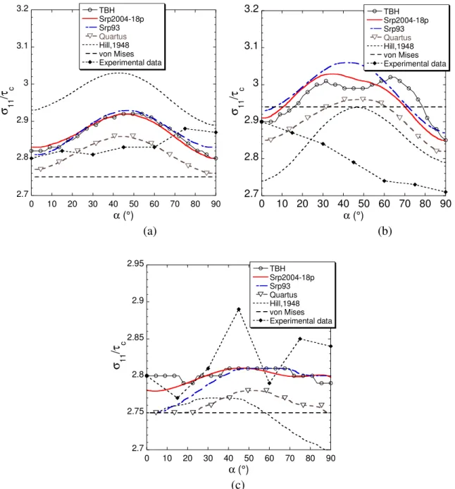
5.1 Crystallographic texture-based identification Figure 1 and (a) (b) (c) 2.7 2.8 2.9 3 3.1 3.2 0 10 20 30 40 50 60 70 80 90 TBH Srp2004-18p Srp93 Quartus Hill,1948 von Mises Experimental data σ 1 1 /τ c α (°) 2.7 2.8 2.9 3 3.1 3.2 0 10 20 30 40 50 60 70 80 90 TBH Srp2004-18p Srp93 Quartus Hill,1948 von Mises Experimental data σ 11 /τ c α (°) 2.7 2.75 2.8 2.85 2.9 2.95 0 10 20 30 40 50 60 70 80 90 TBH Srp2004-18p Srp93 Quartus Hill,1948 von Mises Experimental data σ 1 1 /τ c α (°)
Figure 2 show an example of the anisotropy of the r-value and yield stresses (normalized by the critical resolved shear stress
τ
c) predicted when the micromechanical-based adjustmentprocedure is used on different materials. The experimental data obtained using off-axis uniaxial tensile tests, are added in the figures for comparison. With regard to yield loci (normalized with the critical shear stress
τ
c, Figure 3), the predictions of the quadraticpotentials are clearly improved by the Srp2004-18p and Quartus potentials. However, discrepancies are observed in the prediction of the r-value specifically when the anisotropic
texture-based approach, the r-values are not used for the parameter identification and thus can be used for validation purposes.
(a) (b) (c) 1 1.5 2 2.5 3 0 10 20 30 40 50 60 70 80 90 TBH Srp2004-18p Srp93 Quartus Hill,1948 von Mises Experimental data r( α ) α(°) 0.2 0.4 0.6 0.8 1 1.2 0 10 20 30 40 50 60 70 80 90 TBH Srp2004-18p Srp93 Quartus Hill,1948 von Mises Experimental data r( α ) α(°) 0.7 0.8 0.9 1 1.1 1.2 0 10 20 30 40 50 60 70 80 90 TBH Srp2004-18p Srp93 Quartus Hill,1948 von Mises Experimental data r( α ) α(°)
Figure 1 r-value predictions for several potentials when crystallographic texture-based identification is adopted. (a) IF mild steel DC06, (b) Aluminium alloy AA6022-T43, (c) Dual Phase DP600 steel.
(a) (b) (c) 2.7 2.8 2.9 3 3.1 3.2 0 10 20 30 40 50 60 70 80 90 TBH Srp2004-18p Srp93 Quartus Hill,1948 von Mises Experimental data σ 11 /τ c α (°) 2.7 2.8 2.9 3 3.1 3.2 0 10 20 30 40 50 60 70 80 90 TBH Srp2004-18p Srp93 Quartus Hill,1948 von Mises Experimental data σ 1 1 /τ c α (°) 2.7 2.75 2.8 2.85 2.9 2.95 0 10 20 30 40 50 60 70 80 90 TBH Srp2004-18p Srp93 Quartus Hill,1948 von Mises Experimental data σ 1 1 /τ c α (°)
Figure 2 Yield stresses predictions for several potentials when crystallographic texture-based identification is adopted. (a) IF mild steel DC06, (b) Aluminium alloy AA6022-T43, (c) Dual Phase DP600 steel.
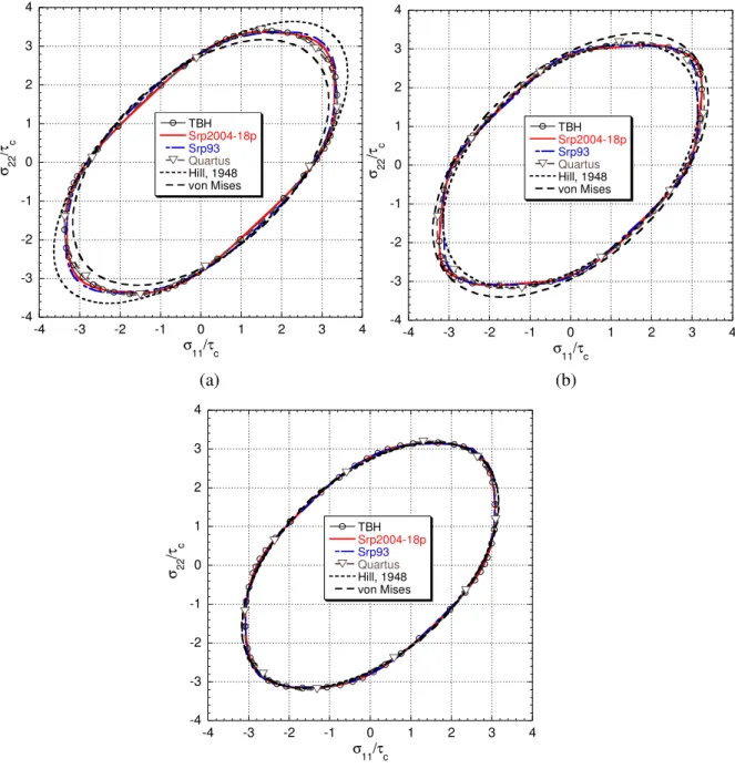
(a) (b) (c) -4 -3 -2 -1 0 1 2 3 4 -4 -3 -2 -1 0 1 2 3 4 TBH Srp2004-18p Srp93 Quartus Hill, 1948 von Mises σ 2 2 /τ c σ 11/τc -4 -3 -2 -1 0 1 2 3 4 -4 -3 -2 -1 0 1 2 3 4 TBH Srp2004-18p Srp93 Quartus Hill, 1948 von Mises σ 2 2 /τ c σ 11/τc -4 -3 -2 -1 0 1 2 3 4 -4 -3 -2 -1 0 1 2 3 4 TBH Srp2004-18p Srp93 Quartus Hill, 1948 von Mises σ 2 2 /τ c σ11/τc
Figure 3 Yield surface predictions for several potentials when crystallographic texture-based identification is adopted (computation carried out with
{
011 11 1 and}
{
112 11 1 slip families for bcc materials and}
{
11 1 011 slip family for fcc materials). (a) IF mild steel DC06, (b) Aluminium alloy AA6022-T43, (c) Dual}
Potentials
Mechanical data-based Crystallographic data-based
AA6022-T43 AA2090-T3 AA2008-T4 DP600 AA6022-T43 DC06 DP600 Sr p 2 0 0 4 -1 8 p b1 0.4212 0.3899 0.9253 -0.3880 0.3174 0.9552 0.1341 b2 -0.7992 0.6832 1.2680 0.8800 0.0152 0.9893 0.5141 b3 1.0704 0.9090 1.3418 1.2600 0.7568 1.2842 1.1634 b4 -0.1444 1.0109 1.1949 0.6980 0.2410 1.2377 1.0563 b5 -0.0860 1.1323 0.3638 0.9020 0.4022 1.2117 0.6356 b6 -0.4176 0.6264 0.3418 0.7440 0.2673 1.2144 0.5963 b7 1.0120 1.0020 1.0600 1.0000 0.7076 1.3448 0.7458 b8 1.1040 0.5635 0.9000 1.0000 0.4440 1.1439 -0.0087 b9 0.9611 1.0703 1.2771 1.0000 0.1820 1.3870 0.5735 b10 1.4010 1.3692 0.7990 1.1600 1.3642 0.5695 1.1936 b11 1.0898 0.7683 0.9553 0.6360 1.4038 -0.4002 1.3097 b12 0.8842 1.4545 0.7286 0.7700 1.4569 0.6464 1.2247 b13 1.0281 0.6826 1.0405 0.9170 1.4284 -0.2051 1.1146 b14 0.9415 0.9383 0.1169 1.1600 1.5882 -0.1529 1.3339 b15 1.0724 1.1074 0.5947 0.4570 1.5605 -0.7111 1.0895 b16 1.0120 1.0020 1.0600 1.0000 1.4803 -0.4046 1.1794 b17 1.1040 0.5635 0.9000 1.0000 1.6225 -0.8189 1.5432 b18 1.1758 0.5083 0.6863 1.0800 1.7888 0.5119 1.3890 µ 1.4010 1.3333 1.3333 1.7800 1.2640 1.4990 1.5171 Sr p 9 3 c1 0.8956 0.9056 0.8072 0.9920 0.9522 1.0968 1.0283 c2 1.0089 0.9138 0.9663 0.9710 0.9903 1.0797 0.9924 c3 1.0143 1.0606 1.0129 1.0000 1.0099 0.9263 1.0077 c4 1.0000 1.0000 1.0000 1.0000 1.1031 0.9221 1.0064 c5 1.0000 1.0000 1.0000 1.0000 1.0731 0.9391 1.0330 c6 1.0352 0.8245 0.9958 1.0300 1.0756 1.0307 1.0260 µ 1.3333 1.3333 1.3333 1.5000 1.3296 1.6063 1.5517 Q u a rt u s α1 3.3262 3.0617 3.1603 3.2000 3.2751 3.4549 3.2096 α2 3.1141 2.9778 2.8008 3.2400 3.1622 3.5051 3.3014 α3 3.2660 3.2660 3.2660 3.2660 3.7685 2.9584 3.2765 α4 3.2660 3.2660 3.2660 3.2660 3.6904 3.0204 3.3644 α5 3.6043 2.4120 3.4445 3.3700 3.6739 3.2601 3.3360 α6 6.4118 5.6264 6.0438 6.2600 6.5023 6.8453 6.3126 α7 6.2361 6.4392 5.5018 6.2200 6.2727 6.9710 6.5265 α8 9.5573 9.6742 8.8248 9.3100 9.5990 9.9496 9.5735 α9 6.5320 6.5320 6.5320 6.5320 6.5111 6.6972 6.3561 α10 6.5320 6.5320 6.5320 6.5320 6.9435 6.4091 6.4937 α11 5.9286 5.9475 6.1642 6.4800 6.4006 6.9840 6.5316 α12 6.5320 6.5320 6.5320 6.5320 6.8686 6.4387 6.5589 α13 6.5320 6.5320 6.5320 6.5320 6.1979 6.8756 6.5502 α14 6.0664 5.8206 5.6784 6.5000 6.5754 6.9564 6.5461 α15 6.5320 6.5320 6.5320 6.5320 6.8321 5.7396 6.5308 α16 6.5320 6.5320 6.5320 6.5320 6.7905 6.6667 6.3481 α17 6.5320 6.5320 6.5320 6.5320 6.5335 6.7797 6.6062 α18 6.5320 6.5320 6.5320 6.5320 7.0078 6.6227 6.5294 α19 6.5320 6.5320 6.5320 6.5320 6.6083 6.8739 6.7160 α20 5.5229 4.2424 5.1755 6.3900 5.9970 7.5806 6.5379 α21 3.2660 3.2660 3.2660 3.2660 0.6137 -1.1834 -0.2269 α22 3.2660 3.2660 3.2660 3.2660 0.1261 -0.8967 0.1035 H il l’ 4 8 F 1.0214 0.1713 0.1905 0.6380 0.8518 1.2413 0.9886 G 0.9529 0.1351 0.1146 0.6380 0.7869 1.3007 1.0636 H 0.9489 1.7023 1.4655 0.6610 1.0021 1.1085 1.0185 L 3.0000 0.3200 0.3200 0.6670 2.4324 3.8472 2.9199 M 3.0000 4.3478 2.6674 0.6670 2.3924 3.1423 2.9424 N 2.9031 4.3956 4.5251 0.7320 3.0684 2.6108 3.0481 von Mises 0.9290 1.0599 0.8204 0.6430 0.9049 1.1903 1.0593
Table 1 Material parameters of the different plastic potentials for the materials under investigation, as identified with the two methods. Yield stresses normalized by σ0.
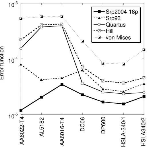
The sets of material parameters obtained in the current investigation are summarized in Table 1. Figure 4 shows the comparison of the error function values, (Eq.(18)), obtained after the identification of the investigated potentials for the different BCC and FCC materials. The conclusions drawn in (Bacroix et al., 2003) are again verified for the materials tested in this work: Srp93 provides better predictions than Quartus for aluminium alloys, while Quartus does better for all steels. In contrast, the recent Srp2004-18p potential provides a better fit than both Srp93 and Quartus in all cases. The main interest of the texture-based identification procedure is that it provides such consistent comparison between different potentials. The above conclusions have been found for more than ten different aluminium alloys and ten different steel sheets. Thus one may consider that, among the potentials considered in this work, Srp2004-18p has great chances to provide the best fit for virtually any metal sheet in these categories.
10
-510
-410
-3Srp2004-18p
Srp93
Quartus
Hill
von Mises
A
L
5
1
8
2
A
A
6
0
2
2
-T
4
A
A
6
0
1
6
-T
4
D
C
0
6
H
S
L
A
-3
4
0
/1
H
S
L
A
3
4
0
/2
D
P
6
0
0
E
rr
o
r
fu
n
c
ti
o
n
Figure 4 Error function for several BCC (IF mild steel DC06, Dual Phase steel DP600 and micro-alloyed steels HSLA with different thicknesses) and FCC materials (Al-Mg AA5182-O, Al-Mg-Si AA6022-T4 and
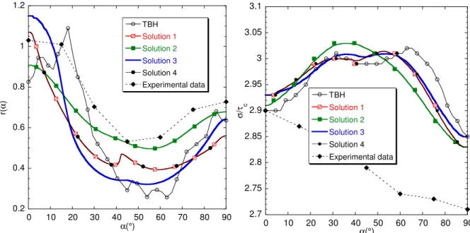
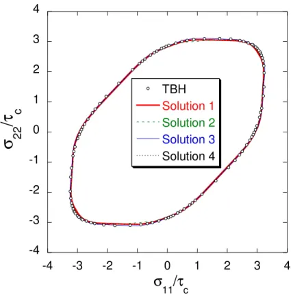
The sensitivity of the predicted results to some numerical aspects (initial guess for the parameters, objective function weights, the number of iterations…) has been carefully investigated in this work. Although the adopted algorithm is known to be robust and efficient, it is sensitive to the initial parameters guess, like most of the minimization algorithms seeking for the closest local minimum. Figure 5 and 6 present the sensitivity of the material parameters identification to the initial introduced solution for fixed β1 and q parameters. As
one can see, the impact of the initial set of parameters on the shape of the yield surface is negligible (Figure 6). However, when the r-value or the yield stress anisotropies are checked, some differences are found. This suggests that these two important measures of anisotropy could also be included in the objective function for a better controlled identification. Nevertheless, it should be noted that the r-values predicted by the Taylor model are less reliable than the yield surface itself. In the example from Figure 5, the impact of the initial guess is smaller than the gap between the micromechanical and the experimental r-values.
0.2 0.4 0.6 0.8 1 1.2 0 10 20 30 40 50 60 70 80 90 TBH Solution 1 Solution 2 Solution 3 Solution 4 Experimental data r( α ) α(°) 2.7 2.75 2.8 2.85 2.9 2.95 3 3.05 3.1 0 10 20 30 40 50 60 70 80 90 TBH Solution 1 Solution 2 Solution 3 Solution 4 Experimental data σ /τ c α(°)
Figure 5 Aluminium alloy AA6022-T43: Sensitivity analysis to the initial guess of parameters for crystallographic texture-based identification carried out on Srp2004-18p strain rate potential with β1 = 1 and q
-4 -3 -2 -1 0 1 2 3 4 -4 -3 -2 -1 0 1 2 3 4 TBH Solution 1 Solution 2 Solution 3 Solution 4
σ
2 2/τ
cσ
11/τ
cFigure 6 Aluminium alloy AA6022-T43: Sensitivity analysis to the initial guess of parameters for crystallographic texture-based identification carried out on Srp2004-18p strain rate potential.
When crystallographic-data-based identification is adopted, the cost function uses 80,000 “experimental values” on the yield surface, Eq. (18). A specific weighting factor wi, Eq. (19)
for every strain rate direction can be imposed. This factor is intended to give a smaller weight to the through-thickness shear modes (wi = 1 when the components of the plastic strain rate
tensor lie in the plane of the sheet and wi = 1 - β1 for purely through-thickness shear modes).
Thus β1 = 1 allows for a complete discrimination of the later deformation modes. When β1 ≠ 0,
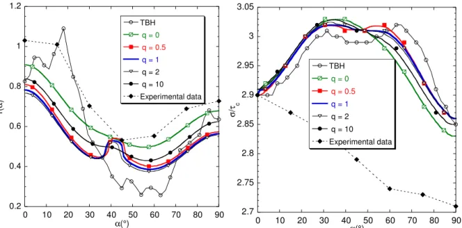
the q parameter intensifies the effect of β1. With regard to the numerical results in Figure 7
and Figure 8, the same conclusions can be drawn as for the sensitivity to the initial parameter guess: the impact on the yield surface is subtle, while there is a significant sensitivity of the Hill coefficients of anisotropy and uniaxial tensile yield stress to the weights adopted in the cost function. In our comparative studies, both the coefficients β1 and q have been kept equal
to one for consistent comparisons. No need to say here that such sensitivity aspects were already reported in published researches relative to the optimization algorithm. However, the general trends reported later were obtained taking under consideration such sensitivity studies.
0.2 0.4 0.6 0.8 1 1.2 0 10 20 30 40 50 60 70 80 90 TBH q = 0 q = 0.5 q = 1 q = 2 q = 10 Experimental data r( α ) α(°) 2.7 2.75 2.8 2.85 2.9 2.95 3 3.05 0 10 20 30 40 50 60 70 80 90 TBH q = 0 q = 0.5 q = 1 q = 2 q = 10 Experimental data σ /τ c α(°)
Figure 7 Aluminium alloy AA6022-T43: Sensitivity analysis to the value of q, for crystallographic texture-based identification carried out on Srp2004-18p strain rate potential with β1 = 1.
0.2 0.4 0.6 0.8 1 1.2 0 10 20 30 40 50 60 70 80 90 TBH β 1 = 0 β 1 = 0.3 β 1 = 0.5 β 1 = 0.6 β 1 = 0.8 β 1 = 1 Experimental data r( α ) α(°) 2.7 2.75 2.8 2.85 2.9 2.95 3 3.05 0 10 20 30 40 50 60 70 80 90 TBH β 1 = 0 β 1 = 0.3 β 1 = 0.5 β 1 = 0.6 β 1 = 0.8 β 1 = 1 Experimental data σ 1 1 /τ c α(°)
Figure 8 Aluminium alloy AA6022-T43: Sensitivity analysis to the value of β1, for crystallographic
texture-based identification carried out on Srp2004-18p strain rate potential with q = 1.
5.2 Mechanical data-based identification
Figure 9 and Figure 10 depict an example of the best fit predictions obtained with the five potentials when mechanical data-based adjustments are used. The predictions of the quadratic potentials are clearly improved by the three other potentials (Srp93, Srp2004-18p and
11). When mechanical data-adjustment approach is adopted, Srp2004-18p seems to exhibit more flexibility in accurately describing the yielding behaviour of the examined aluminium alloys (e.g. Figure 9, Figure 12 and
Figure 13). Consequently, the comparison of the different potentials’ flexibility leads to similar conclusions as when the texture-based identification is used. However, Quartus appears here to perform better than Srp93 even for aluminium alloys, in terms of objective function. In fact, a more careful examination of the results reveals that for aluminium alloys, the best-fit set of parameters for Quartus often leads to a non-convex yield surface, as illustrated in Figure 14. The major difficulty for this potential appears to be the simultaneous fit of both the uniaxial tensile experiments and the biaxial one. Reducing the weight of the biaxial point in the cost function leads to acceptable solutions (convex yield surface). This is how the results for Quartus have been obtained in the figures above. Yet, the corresponding cost functions cannot be compared anymore to the other ones since the considered weights are different. It is noteworthy that with the texture-based identification, no loss of convexity has been detected for Quartus. This is attributed to the use of numerous, evenly distributed, equally weighted reference points for the identification, which prevent any unrealistic distortion of the yield surface.
0.92 0.94 0.96 0.98 1 1.02 1.04 0 15 30 45 60 75 90 Srp2004-18p Srp93 Quartus Hill48 von Mises Experimental data σ 1 1 /σ b α(°) 0.5 0.6 0.7 0.8 0.9 1 1.1 0 15 30 45 60 75 90 Srp2004-18p Srp93 Quartus Hill48 von Mises Experimental data r( α ) α(°)
Figure 9 Aluminium alloy AA6022-T43: Yield stress and r-value predictions for several potentials when mechanical data-based identification is adopted.
-1.5 -1 -0.5 0 0.5 1 1.5 -1.5 -1 -0.5 0 0.5 1 1.5 Srp2004-18p Srp93 Quartus Hill, 1948 von Mises Experimental data
σ
2 2/σ
bσ
11/σ
bFigure 10 Aluminium alloy AA6022-T43: Yield surface predictions for several potentials when mechanical data -based identification is adopted.
10-5 10-4 10-3 10-2 10-1 100 Srp2004-18p Srp93 Quartus Hill Von mises A A2 0 9 0 -T 3 A A2 0 0 8 -T 4 A A6 0 2 2 -T 4 3 D P 6 0 0
0 0.2 0.4 0.6 0.8 1 1.2 1.4 1.6 0 10 20 30 40 50 60 70 80 90 Srp2004-18p Srp93 Quartus Hill,1948 von Mises Experimental data r( α ) α(°) 0.75 0.8 0.85 0.9 0.95 1 1.05 0 10 20 30 40 50 60 70 80 90 Srp2004-18p Srp93 Quartus Hill,1948 von Mises Experimental data σ 1 1 /σ 0 α (°)
Figure 12 Al-Li aluminium alloy AA2090-T3: Yield stress and r-value predictions for several potentials when mechanical data-based identification is adopted.
0.4 0.5 0.6 0.7 0.8 0.9 1 1.1 0 10 20 30 40 50 60 70 80 90 Srp2004-18p Srp93 Quartus Hill,1948 von Mises Experimental data r( α ) α(°) 0.84 0.86 0.88 0.9 0.92 0.94 0.96 0.98 1 1.02 0 10 20 30 40 50 60 70 80 90 Srp2004-18p Srp93 Quartus Hill,1948 von Mises Experimental data σ 1 1 /σ 0 α (°)
Figure 13 Aluminium alloy AA2008-T4: Experimental yield stress and r-value and predictions based on several potentials. Mechanical data-based identification.
-1.2 -0.8 -0.4 0 0.4 0.8 1.2 -1.2 -0.8 -0.4 0 0.4 0.8 1.2 Quartus (w r1 = 5) Quartus (w r1 = 1) Experimental data
σ
2 2/σ
0σ
11/σ
0Figure 14 Predictions of the Quartus potential for aluminium alloy AA2090-T3: best fit results (thin line) and acceptable solution that does not violate convexity (thick line). The parameter wr1 corresponds to the weight
affected to the équibiaxiale yield stress as defined in Eq. (20).
When the material exhibits weak in-plane anisotropy (e.g. the dual phase steel DP600 in this work), the identified yield surfaces obtained with the different potentials are very close to the von Mises yield surface. Nonetheless, the predicted Hill coefficients of anisotropy can be very different as indicated by Figure 1 (c) for DP600 steel. For this material, when the mechanical data-based approach is adopted, a significant improvement in the predicted Hill coefficients of anisotropy is achieved (Figure 15) with general yield loci close to the von Mises surface (Figure 16). A careful inspection of the predicted yield locus using the two identification strategies clearly indicates that the normal to the yield surfaces can be very different (Figure 17, a). These differences can be even larger when the in-plane anisotropy become more pronounced as for the AA6022-T43 material (Figure 17, b).
0.75 0.8 0.85 0.9 0.95 1 1.05 0 10 20 30 40 50 60 70 80 90 Srp2004-18p Srp93 Quartus Hill,1948 von Mises Experimental data r( α ) α(°) 0.97 0.98 0.99 1 1.01 1.02 1.03 1.04 0 10 20 30 40 50 60 70 80 90 Srp2004-18p Srp93 Quartus Hill,1948 von Mises Experimental data σ 1 1 /σ 0 α (°)
Figure 15 Dual Phase DP600 steel: Experimental yield stress and r-value and predictions based on several potentials. Mechanical data-based identification.
-1.5 -1 -0.5 0 0.5 1 1.5 -1.5 -1 -0.5 0 0.5 1 1.5 Srp2004-18p Srp93 Quartus Hill, 1948 von Mises Experimental data
σ
2 2/σ
0σ
11/σ
0Figure 16 Dual Phase DP600 steel: Yield surface predictions for several potentials when mechanical data -based identification is adopted.
-1.5 -1 -0.5 0 0.5 1 1.5 -1.5 -1 -0.5 0 0.5 1 1.5 (a) DP600 Mechanical data-based
Crystallographic texture data-based
σ 2 2 /σ 0 σ 11/σ0 -1.5 -1 -0.5 0 0.5 1 1.5 -1.5 -1 -0.5 0 0.5 1 1.5 (b) AA6022-T43 Mechanical data-based
Crystallographic texture data-based
σ 2
2
/σ 0
σ
11/σ0
Figure 17 Determined Srp2004-18p yield surface using different strategies of material parameters identification.
Depending on the procedure used to identify the parameters, the resulting predictions of plastic anisotropy are slightly different. It can be observed that when mechanical test data is used for the identification, the predictions of the r-value and yield stress anisotropy with all the non-quadratic potentials are closer to each other while the scatter in the prediction of the yield surface is more significant (Figure 10). On the contrary, a larger scatter in r-values and yield stress anisotropy predictions is obtained with the texture-based identification (Figure 1-b
and (a) (b) (c) 2.7 2.8 2.9 3 3.1 3.2 0 10 20 30 40 50 60 70 80 90 TBH Srp2004-18p Srp93 Quartus Hill,1948 von Mises Experimental data σ 1 1 /τ c α (°) 2.7 2.8 2.9 3 3.1 3.2 0 10 20 30 40 50 60 70 80 90 TBH Srp2004-18p Srp93 Quartus Hill,1948 von Mises Experimental data σ 1 1 /τ c α (°) 2.7 2.75 2.8 2.85 2.9 2.95 0 10 20 30 40 50 60 70 80 90 TBH Srp2004-18p Srp93 Quartus Hill,1948 von Mises Experimental data σ 11 /τ c α (°)
Figure 2-b). Figure 16 and Figure 18 provide very typical examples, where the prediction of the plane strain tension stresses is very different from a potential to the other, while the mechanical-test based anisotropy is predicted almost identically.
The origin of this behaviour is again the discrepancy in the number, type and location of the reference data used for the parameter fit in the two identification procedures. Figure 19 shows the respective reference (experimental) data used in both cases. The texture-based identification makes use of an extensive, evenly-distributed set of reference points (plastic
including both stress values and plastic strain rate directions. More specifically, the plane strain tension area is poorly represented in the commonly used set of experiments – which may explain e.g. the scatter in Figure 18 corresponding to this area. However, diversifying the mechanical tests is an extremely challenging task.
-1.5 -1 -0.5 0 0.5 1 1.5 -1.5 -1 -0.5 0 0.5 1 1.5 Srp2004-18p Srp93 Quartus Experimental data σ 2 2 /σ 0 σ 11/σ0
Figure 18 Yield surface predictions for several potentials when mechanical data -based identification is adopted: Aluminium alloy AA2008-T4.
-1.5 -1 -0.5 0 0.5 1 1.5 -1.5 -1 -0.5 0 0.5 1 1.5 σ 2 2 /σ 0 σ 11/σ0 Texture points
Uniaxiale tensile tests
Shear tests
Figure 19 Tri-component (σ11- σ22- σ12) normalised yield surface representation and location of the reference
One can easily duplicate the available tests by means of the micromechanical model, so that similar data and the same procedure can be used for the identification. Figure 1 and
(a) (b) (c) 2.7 2.8 2.9 3 3.1 3.2 0 10 20 30 40 50 60 70 80 90 TBH Srp2004-18p Srp93 Quartus Hill,1948 von Mises Experimental data σ 1 1 /τ c α (°) 2.7 2.8 2.9 3 3.1 3.2 0 10 20 30 40 50 60 70 80 90 TBH Srp2004-18p Srp93 Quartus Hill,1948 von Mises Experimental data σ 11 /τ c α (°) 2.7 2.75 2.8 2.85 2.9 2.95 0 10 20 30 40 50 60 70 80 90 TBH Srp2004-18p Srp93 Quartus Hill,1948 von Mises Experimental data σ 1 1 /τ c α (°)
Figure 2 show the r-value and yield stress anisotropy as measured and as predicted by the Taylor model, for three materials. It is obvious that for some materials, the Taylor model leads to poor predictions of these anisotropy indicators. Consequently, in such situations the texture-based identification method does not provide a good accuracy, unless a more accurate micromechanical description of the plastic anisotropy is obtained. For this purpose, different micromechanical models (e.g. self-consistent models, finite element polycrystalline models etc.) could be used in the framework of the current approach, without any limitation.
The texture-based identification procedure can also be penalized in terms of final accuracy if an equal weight is considered for all the reference points in the 5D deviatoric plastic strain rate space. Indeed, while this guarantees a consistent fit of the whole space of possible straining modes, practical sheet forming applications exhibit near plane-stress loading situations. Thus, one should prescribe lower weights to the out-of-plane shear terms, e.g. with the weight function (Eq.(19)).
5.3 Combined strategy for material parameters identification
When both mechanical test data and crystallographic texture are available, one can combine the advantages of the two parameter identification methods by combining the two error functions in a single one:
(
)
2 Tex 2 Mech
F= β F + 1− β F , (21)
where FTex is defined by Eq. (19) and FMech by Eq.(20). This approach has been applied here
for the AA6016-T4 aluminium alloy, by using the Srp93 potential. The Taylor-predicted data is combined with experimentally determined shear yield stresses. As shown in Figure 20, when only the texture-based function is used (e.g. β2=1) the anisotropy of the experimental
shear stresses is very poorly reproduced by the identified parameters. Decreasing the value of β2 allows for a progressive improvement of the fit, until the results of the
mechanical-test-based identification procedure are completely recovered. In such cases, when the Taylor model does not accurately describe the r-values and/or uniaxial yield stresses, one should use the mechanical test data to identify as many parameters as possible. Nevertheless, several parameters cannot be identified with the experimental data alone; instead of arbitrarily keeping their values to the isotropic case, using the Taylor model contributes to improve the final identification result.
58 60 62 64 66 68 70 0 30 60 90 120 150 Experimental β 2 = 1 β 2 = 0.5 β 2 = 0.1 S h e a r s tr e s s [ M P a ] α(°)
Figure 20 Aluminium alloy AA6016-T4: experimental and predicted yield stress anisotropy, using the combined identification.
6. Conclusion
The present work clearly highlights the impact of the identification method (using either texture data or mechanical tests) on the resulting accuracy. Overall, the advantage of the recent Srp2004-18p potential is demonstrated for a wide range of initial material anisotropy. Nonetheless, the fourth-order series expansion Quartus still remains attractive for the present FCC and especially BCC materials. The comparison of the two identification strategies, using either experimental or micromechanical data, reveals that introducing a combined adjustment making use of the two procedures would probably enhance the description of the initial anisotropy. However, the practical use of the texture-based identification heavily relies on the ability of the micromechanical model to describe accurately the plastic anisotropy of the material. The different potentials studied in this work have been implemented in the finite element code Abaqus. Ongoing work will focus on the impact of the identification strategy (micromechanical-based or mechanical data-based) on the prediction of the earing profile of a cup after drawing of a circular blank.
REFERENCES
Arminjon M., Bacroix B., 1991. On plastic potentials for anisotropic metals and their derivation from the texture function, Acta Mechanica 88, 219-243.
Arminjon M., Bacroix B., Imbault D., Raphanel J. L., 1994. A fourth-order plastic potential for anisotropic metals and its analytical calculation from the texture function, Acta Mechanica 107, 33-51.
Bacroix B., Balan T., Bouvier S., Teodosiu C.,2003. Identification of plastic potentials by inverse method, In: Proc. 6th Int. Esaform Conf., Salerno, Italy, April 28-30 2003, pp. 347-350.
Balan T., Bacroix B., Teodosiu C., 2000. On the identification of strain rate potentials using both texture data and mechanical tests, Proc. of TPR 2000, Cluj-Napoca (Romania), 81-93. Banabic D., 2001. Anisotropy of sheet metals. In: Banabic, D. (Ed.), Formability of Metallic
Materials. Springer, Berlin, pp. 119–172.
Banabic D., Kuwabara T., Balan T., Comsa D.S., Julean D., 2003. Non-quadratic yield criterion for orthotropic sheet metals under plane-stress conditions. Int. J. Mech. Sci. 45, 797-811
Barlat F., Lege D.J., Brem J.C., 1991. A six-component yield function for anisotropic materials, Int. J. Plasticity 7, 693-712.
Barlat F. and Chung K., 1993. Anisotropic potentials for plastically deformation metals. Modelling Simul. Mater. Sci. Engng. 1, 403-416.
Barlat F., Chung K., Richmond O., 1993. Strain rate potential for metals and its application to minimum plastic work path calculations, Int. J. Plasticity 9, 51-63.
Barlat F., Chung K., Richmond O., 1994. Anisotropic plastic potentials for polycrystals and application to the design of optimum blank shapes in sheet forming. Metallurgical and Materials Transactions A 25, 1209-1216.
Barlat F., Maeda Y., Chung K., Yanagawa M., Brem J. C., Hayashida Y., Lege D. J., Matsui K., Murtha S. J., Hattori S., Becker R. C., Makosey S., 1997. Yield function development for aluminium alloy sheets, J. Mech. Phys. Solids 45, 1727-1763.
Barlat F., Brem J.C., Yoon J.W., Chung K., Dick R.E., Lege D.J., Pourboghrat F., Choi S.-H., Chu E., 2003. Plane stress yield function for aluminum alloy sheet. Part I: Theory. Int. J. Plasticity 19, 1297–1319.
Barlat F., Cazacu O., Życzkowski M., Banabic D., Yoon J.W., 2004. Yield surface plasticity and anisotropy. In: Raabe, D., Chen, L.-Q., Barlat, F., Roters, F. (Eds.), Continuum Scale
Simulation of Engineering Materials Fundamentals – Microstructures – Process Applications. WILEY–VCH Verlag, Berlin GmbH, pp. 145–177.
Barlat F. and Chung K., 2005, Anisotropic strain rate potential for aluminium alloy plasticity, Proc. of The 8th Esaform Conference on Material Forming, Cluj-Napoca, Romania, 27-29 April 2005, pp.415-418.
Barlat F., Aretz H., Yoon J.W., Karabin M.E., Brem J.C. and Dick R.E., 2005. Linear transfomation-based anisotropic yield functions. Int. J. Plasticity, 21, 1009-1039.
Berveiller M. and Zaoui A., 1979. An extension of the self-consistent scheme to plastically flowing polycrystals. J. Mech. Phys. Solids, 26, 325-344.
Bishop J.F.W., Hill R., 1951. A theory of the plastic distorsion of a polycrystalline aggregate under combined stress, Phil. Mag. 42, 414-427.
Budiansky B., 1984. Anisotropic plasticity of plane-isotropic sheets, in: Mechanics of Material Behavior, Dvorak G.J. and Shield R.T. (eds.), Elsevier, 15-29.
Cazacu O., Barlat F., 2001. Generalization of Drucker’s yield criterion to orthotropy. Math. Mech. Solids 6, 613–630.
Cazacu O., Barlat F., 2003. Application of representation theory to describe yielding of anisotropic aluminum alloys. Int. J. Eng. Sci. 41, 1367–1385.
Chung K., Lee S.Y., Barlat F., Keum Y.T., and Park J.M., 1996. Finite element simulation of sheet forming based on a planar anisotropic strain rate potential. Int. J. Plasticity 12(1), 93-115.
Chung K., Barlat F., Brem J.C., Lege D.J., Richmond O., 1997. Blank shape design for a planar anisotropic sheet based on ideal forming design theory and FEM analysis. Int. J. Mech. Sci., 39(1), 105-120.
Chung K., Barlat F., Richmond O., Yoon, J.W., 1999. Blank design for a sheet forming application using the anisotropic strain rate potential Srp98. The integration of Material, Process and Product Design, Zabaras et al. (Eds.), Balkema, Rotterdam.213-219.
Dennis J.E. and Schnabel R.B., 1983. Numerical methods for unconstrained optimization and non-linear equations. Prentice Hall, Englewood Cliffs, NJ, USA.
Ferron G., Makkouk R., Morreale J., 1994. A parametric description of orthotropic plasticity in metal sheets, Int. J. Plasticity 10, 431-449.
Gotoh M., 1977. A theory of plastic anisotropy based on a yield function of fourth order, Int. J. Mech. Sci. 19, 505-520.
Hill R., 1948. A theory of the yielding and plastic flow of anisotropic metals, Proc. Royal Soc. A 193, 281-297.
Hill R., 1979. Theoretical plasticity of textured aggregates, Math. Proc. Cambr. Phil. Soc. 85, 179-191.
Hill R., 1987. Constitutive dual potentials in classical plasticity, J. Mech. Phys. Solids 35, 22-33.
Hill R., 1993. A user-friendly theory of orthotropic plasticity in sheet metals, Int. J. Mech. Sci. 35, 19-25.
Hosford W.F., 1972. A generalised isotropic yield function, J. Appl. Mech. 39, 607-619. Karafillis A.P., Boyce M.C., 1993. A general anisotropic yield criterion using bounds and a
transformation weighting tensor, J. Mech. Phys. Solids 41, 1859-1886.
D. Kim, F. Barlat, S. Bouvier, M. Rabahallah, T. Balan, K. Chung, 2007. Non-quadratic anisotropic potential based on linear transformation of plastic strain rate, Int. J. Plasticity, in press.
Kuwabara T., Ikeda S. and Kuroda K., 1998, Measurement and analysis of differential work hardening in cold-rolled steel sheet under biaxial tension, J. Mat. Proc. Tech., 80-81, 517-523.
Lege D.J., Barlat F. and Brem J.C.. 1989, Characterization and modeling of the mechanical behavior and formability of a 2008-T4 sheet sample. Int. J. Mech. Sci., 31, 549-563.
Pöhlandt K., Banabic D., Lange K., 2002. Equi-biaxial anisotropy coefficient used to describe the plastic behavior of sheet metal, In: Prof. ESAFORM 2002 Conference, Krakow, Poland, 723-727.
Rabahallah M., Bacroix B., Bouvier S., Balan T., 2006. Crystal plasticity based identification of anisotropic strain rate potentials for sheet metal forming simulation, III European Conference on Computational Mechanics, C.A. Mota Soares et.al. (Eds.), Lisbon, Portugal. Savoie J. and MacEwen S.R., 1996. A sixth order inverse function for incorporation of crystallographic texture into predictions of properties of aluminium sheet. In Textures and Microstructures, 26/27, 495-512.
Taylor G.I., 1938. Plastic strain in metals, J. Inst. Metals 62, 307-324.
Van Houtte P., Mols K., Van Bael, A., Aernoudt E., 1989. Application of yield loci calculated from texture data, Textures Microstruct. 11, 23-39.
Van Houtte P. and Van Bael A., Winters J., Aernoudt E., Hall F., Wang N., Pillinger I., Hartley P. and Sturgess C.E.N., 1992, Modelling of complex forming processes. In Andersen S.I. et al. (Eds.), Modeling of Plastic Deformation and Its Engineering Applications, Proc. 13th Risø International Symposium on Materials Science. Risø National Laboratory, Denmark, pp. 161-172.
Van Houtte P. and Van Bael A., 2004. Convex plastic potentials of fourth and sixth rank for anisotropic materials, Int. J. Plasticity 20, 1505-1524.
Vegter D., 1991. On the plastic behaviour of steel during sheet forming, PhD Thesis, Univ. Twente
Yoon J.W., Song I.S., Yang D.Y., Chung K., Barlat F., 1994. Finite element method for sheet forming based on an anisotropic strain rate potential and the convected coordinate system, Int. J. Mech. Sci., 37, 733-752.
Yu M.H., 2002. Advances in strength theories for materials under complex stress state in the 20th Century. Appl. Mech. Rev. 55, 198–218.
Ziegler H., 1977. An introduction to thermodynamics, North-Holland, Amsterdam.
Życzkowski M., 2001. Anisotropic yield conditions. In: Lemaitre, J. (Ed.), Handbook of Materials Behavior Models. Academic Press, San Diego, CA, pp. 155–165.