Effects of working parameters on the surface roughness in belt grinding process: the size-scale estimation influence

To cite this version :

Adrien VAN GORP, Maxence BIGERELLE, Mohamed EL MANSORI, Patrick GHIDOSSI, Alain IOST - Effects of working parameters on the surface roughness in belt grinding process: the sizescale estimation influence Int. J. Materials and Product Technology Vol. 38, n°1, p.1634 -2010

Effects of working parameters on the surface

roughness in belt grinding process: the size-scale

estimation influence

A. Van Gorp*

Arts et Metiers ParisTech, CNRS, LMPGM, 8, Boulevard Louis XIV,

59046 Lille Cedex, France E-mail: adrien.vangorp@ensam.eu *Corresponding author

M. Bigerelle

Laboratoire Roberval, UMR 6253, UTC/CNRS. UTC,

Centre de Recherches de Royallieu BP20529, 60205 Compiègne, France

E-mail: maxence.bigerelle@utc.fr

M. El Mansori and P. Ghidossi

Rue Saint Dominique BP 508 51006, Chalons-en-Champagne, France E-mail: mohamed.elmansori@ensam.eu E-mail: patrick.guidossi@ensam.eu

A. Iost

Arts et Metiers ParisTech, CNRS, LMPGM, 8, Boulevard Louis XIV,

59046 Lille Cedex, France Fax: 33(0)3 20 62 29 57 E-mail: alain.iost@ensam.eu E-mail: alain.iost@lille.ensam.fr

Abstract: This paper outlines a new method to evaluate roughness parameters

considering the scale used for their evaluation. Application is performed for grinding hardened steel with abrasive belts. Seven working variables are considered through a two-level experimental design. For all configurations, 30 surface profiles were recorded by tactile profilometry and rectified by a first degree B-spline fitting before calculating a set of current roughness parameters. The relevancy of each roughness parameter, to highlight process parameters influence, is then estimated for each scale by variance analysis. The results show that each influent input parameter is characterised by a related relevant evaluation length.

Keywords: roughness measurement; multi-scale analysis; variance analysis;

belt grinding process.

Reference to this paper should be made as follows: Van Gorp, A.,

Bigerelle, M., El Mansori, M., Ghidossi, P. and Iost, A. (2010) ‘Effects of working parameters on the surface roughness in belt grinding process: the size-scale estimation influence’, Int. J. Materials and Product Technology, Vol. 38, No. 1, pp.16–34.

Biographical notes: A. Van Gorp is a Doctor in Materials and Surfaces

Science, Engineer of ENSAM-ParisTech College (France). Field of interests: Tools processing, roughness, surfaces characterisation, polymer science. M. Bigerelle is a Professor in Materials Science, Engineer in Computer Sciences, PhD in Mechanics and Material Sciences (1999), Medical Expert in Biomaterials at the University Hospital Centre of Lille, Capacitation of Research. Directorship in Physical Sciences (2002). Field of interests: surfaces and interfaces morphological characterisation, multi-scale modelling, fractal and chaos, biomaterials and nanostructures. Director Assistant of the Materials Research Group in the Laboratory Roberval, UMR 6253, UTC/CNRS, Centre de Recherches de Royallieu, BP20529, 60205 Compiegne France.

M. El Mansori is a Professor in the Department of Mechanical Engineering and Manufacturing at ENSAM-ParisTech in Chalons, France, where much of his research interests lies in the thermo-mechanical and tribological performances of both metallic and composites materials when using various manufacturing processes. He is actually, the training leader of the ENSAM-ParisTech Machining Network. He has worked as research member in the ERMES Group (Nancy France) for five years on tribological behavior of many materials especially in the field of electrical and magnetised contacts. He was also a research fellow at the Center for Advanced Friction Studies at the Southern Illinois University (USA).

P. Guidossi is a Doctor in the Department of Mechanical Engineering and Manufacturing at ENSAM-ParisTech in Chalons, France. He mainly works with M. El Mansori on composites materials tooling and on manufacturing process optimisations.

A. Iost is a Professor of Metallurgy and Materials Science at ‘ENSAM Lille’ and leader of the team “Characterisation and Properties of Perisurfaces” at the Physical Metallurgy and Material Engineering Laboratory. The main fields of interests are the mechanical and morphological characterisation of the surfaces and interfaces.

1 Introduction

Precision tooling by turning and rectification of working surfaces is one of the most expansive steps of the production of mechanical parts. As a consequence, these operations are completed by other techniques like the belt grinding. The purpose is to reduce, on the one hand, the geometric defaults of part surface and, on the other hand, the structure defaults. One of the major advantages of belt grinding is the low level

of mechanical strain and microscopic cracks density since the surface temperature does not rise during the process. Moreover, this technique is simpler and less expensive.

The problem is that knowledge by manufacturers of this process is quite poor, compelling them to optimise the process in relation to their own experience. Some authors have already proposed works to make a characterisation of belt grinding process used in simulation models (Jourani et al., 2005; Zhang et al., 2005) and process automation (Huang et al., 2002). Some of them used an energetic point of view (Ghidossi et al., 2005) and others studied the influence of the process on residual stresses (Axinte et al., 2005), but most of them analysed the relationships between process conditions and roughness of the resulting surfaces through experimental designs (Rech and Moisan, 2003; Khellouki et al., 2005). The purpose of this paper is to improve this last approach by considering all the main process parameters and a more advanced definition of the roughness parameters taking in consideration their evaluation length. Moreover, we describe an original method to calculate roughness parameters using a first degree B-spline function fitting related to the evaluation length. Then, the problem is “What is the most relevant roughness parameter and its evaluation length to describe the effect of each process parameter and their interactions?” To answer, a variance analysis technique is used. Results give further information to explain mechanisms induced by the belt grinding process.

2 Experimental considerations

2.1 Grinding belt device

The testing bench is composed of a Bader type grinding belt device set-up on a conventional lathe. Consequently, the system have a horizontal structure which is currently used for the grinding belt superfinishing of crankshafts. To be sure of the reproductibility of the process, five bearings are tooled. Their dimensions are 54.78 mm in diameter and 30 mm in width (Figure 1). The belt is 20 mm wide. The tooling movement is composed of a tangential relative part displacement due to its rotation with regard to the belt one and an oscillation of the tooling arm in the axial direction of the tooled part.

2.2 Experiment design

The influence of the belt grinding process conditions on the resulting roughness is studied by a Tagushi experimental design. To begin with, 16 specimens were turned and rectified. All specimens are then tooled by the following process:

• Hardness of contact wheel (polyurethane): 90 shores • Belt grit size: 80 µm

• Contact pressure: 2 bars

• Workpiece rotation speed: 125 rpm • Belt feed: 30 mm/mn

• Cycle time: 5 s

• Axial oscillation frequency: 10 Hz • Axial oscillation amplitude: ±0.5 mm • Lubrication: CUT MAX H05TM_.

Then each specimen is machined using one of the process described in Table 1 with ±0.5-mm axial oscillation amplitude and with the same lubrication than in the first process.

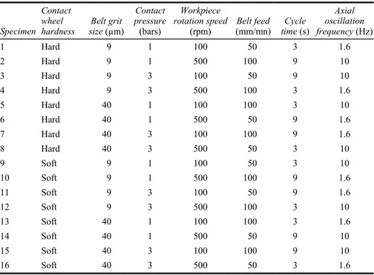
Table 1 Description of the Tagushi experimental design

Specimen

Contact wheel

hardness size (µm)Belt grit

Contact pressure

(bars)

Workpiece rotation speed

(rpm) (mm/mn)Belt feed time (s)Cycle

Axial oscillation frequency (Hz) 1 Hard 9 1 100 50 3 1.6 2 Hard 9 1 500 100 9 10 3 Hard 9 3 100 50 9 10 4 Hard 9 3 500 100 3 1.6 5 Hard 40 1 100 100 3 10 6 Hard 40 1 500 50 9 1.6 7 Hard 40 3 100 100 9 1.6 8 Hard 40 3 500 50 3 10 9 Soft 9 1 100 50 3 10 10 Soft 9 1 500 100 9 1.6 11 Soft 9 3 100 50 9 1.6 12 Soft 9 3 500 100 3 10 13 Soft 40 1 100 100 3 1.6 14 Soft 40 1 500 50 9 10 15 Soft 40 3 100 100 9 10 16 Soft 40 3 500 50 3 1.6

In this experimental design, the following interactions are considered: • contact wheel hardness vs. belt grit size

• contact wheel hardness vs. contact pressure • belt grit size vs. contact pressure.

2.3 Roughness measurements

For all the 16 specimens, 30 roughness profiles were recorded from tooled surfaces by a KLA-TENCORTM _{P-10 profilometer with a 2-µm tip radius. The scanning length} and the sampling length were, respectively, 8 mm and 0.1 µm. Before being treated, all profiles were previously rectified by third degree polynomial fitting.

2.4 Treatments

In the multi-scale approach, each profile is considered at the maximal scanning length that gives relevant correlation between the roughness parameters recorded and a physical process (here the experimental conditions corresponding to the two-level of the experimental design). This approach needs first a local rectification of the profile. Secondly, few roughness parameters are calculated on each part of the profile corresponding to the considered evaluation length. A precedent extensive study on the roughness parameter of machined surface shows that the following parameters are among the more extensively used:

• arithmetic and quadratic roughness (respectively noted, Ra and Rq) • maximal amplitude of profile roughness (noted Rt)

• arithmetic and quadratic means of profile slopes (respectively noted, įa and įq) • arithmetic and quadratic means of profile wavelength (respectively noted, Ȝa and Ȝq) • mean width of profile peaks (noted Sm)

• fractal dimension calculated with the oscillation method (Tricot, 1993).

Next parameters calculation needs to split the profile in five same length sub-profiles. • mean of maximum heights of the five sub-profiles roughness (noted Rpm) • mean of minimum heights of the five sub-profiles roughness (noted Rv) • mean of maximal amplitude of the five sub-profiles roughness (noted Rz).

2.4.1 Local fitting

This fitting aims to erase ‘the local shape’ of the profile at the considered evaluation length. For this purpose, the choice of a first degree B-spline function fitting was made for the reasons developed here as follows.

First degree B-spline functions are described by a series of control points {P0, P1,…, Pk} and a knot sequence {u0, u1,…, uk}. In a parametric description, the

knots values correspond to the parameter u of the B-spline and we have the relation (1).

,1 0 ( ) K i. i ( ) i P u P N u = =

_¦

where Ni,n(u) is a polynomial function with degree n defined by the series (Farin, 1996):

1 , , 1 1, 1 1 1 ( ) ( ) k l n k n k n k n l n l l n l u u u u N N u N u u u u u − + − − − + − − + − − = + − − 1 ,0 1 if [ , ] with ( ) . 0 else i i i u u u N u _{= ®}­ ∈ − ¯

In our case, the u parameter was taken equal to the scanning length X that varies between 0 mm and 8 mm. The fitting consists in finding the ordinate of each control point Pi

which minimises the quadratic distance

¦

profile points. The formalism is the following:

The quadratic distance is minimised by the relation (2)

,1 ,1 0 0 . ( ) ( ) 0 p K i j i i i i j p Pj N x N x = = ª º − = « » ¬ ¼

¦

¦

which corresponds to the following matrix representation:

[

]

_¦

_¦

The series of control points is given by equation (5)

1_{. .}

P M Y₌ −

JG JG

(5) Figure 2 presents an example of profile fitted by a first degree B-spline. The B-spline

function is not derivable at each control point so, consequently the rectified profile loses its C1 _{continuity. For this reason, control points were located at boundaries between} each interval under study corresponding to the evaluation length. In contrast to the technique consisting in making a simple polynomial fitting on each interval under study, this method allows to keep the continuity of the global profile. It induces to consider not only the information contained in the current interval, but also the information contained in the two adjacent intervals. In another way, it is equivalent to take in account the heterogeneity of the shape along the profile during the calculation of local roughness parameters. By ‘shape’, we mean all the information located at a longer wavelength than the evaluation length.

Figure 2 Example of profile fit by a first degree B-spline with 30 control points

(see online version for colours)

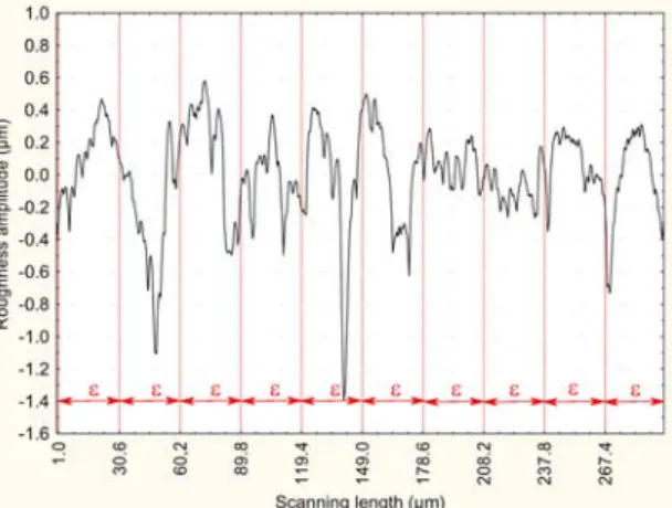
2.4.2 Roughness parameters computation

Each profile is first split into sub-profiles as long as the evaluation length as shown in Figure 3. Next, few current roughness parameters are calculated for each sub-profile. The parameter pε, related to the current evaluation length ε, is defined as the mean value

of the parameter pε,i calculated on the ith sub-profile. This pε value is considered as a

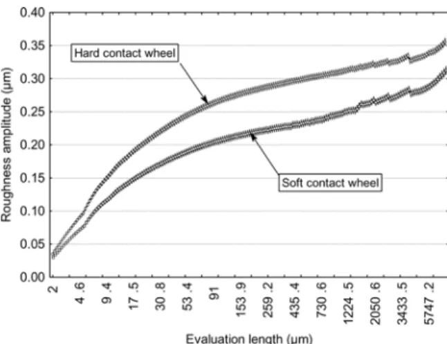
representation of the roughness parameter p along the profile for the evaluation length. In other terms, we consider the profile roughness as ergodic, i.e., the roughness is homogeneous along the profile at the current scale. This point constitutes a difference with regard to the wavelet method because we take in account any information about the roughness location. Rectification and roughness parameters calculation are repeated for a range of evaluation length from the profilometer tip radius (2 µm) to the scanning length (8 mm). The evolution of the arithmetic roughness parameter vs. the evaluation length and the contact wheel hardness is given in Figure 4. Figure 4 shows that the difference between values of arithmetic roughness mean corresponding to each level of contact wheel hardness varies with the evaluation length. The difference vanished at an evaluation length of about 2 µm. This scale corresponds to the tip radius and defines the value under which the recorded profile begins to be smooth. Consequently, lower scales are not relevant.

Figure 4 Evolution of means of arithmetic roughness vs. the evaluation length

for the two levels of contact wheel hardness

The main problem is now to select the most relevant evaluation length giving the highest roughness difference between groups of specimens tooled with the two contact wheel hardness.

2.4.3 The variance analysis (ANOVA)

The most relevant scale is investigated by variance analysis, which is an implementation of the generalised linear model. The formalism is as follows:

Let 1 2 1 2 0 , 1 , , , , , , , 1 1 ( , , , , , ) ( , ) ( , ) ( , ) j j l p p i p j k j p p j k l k k k k n j l j p k k k n i i i ε α α ε β ε ξ ε = = = + = + + +

¦

¦ ¦

the p process parameters are taken at levels k1, k2,…, kp, for an ε evaluation length.

, j( , )

j k i

α ε is the influence on the roughness parameter value of the jth process parameter at kj level and βj k l k, , ,j l( , )i ε is the influence of the interaction between both kj and kl

process parameters. ξk k₁, , ,₂!k np, ( , )i ε is a Gaussian noise with null value and σ standard

deviation.

For each evaluation length, all of these influences are calculated by linear fitting. From them and for each process parameter and each interaction, between-group variability and within-group variability (corresponding to errors of estimation of the roughness parameter into each group) are calculated. The result noted F(pi,ε) is the ratio

produced by dividing the between-group variability by the within-group variability. In other words, this result compares the effect of each process parameter on the roughness parameter value with its estimation error. Consequently, for a given process parameter, a value of F(pi, ε) more than one translates an relevancy of the roughness

parameter pi estimated at the evaluation length ε to represent effects of the considered

at the scale _{ε is (see Benoist et al., 1995 for more details). In this way, we can compare} not only the F(pi,ε) values with regard to the evaluation length but also to the chosen

roughness parameter. By looking for the highest F(pi,ε) value, we can select the most

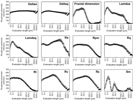
pertinent roughness parameter and its evaluation length to describe the influence of the given process parameter. For the case of the hardness of contact wheel, Figure 5 presents the evolutions of F(pi,ε) vs. the evaluation length for each roughness parameter

calculated.

Figure 5 Evolution of relevancy of each roughness parameter vs. the evaluation length

to put in evidence effects of contact wheel hardness

These graphs show that the range of relevant evaluation lengths depends on the type of roughness parameter. Only hybrid parameters (įa and įq) are relevant at macroscopic scales corresponding to the scanning length (8 mm). Amplitude parameters are the most pertinent at mesoscopic scales (few hundreds of µm) and frequency parameters (Ȝa and Ȝq) at microscopic scale (few µm). One can already conclude that the contact wheel hardness have two effects on amplitude and on frequency of roughness.

3 Results and discussion

3.1 Effect of the contact wheel hardness

Figure 5 shows that the contact wheel hardness influences the amplitude and the frequency parameters at different scales. Evolutions of the most relevant roughness parameter of each type vs. the hardness of contact wheel are given in Figure 6.

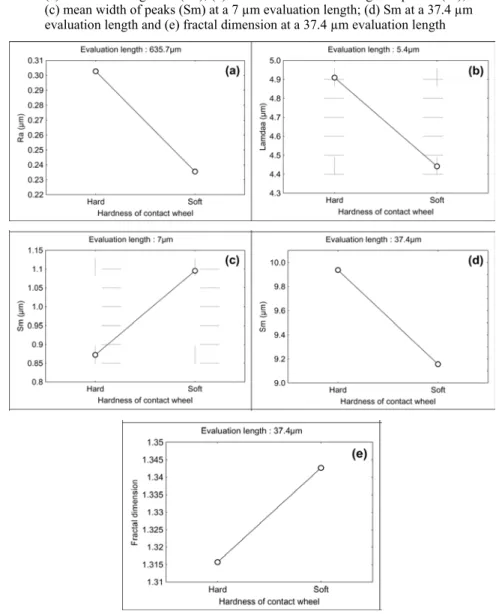
Figure 6 Effects of contact wheel hardness on the most relevant roughness parameters:

(a) arithmetic roughness (Ra); (b) arithmetic mean wavelength of profile (Ȝa); (c) mean width of peaks (Sm) at a 7 µm evaluation length; (d) Sm at a 37.4 µm evaluation length and (e) fractal dimension at a 37.4 µm evaluation length

From these graphs, we can affirm that lower the hardness of contact wheel is: • lower the roughness amplitude is

• lower the mean wavelength is

• lower the mean width of peaks is at a mesoscopic scale but higher it is at a microscopic scale

• higher is the fractal dimension.

These results can be explained by the capacity of the contact wheel to transmit contact pressure to each grain of the belt. Indeed, the soft contact wheel is much able to be deformed by the contact pressure to compensate grain size irregularities

and surface topography. In this case, the pressure distribution on belt surface is more uniform, which induces a decrease of the local maximum pressure acting on the grains and as a consequence a lower penetration in tooled part decreases the roughness amplitude. The mean width of peaks is lower for an evaluation length about the grain size. Globally, the number of working grains rises that induces a more random profile and an increase of the fractal dimension as seen in Figure 7.

Figure 7 SEM of specimens tooled with a hard contact wheel (on the left) and with a soft

contact wheel (on the right) observed at a scale corresponding to the evaluation length of the fractal dimension

At the microscopic scale, the contact wheel hardness modifies the mean width of peaks (Sm) differently with regards to the macroscopic scale. The soft contact wheel deformation induce the belt’s one and the bottom of grooves can be tooled whether for high hardness, only the top of roughness is in contact with the belt. As a result, the mean wavelength is shorter as seen in Figure 8.

Figure 8 SEM of specimens tooled with a hard contact wheel (on the left) and with a soft

contact wheel (on the right) observed at the microscopic influence scale

3.2 Effect of the belt grit size

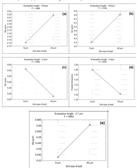
The method developed in the preceding section is now used to study the belt grit size effect. The results are shown in Figure 9, which represents different roughness parameters calculated at an evaluation length for which difference between the two grit sizes is maximum. Higher the grit size is, higher the arithmetic roughness is Figure 9(a). Moreover, the peaks mean width presents two relevant evaluation lengths: 3.7 µm and 19.5 µm. These scales might correspond to the mean width of scratches induced

by each grit size. This aspect can be modelled as follows: At a 19.5 µm evaluation length, both sizes of scratches can be observed and the peaks mean width is higher for specimens tooled with a 40-µm grit size (Figure 9(b)). Under this evaluation length, peaks of profiles extracted from 40-µm grit size machined surfaces are more and more filtered by the local fitting. As a consequence, at the 3.7-µm evaluation length, asperities of workpiece tooled with a 9-µm grit size are preserved, while using a 40-µm grit size profiles show only micro-scratches in the groves (Figures 10 and 11). With a 9-µm grit size, the fractal dimension is higher, and the mean width of peaks is twice the value recorded for 40-µm grit size condition (Figure 9(c) and (d)). This result is confirmed by scanning electron microscopy in Figure 11. This micro-roughness gives a less random aspect to the profile, which decreases the fractal dimension and increases the arithmetic roughness (Figure 9(e)).

Figure 9 Effects of belt grit size on the most relevant roughness parameters:

(a) arithmetic roughness at an evaluation length of 19.5 µm; (b) mean width of peaks at the same scale; (c) mean width of peaks at 3.7 µm; (d) fractal dimension at 3.5 µm and (e) arithmetic roughness at 2.7 µm

Figure 10 Model of effects of evaluation length on the roughness evolution vs. the belt grit size

(see online version for colours)

Figure 11 SEM of grit size effects (9 µm on the left and 40 µm on the right) on roughness

at microscopic scale

3.3 Effect of contact pressure

Figure 12 shows that higher the contact pressure is, higher is the mean width of peaks at a large evaluation length and lower it is at a microscopic scale. These effects might be interpreted like the ones of the contact wheel hardness. Indeed, higher the contact pressure, higher the grains penetration that increases the peaks width at large scale. From a microscopic point of view, pressure leads to damage tooling conditions. Indeed, instead of being ‘cut’ by the belt grains, the material is moved to fill the scratches as shown in Figure 13 and resulting peaks mean width is then lower.

Figure 12 Effects of contact pressure on the peaks mean width: Sm relevancy vs. the evaluation

Figure 13 SEM of effect of wrong cutting conditions induced by high contact pressure

(on the right) with regards to low contact pressure (on the left)

3.4 Influence of workpiece rotation speed and cycle time

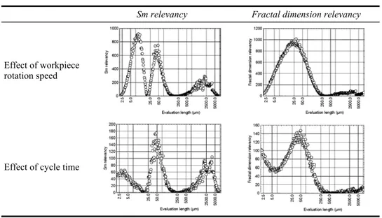
These process parameters have been studied together because of their similar effects as shown in Table 2. Indeed, we observe that both of these process parameters have an effect on Sm and the fractal dimension quite at the same evaluation length (47.1 µm for Sm and 40 µm ± 10 µm for the fractal dimension). Evolution graphs of these parameters are given in Table 3. Table 3 shows that higher the rotation speed or the cycle time is, lower the peaks mean width is and higher the fractal dimension is. In fact, in each case, the number of cut increases, which induce a more uniform roughness (see Figure 14). The surface seems to be random, the Sm decreases and the fractal dimension rises. In Table 2, the Sm relevancy curve relative to the rotation speed presents a second peak of pertinence for a 9.4 µm evaluation length. The evolution of this parameter at this scale is given in Figure 15. Figure 15 shows that Sm increases at a 9.4-µm evaluation length when rotation speed rises. Presumably, that can be explained by wrong ‘cutting’ conditions. With low-rotation speed, the materials have a tendency of being pushed instead of being cut and fill the scratches as shown in Figure 16. Rotation speed has the same effect as the contact pressure.

Table 2 Comparison of workpiece rotation speed and cycle time effects on the most relevant roughness parameters

Sm relevancy Fractal dimension relevancy

Effect of workpiece rotation speed

Table 3 Evolutions of each relevant roughness parameter vs. the workpiece rotation speed and cycle time

Effect on Sm Effect on the fractal dimension

Effect of the workpiece rotation speed

Effect of cycle time

Figure 14 SEM of rotation speed effect (100 rpm on the left and 500 rpm on the right)

and cycle time (3 s on the left and 9 s on the right). Magnitude corresponds to the evaluation length

Figure 16 SEM of effect of wrong cutting conditions induce by low rotation speed

3.5 Effects of other process parameters

The results obtained for the belt feed and the axial oscillation frequency are shown, respectively, in Figures 17 and 18. It can be observed that pertinent roughness parameters are relevant at the minimum scale corresponding to the tip radius of the profilometer. To explain this result, a study should be done at lower scales with an AFM for example.

Figure 17 Relevancy of roughness parameters vs. the evaluation length to describe

Figure 18 Relevancy of roughness parameters vs. the evaluation length to describe

effects of the axial oscillation frequency

3.6 Effect of interactions

For the same reasons, only the interaction between belt grit size and contact pressure can be explained. The effects are plotted in Figure 19. This result can be explained as follows:

• For a low contact pressure, the surface tooled with low grit size has a lower mean 4 peaks width as seen before. It induces that, at a 23.8-µm evaluation length, this surface looks like random and the fractal dimension is higher: in other terms, grid size effect is dominant.

• For high contact pressure and a large grit size, the increase in the fractal dimension observed in Figure 19 could be explained by the apparition of ductile ploughing as seen in Figure 20. Yet, this result must be confirmed by a more precise study.

Figure 20 SEM of ductile ploughing observed on specimen n°8 (high contact pressure

and high grit size)

4 Conclusion

This paper outlines a multi-scale method for roughness measurements to put in evidence the effects of the working conditions in the belt grinding process on the surface topography.

Most of the seven retained process parameters have an influence on roughness, in particular, on the mean width of peaks (Sm). The most relevant evaluation length of roughness parameters depends both on the roughness parameter and on the belt grinding process parameter under consideration. As a consequence, it is important to select the best scale to study each physical phenomenon.

Results have shown that effects currently explained in the bibliography were confirmed for the macroscopic scale. Other roughness parameters will be implemented in our analysis system to better characterise surfaces at different scales. Another improvement could be to give the confidence interval of the F value by using a bootstrap protocol.

References

Axinte, D.A., Kritmanorot, M., Axinte, M. and Gindy, N.N.Z. (2005) ‘Investigations on belt polishing of heat-resistant titanium alloys’, Journal of Materials Processing Technology, Vol. 166, pp.398–404.

Benoist, D., Tourbier, Y. and Germain-Tourbier, S. (1995) Plans d’expériences – construction et

analyse, Tec and Doc., January, Paris.

Farin, G. (1996) Curves and Surfaces for Computer-Aided Geometric Design – A Practical Guide, 4th ed., Academic Press, New York.

Ghidossi, P., El Mansori, M., Sura, E., Geoffroy, R. and Deblaise, S. (2005) ‘Procédé de superfinition par toilage: analyse énergétique des variables process – temps de cycle et fréquence d’oscillation’, Integrated Design and Production – 4th International Conference, Casablanca, Maroc, November, paper 101 – theme 13.

Huang, H., Gong, Z.M., Chen, X.Q. and Zhou, L. (2002) ‘Robotic grinding and polishing for turbine-vane overhaul’, Journal of Material Processing Technology, Vol. 127, pp.140–145. Jourani, A., Dursapt, M., Hamdi, H., Rech, J. and Zahouani, H. (2005) ‘Effect of the belt grinding

Khellouki, A., Maiz, H., Rech, J. and Zahouani, H. (2005) ‘Application de la méthode des plans d’expériences à la caractérisation du procédé de toilage de superfinition’, Integrated

Design and Production – 4th International Conference, Casablanca, Maroc, November,

paper 95 – theme 2.

Rech, J. and Moisan, A. (2003) ‘Le toilage: un moyen d’optimisation de l’intégrité des surfaces usinées’, 16ème _{congrès Français de Mécanique, Nice, France, September.}

Tricot, C. (1993) courbe et dimension fractale, Spinger-Verlag, Paris.

Zhang, X., Kuhlenkötter, B. and Kneupner, K. (2005) ‘An efficient method for solving the Signorini problem in the simulation of free-form surfaces produced by belt grinding’,