Advances in deep learning with limited supervision and computational resources
Texte intégral
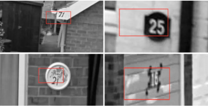
Figure

Documents relatifs
As a remedy to such problem, we propose to use the generative models which were proposed by Ian Goodfellow and al in [1] providing the AI world with a new class of Deep Learning
A week after the submission of the final project, the students were asked to fill in a questionnaire, and 18 students responded. We asked about programming experience and what
a flat collection of binary features resulting from multiple one-hot-encodings, discarding useful information about the structure of the data. To the extent of our knowledge, this
We presented the VS task for refining the final grasping pose prior to grasp to address the challenges linked to final gripper pose, reported in literature related to transfer
We then present its fully- convolutional variation, Spatial Generative Adversarial Networks, which is more adapted to the task of ergodic image generation.. 2.1 Generative
However, in the domain of materials science, there is a need to synthesize data with higher order complexity compared to observed samples, and the state-of-the-art cross-domain GANs
Our work falls into the category of text to image CGANs [13, 16], where we explore the possibility of obtaining good multimodal representations from the discriminator, while using
Our goal is similar (reproducing pedestrian motion at the full trajectory level), but our approach is different: we learn the spatial and temporal properties of complete
