RefPlanets: Search for reflected light from extra-solar planets with SPHERE/ZIMPOL
Texte intégral
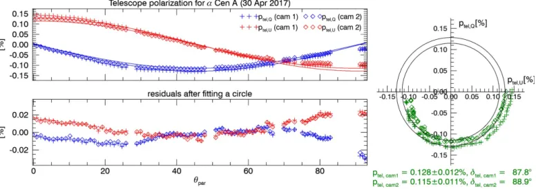
Figure

Documents relatifs
With two pairs of planets with a period ratio lower than 1.5, with short orbital periods, low masses, and low eccentricities, HD 215152 is similar to the very compact
Cet article présente les préliminaires d’un modèle de perception multi-sens, Présence, qui définit une architecture modulaire et générique pour permettre à des agents évoluant
Join, A multicentury stable isotope record from a New Caledonia coral: Interannual and decadal sea surface temperature variability in the southwest Pacific since 1657
Jean-Marie Saurel, Claudio Satriano, Constanza Pardo, Arnaud Lemarchand, Valérie Clouard, Céline Dessert, Aline Peltier, Anne Le Friant,..
We propose that slow slip events are ductile processes related to transient strain localisation, while non-volcanic tremor correspond to fracturing of the whole rock at
• Photometric and spectrometric combination method (as in Bovy et al. [ 2014 ]): it is based on the selection of RC stars by their position in a colour - metallicity - surface
Two capillary pressure and two relative permeability experiments were performed, enabling these properties to be determined for two sets of pressures and
Discussion: With N = 2, either type of investor (risk-neutral or risk-averse) has an incentive to plunge into dependence if there is enough geological dependence among
