Letter
https://doi.org/10.1038/s41586-019-1550-3Rapid expansion of Greenland’s low-permeability
ice slabs
M. MacFerrin1*, H. Machguth2,3, D. van As4, C. Charalampidis5, C. M. Stevens6, A. Heilig7,8,9, B. Vandecrux4,10, P. L. Langen11,
r. Mottram11, X. Fettweis12, M. r. van den Broeke13, W. t. Pfeffer14, M. S. Moussavi1,15 & W. Abdalati1 In recent decades, meltwater runoff has accelerated to become the
dominant mechanism for mass loss in the Greenland ice sheet1–3. In Greenland’s high-elevation interior, porous snow and firn accumulate; these can absorb surface meltwater and inhibit runoff4, but this buffering effect is limited if enough water refreezes near the surface to restrict percolation5,6. However, the influence of refreezing on runoff from Greenland remains largely unquantified. Here we use firn cores, radar observations and regional climate models to show that recent increases in meltwater have resulted in the formation of metres-thick, low-permeability ‘ice slabs’ that have expanded the Greenland ice sheet’s total runoff area by 26 ± 3 per cent since 2001. Although runoff from the top of ice slabs has added less than one millimetre to global sea-level rise so far, this contribution will grow substantially as ice slabs expand inland in a warming climate. Runoff over ice slabs is set to contribute 7 to 33 millimetres and 17 to 74 millimetres to global sea-level rise by 2100 under moderate- and high-emissions scenarios, respectively— approximately double the estimated runoff from Greenland’s high-elevation interior, as predicted by surface mass balance models without ice slabs. Ice slabs will have an important role in enhancing surface meltwater feedback processes, fundamentally altering the ice sheet’s present and future hydrology.
A field campaign carried out in spring 2012 at the KAN_U field site at 1,840 m above sea level (a.s.l.) in southwest Greenland’s accu-mulation area found 3–5-m-thick layers of refrozen meltwater in firn cores just below the seasonal snow layer5,6. The record-breaking 2012
Greenland summer melt7,8 caused meltwater to visibly run off from
KAN_U over the top of these layers for the first time on record instead of refreezing locally in porous firn. Thick ice layers resulted in approx-imately 11 ± 3% more runoff in that region than would have occurred without the blocking effect of subsurface ice5.
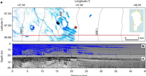
The Spring 2013 Arctic Circle Traverse (ACT-13) campaign in south-west Greenland mapped a continuous 40-km-long, multimetre-thick ice slab along an uphill transect in southwest Greenland (Fig. 1). Runoff was routed over the top of this slab instead of being fully absorbed into the firn column. During the 2012 summer, the equilibrium line altitude, where annual melt equals accumulation, was estimated to be approximately 1,900 m a.s.l.
In this work we distinguish between ice lenses and ice slabs in firn. Ice lenses are thin (0–10 cm) refrozen ice layers that form in a single melt season in the percolation area of the ice sheet9,10. Meltwater can
percolate through and around lenses11 along preferential flow paths,
sometimes reaching depths of 10 m or more before refreezing12. Layers
of refrozen ice between 10 cm and 1 m thick—primarily multi-annual refreezing features—were documented in 201611 in cores and deep pits
in southwest Greenland’s percolation area up to an altitude of 2,100 m
a.s.l., but their horizontal extent appeared limited and not able to cause runoff over wide areas. Low-permeability ice slabs are thicker refrozen layers (≥1 m thick) that form when water refreezes between preexisting ice layers, annealing them together. Slabs form over multiple years, can span horizontally for tens of kilometres and cause the permeability of the near-surface firn layer to approach zero13 despite pore space
avail-ability at greater depth. Ice slabs are spatially continuous enough to be mapped over great distances by ground-penetrating radar surveys. Here we focus solely on ice slabs in Greenland’s firn that block deep percolation and enhance runoff.
We present an observational map of ice slabs across the Greenland ice sheet, created from surveys performed by ground-penetrating radar (GPR) and NASA’s IceBridge airborne Accumulation Radar (IceBridge AR), and validated against firn cores drilled along the GPR surveys. We use an empirical model to quantify the present-day formation of ice slabs from the outputs of regional climate models (RCMs). Using RCMs forced on their boundaries by forward-looking general circula-tion models (GCMs), we forecast the growth of ice slabs and their con-tributions to runoff under the Representative Concentration Pathway (RCP) 4.5 and 8.5 (moderate- and high-emissions, respectively) sce-narios through the end of the 21st century.
Shallow firn cores retrieved along the ACT-13 transect contain ≥1-m-thick ice slabs at sites below 2,000 m a.s.l. (Extended Data Fig. 1a, cores 1–3, and Extended Data Fig. 2)5. Ice slabs at KAN_U
have grown progressively thicker; in five years, the ice volume content of the top 10 m grew from 54% in 2012 to 73% in 2017 (Extended Data Fig. 1b), with nearby locations experiencing similar growth (Extended Data Fig. 1c).
In situ GPR measurements show ice slabs beginning at approxi-mately 1,700 m a.s.l. along the ACT-13 transect (Fig. 1b), indicating that in 2012 the long-term runoff limit had migrated up to the KAN_U site at 1,840 m a.s.l., consistent with satellite observations5. Ice slabs
detected from a spatially coincident transect of IceBridge AR, flown three weeks before the ACT-13 transect, closely match results in the top 20 m of firn with a vertical error of −21% to +6% compared to adjacent cores, partially underestimating the ice volume but accurately measuring the overall extent of ice slabs within the top 20 m of firn. A survey of IceBridge AR flight lines from 2010–2014 (Fig. 2) show that ice slabs covered 64,800–69,400 km2 of the Greenland ice sheet in 2014,
or approximately 4% of the ice sheet’s total area. We identify ice slabs as continuous layers of near-surface ice above porous layers of firn; they have a thickness of 1–16 m in the top 20 m of firn and extend contin-uously for ≥1 km along an IceBridge flight line. We adjust the thick-ness observations of IceBridge AR according to the range of thickthick-ness uncertainties, map spatially continuous slabs of 1–16 m thickness and interpolate polygons around continuous areas of ice slabs to estimate 1Cooperative Institute for Research in Environmental Sciences, University of Colorado, Boulder, CO, USA. 2Department of Geosciences, University of Fribourg, Fribourg, Switzerland. 3Department
of Geography, University of Zurich, Zurich, Switzerland. 4Geological Survey of Denmark and Greenland, Copenhagen, Denmark. 5Bavarian Academy of Sciences and Humanities, Munich, Germany. 6Department of Earth and Space Sciences, University of Washington, Seattle, WA, USA. 7WSL Institute for Snow and Avalanche Research SLF, Davos Dorf, Switzerland. 8Department of Earth
and Environmental Sciences, Ludwig-Maximilians-University of Munich, Munich, Germany. 9Alfred Wegener Institute Helmholtz-Centre for Polar and Marine Research, Bremerhaven, Germany. 10Department of Civil Engineering, Technical University of Denmark, Kongens Lyngby, Denmark. 11Danish Meteorological Institute, Copenhagen, Denmark. 12Department of Geography, University
of Liège, Liège, Belgium. 13Institute for Marine and Atmospheric Research, Utrecht University, Utrecht, The Netherlands. 14Department of Civil Engineering, University of Colorado, Boulder, CO,
USA. 15National Snow and Ice Data Center, University of Colorado, Boulder, CO, USA. *e-mail: michael.macferrin@colorado.edu
their area. Potential gaps in airborne data coverage make this range a conservative estimate of the total extent of ice slabs in Greenland.
RCMs forced at their boundaries by atmospheric reanalysis data (see Methods) at the locations where IceBridge AR has observed ice
slabs suggest that ice slabs occur where annual snow accumulation is below 572 ± 32 mm water equivalent (w.e.). Ice slabs appear to be absent in regions of high accumulation in which surface meltwater is trapped in perennial firn aquifers instead of refreezing14,15; this is
1,900 1,800 1,700 67.04 67.00 66.96 –47.50 –47.00 –46.50 0 5 km a 0 10 20 10 20 0 5 10 15 20 25 30 35 40 45 Distance (km) Longitude (°) Depth (m) Latitude (°) b c
Fig. 1 | Meltwater runoff over low-permeability ice slabs in southwest Greenland. a, ACT-13 transect path (red line) overlaid on a LandSat-7
image from 16 July 2012 (contrast-enhanced to show surface water in blue). KAN_U is noted with the red star. 50-m contours from the Arctic Digital Elevation Model (ArcticDEM release 7)31 are shown, and elevations
are in metres above sea level. b, Data obtained with 800-MHz GPR during the ACT-13 campaign, showing depths of 0–20 m. Layers of refrozen ice are coloured blue. c, Data from a 2013 transect of 550–900 MHz IceBridge AR over the same line, showing depths of 0–20 m.
80 70 60 –80 –70 –60 –50 –40 –30 –20 –10 0 1–4 4–7 7–10 10–13 13–16 Ice-slab thickness (m) 0 400 km 0 40 km 0 40 km a b c b c Longitude (°) Latitude (° )
Fig. 2 | Low-permeability ice slabs on the Greenland ice sheet and peripheral ice caps detected by IceBridge AR (2010–2014). a–c, Ice slabs detected
in Greenland with −21% to +6% thickness uncertainty. b, c, Zoom-ins (6×) on northeast (b) and southwest (c) Greenland.
consistent with firn models showing aquifers that form in regions with annual accumulation rates exceeding about 600 mm w.e.16.
RCMs forced at their boundaries by atmospheric reanalysis data show that ice slabs have formed in regions receiving 266–573 mm w.e. yr−1
excess melt for a decade or more (Supplementary Information Fig. 16). Here, ‘excess melt’ refers to the amount of meltwater beyond the capacity of annual accumulation to absorb and refreeze it, result-ing in excess water, which fills surroundresult-ing firn layers or runs off to lower elevations (see Methods). In ten years, the upper value of that range (573 mm w.e. yr−1) would transform a shallow porous firn layer
(density of 450–550 kg m−3) into refrozen ice with bubbles (density
of 873 kg m−3) to a thickness of 13.6–17.7 m, in agreement with the
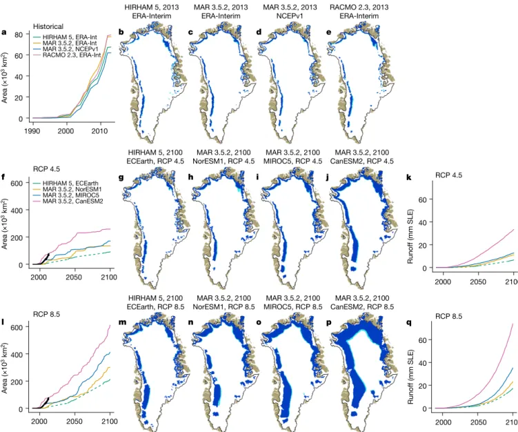
maximum-thickness threshold of 16 m used when detecting ice slabs with IceBridge AR. RCMs show that in data pixels containing ice slabs detected by IceBridge AR, excess melt increased slowly since the 1990s (Extended Data Fig. 3) and then rapidly after 2001, causing the inferred annual rates of ice slab formation to increase ten times or more (Table 1, Fig. 3a). At the end of 2013, RCMs estimate that ice slabs in Greenland covered an area 62,100–78,900 km2 larger than Greenland’s pre-1990
runoff area. Maps of simulated ice slabs at the end of 2013 (Fig. 3b–e) are consistent with one another, as well as with the extent observed by IceBridge AR (Fig. 2). Within individual ice-sheet drainage basins, simulated ice slab elevations match within uncertainties in nearly every case (Extended Data Fig. 4). Inconsistencies between observed and simulated ice slabs exist primarily in east and southeast Greenland, where ice slabs are limited to relatively small and isolated areas that are difficult to cover fully by airborne IceBridge AR campaigns.
RCMs forced by GCMs until 2100 show that the area of ice slabs across Greenland is likely to expand moderately through 2050 under both RCP 4.5 (Fig. 3f) and RCP 8.5 (Fig. 3l) forcing, approximately doubling in area compared to its present extent. Models forced by RCP 4.5 show a relative slowdown of growth in ice-slab extent after 2050 through 2100 (Fig. 3f). Most ice-slab simulations forced by GCMs underestimate the current extent of ice slabs when compared to rea-nalysis-forced RCMs (Fig. 3a), in part because present-day GCMs do not capture atmospheric circulation changes over Greenland that have contributed to recent summer melt increases17. Under the RCP 8.5
scenario, the formation of new ice slabs accelerates from their 1990– 2050 growth (1,240–4,160 km2 yr−1) to approximately double that rate
(2,890–7,130 km2 yr−1) in the latter half of the century (Fig. 3l, Table 1).
In all cases, trends before and after 2050 are statistically significant (P < 0.02).
In 1990–2100, ice slabs are expected to cover 2.3 times larger area and cause 2.4 times more surface runoff, on average, under the RCP 8.5 pathway than under RCP 4.5. Once ice slabs have formed, runoff is cal-culated as the amount of melt that exceeds the near-surface pore space and the cold content that have accumulated since the ice slabs initially formed (see Methods). Without explicitly handling the effects of ice slabs, by 2100 RCMs underestimate the cumulative runoff from areas that are above the pre-1990 runoff area by an average of 56% under RCP 4.5 and 42% under RCP 8.5, compared to equivalent estimates including ice slabs. In both scenarios, this implies a near-doubling of runoff from the interior of the ice sheet due to rapidly decreased surface porosity.
Polar firn is sensitive to relatively small changes in annual meltwa-ter production18,19, and the addition of large areas of new ice slabs in
Greenland is indicative of a departure from steady-state climate that amplifies several types of positive-mass-loss feedback. For instance, meltwater saturation of the ice-sheet surface at KAN_U in 2012 resulted in 9% lower summer albedo and the absorption of 28% additional solar radiation, of which 71% was translated into melt20. This melt–albedo
feedback is not fully captured in the RCMs presented here, so future meltwater estimates may be underestimated. Under linear warming conditions, linear changes in runoff elevation cover increasingly larger areas of the ice sheet’s flat interior6, resulting in parabolic increases in
runoff area (parabolic fit with a power of ~2.5 with respect to elevation) and runoff volume (power of ~3.5)21.
Surface features such as firn cracks, supraglacial streams, lakes and moulins are important components of the ice sheet’s hydrological net-work22. The amount of recent meltwater in Greenland has been
unprec-edented over the past several centuries23 and is expected to keep rising
in a warming climate, forming supraglacial lakes and other features progressively higher on the ice sheet24. It is uncertain whether such
features at high elevations could facilitate water reaching the engla-cial or subglaengla-cial system25, which is a necessary condition for dynamic
feedback processes such as cryo-hydrologic warming26 or meltwater
reaching previously frozen regions of the ice-sheet bed27. However,
recent observations of ice motion at KAN_U show accelerated flow in
Table 1 | RCM results for ice-slab growth and runoff
RCM, forcing Area trend (km2 yr−1) Total area (km2) Runoff trend (Gt yr−1) Runoff acceleration (Gt yr−2) (Gt)Total runoff Area trend (km2 yr−1) Total area (km2) Runoff trend (Gt yr−1) Runoff acceleration (Gt yr−2) Total runoff (Gt)
Historical 1990–2000 2000 1990–2000 1990–2000 2000 2001–2013 2013 2001–2013 2001–2013 2013 HIRHAM 5, ERA-Int. 234 2,500 0.099 0.055 1.42 5,540 67,500 13.7 2.28 166 MAR 3.5.2, ERA-Int. 148 1,410 0.079 0.040 1.07 6,510 77,300 18.5 3.19 222 MAR 3.5.2, NCEP v1 53.3 491 0.025 0.013 0.35 5,300 62,100 12.5 2.48 153 RACMO 2.3, ERA-Int. 330 3,310 0.209 0.070 2.35 6,310 78,900 16.2 2.74 200 21st century RCP 4.5 1990–2050 2050 1990–2050 1990–2050 2050 2051–2100 2100 2051–2100 2051–2100 2100 HIRHAM 5, ECEartha 1,080 53,500 9.67 0.556 514 817 91,700 34.9 0.531 2,380 MAR 3.5.2, NorESM 1 1,280 85,400 11.9 0.698 822 945 135,000 66.4 0.432 3,970 MAR 3.5.2, MIROC 5 1,980 108,000 21.6 0.957 1,330 1200 170,000 66.0 0.834 4,570 MAR 3.5.2, CanESM 2 3,520 205,000 59.5 2.51 3,660 762 258,000 166 1.03 12,000 RACMO 2.1, HadGEM 2b3,970 216,000 46.5 1.96 2,810 3,095 344,000 172 2.35 11,000 21st century RCP 8.5 1990–2050 2050 1990–2050 1990–2050 2050 2051–2100 2100 2051–2100 2051–2100 2100 HIRHAM5, ECEartha 1,240 62,900 13.4 0.672 682 2,890 212,000 95.6 2.97 6,170 MAR 3.5.2, NorESM 1 1,780 85,500 16.6 0.787 1,010 4,740 301,000 143 5.34 8,300 MAR 3.5.2, MIROC 5 1,610 97,900 17.9 0.842 1,150 6,220 410,000 229 7.48 12,700 MAR 3.5.2, CanESM 2 4,160 243,000 67.3 3.13 4,250 7,130 610,000 440 12.9 26,600
Historical results from 1990–2013; 21st century results from 1990–2100.
aHIRHAM 5 21st-century model results only available in three periods: 2000–2010, 2040–2050 and 2090–2100. The 1900–2050 results are computed using 2000–2010 and 2040–2050 combined
data with gaps interpolated. The 2051–2100 results are computed using 2041–2050 and 2090–2100 combined data.
bRACMO 2.1 21st-century model results conclude in 2098. The 2051–2100 results are computed from 2051–2098 data. RACMO 2.1 results are only available for RCP 4.5, which are included here but
not in the moderate-versus-high-emissions visual comparison in Fig. 3.
2009–2013 and seasonal accelerations that were previously unseen at that elevation28. Although the exact mechanisms of such dynamic
feed-back processes are beyond the scope of this paper, they are consistent with meltwater saturation at the same locations and suggest that one or more meltwater-dynamic feedback processes may already influence dynamic flow at the current locations of ice slabs. Further research is needed to explore the feedback between the hydrologic and dynamic systems of the Greenland ice sheet at high elevations.
Once ice slabs have formed, they need relatively small amounts of meltwater to sustain themselves. Following the extraordinary melt years of 2010 and 2012 in southwest Greenland, melt was more moderate in 2013–2017 (ref. 29), although still greater than the 1949–2017 average30.
Ice slabs continued to grow in thickness in 2013–2017, with new ice freezing atop them, and little to no pore space added to the firn column (Extended Data Fig. 1b). Once low-permeability ice slabs have formed, the only known effective mechanism to eliminate their impact on sat-uration and runoff is a prolonged period of cooler climate or higher snow accumulation that would allow pore space to reaccumulate at the surface19. The fact that ice slabs have continued to thicken and remain
close to the surface once they have formed leaves these areas highly vulnerable to enhanced runoff in subsequent warm summers. In a pro-gressively warming Arctic, ice slabs in Greenland’s interior are poised to become increasingly widespread persistent features, with far-reaching consequences for ice-sheet hydrology, runoff and sea level rise.
Online content
Any methods, additional references, Nature Research reporting summaries, source data, extended data, supplementary information, acknowledgements, peer review information; details of author contributions and competing interests; and state-ments of data and code availability are available at https://doi.org/10.1038/s41586-019-1550-3.
Received: 12 October 2018; Accepted: 8 July 2019; Published online 18 September 2019.
1. van den Broeke, M. R. et al. On the recent contribution of the Greenland ice sheet to sea level change. Cryosphere 10, 1933–1946 (2016).
2. Fettweis, X. et al. Reconstructions of the 1900–2015 Greenland ice sheet surface mass balance using the regional climate MAR model. Cryosphere 11, 1015–1033 (2017). Historical HIRHAM 5, 2013 ERA-Interim MAR 3.5.2, 2013 ERA-Interim MAR 3.5.2, 2013 NCEPv1 RACMO 2.3, 2013 ERA-Interim RCP 4.5 HIRHAM 5, 2100
ECEarth, RCP 4.5 NorESM1, RCP 4.5MAR 3.5.2, 2100 MIROC5, RCP 4.5MAR 3.5.2, 2100
2000 2050 2100 0 20 40 60 Runoff (mm SLE) MAR 3.5.2, 2100 CanESM2, RCP 4.5 RCP 4.5 2000 2050 2100 0 20 40 60 Runoff (mm SLE) RCP 8.5 HIRHAM 5, 2100
ECEarth, RCP 8.5 NorESM1, RCP 8.5MAR 3.5.2, 2100 MIROC5, RCP 8.5MAR 3.5.2, 2100 CanESM2, RCP 8.5MAR 3.5.2, 2100
RCP 8.5 a b c d e f g h i j k l m n o p q 1990 2000 2010 0 20 40 60 80 Area (×10 3 km 2) HIRHAM 5, ERA-Int MAR 3.5.2, ERA-Int MAR 3.5.2, NCEPv1 RACMO 2.3, ERA-Int 2000 2050 2100 0 200 400 600 Area (×1 0 3 km 2) HIRHAM 5, ECEarth MAR 3.5.2, NorESM1 MAR 3.5.2, MIROC5 MAR 3.5.2, CanESM2 2000 2050 2100 0 200 400 600 Area (×1 0 3 km 2)
Fig. 3 | Ice-slab growth and runoff computed by outputs from RCMs.
a–e, RCMs forced by reanalysis datasets (see key in a) through 2013, directly comparable to the ice-slab observations shown in Fig. 2. f–q, 21st-century RCM results forced by GCMs (see key in f) under the RCP 4.5 (f–k) and 8.5 (l–q) pathways. The black line in f and l represents the historical ice-slab growth from a for comparison. Runoff estimates in
k and q show 21st-century runoff in global sea-level-equivalent (SLE)
from the top of ice-slab regions and do not include contributions from Greenland’s historical runoff area. In the maps (b–e, g–j, m–p), headings indicate the RCM, year, reanalysis or GCM boundary dataset, and (for the future projections in g–j and m–p) the RCP pathway. Dark blue areas are continuous ice slabs that can affect runoff and light blue are intermittent ice slabs that do not yet cause runoff. Only continuous ice slabs (dark blue) are included in trend lines.
3. Mottram, R. et al. An integrated view of Greenland ice sheet mass changes based on models and satellite observations. Remote Sens. 11, 1407 (2019). 4. Harper, J., Humphrey, N., Pfeffer, W. T., Brown, J. & Fettweis, X. Greenland
ice-sheet contribution to sea-level rise buffered by meltwater storage in firn.
Nature 491, 240–243 (2012).
5. Machguth, H. et al. Greenland meltwater storage in firn limited by near-surface ice formation. Nat. Clim. Chang. 6, 390–393 (2016).
6. Mikkelsen, A. B. et al. Extraordinary runoff from the Greenland ice sheet in 2012 amplified by hypsometry and depleted firn retention. Cryosphere 10, 1147–1159 (2016).
7. Nghiem, S. V. et al. The extreme melt across the Greenland ice sheet in 2012.
Geophys. Res. Lett. 39, L20502 (2012).
8. Tedesco, M. et al. Evidence and analysis of 2012 Greenland records from spaceborne observations, a regional climate model and reanalysis data.
Cryosphere 7, 615–630 (2013).
9. Benson, C. S. Stratigraphic Studies in the Snow and Firn of the Greenland Ice
Sheet. Research Report No. 70 (US Army Snow, Ice and Permafrost Research
Establishment, 1962).
10. Brown, J., Harper, J., Pfeffer, W. T., Humphrey, N. & Bradford, J. High-resolution study of layering within the percolation and soaked facies of the Greenland ice sheet. Ann. Glaciol. 52, 35–42 (2011).
11. Heilig, A., Eisen, O., MacFerrin, M., Tedesco, M. & Fettweis, X. Seasonal monitoring of melt and accumulation within the deep percolation zone of the Greenland Ice Sheet and comparison with simulations of regional climate modeling. Cryosphere 12, 1851–1866 (2018).
12. Humphrey, N. F., Harper, J. T. & Pfeffer, W. T. Thermal tracking of meltwater retention in Greenland’s accumulation area. J. Geophys. Res. 117, F01010 (2012). 13. Sommers, A. N. et al. Inferring firn permeability from pneumatic testing: a case
study on the Greenland ice sheet. Front. Earth Sci. 5, 20 (2017). 14. Forster, R. R. et al. Extensive liquid meltwater storage in firn within the
Greenland ice sheet. Nat. Geosci. 7, 95–98 (2014).
15. Miège, C. et al. Spatial extent and temporal variability of Greenland firn aquifers detected by ground and airborne radars. JGR Earth Surf. 121, 2381–2398 (2016). 16. Munneke, P. K. M., Ligtenberg, S. R., van den Broeke, M. R., van Angelen, J. H. &
Forster, R. R. Explaining the presence of perennial liquid water bodies in the firn of the Greenland Ice Sheet. Geophys. Res. Lett. 41, 476–483 (2014).
17. Hanna, E., Fettweis, X. & Hall, R. J. Recent changes in summer Greenland blocking captured by none of the CMIP5 models. Cryosphere 12, 3287–3292 (2018).
18. Pfeffer, W. T., Meier, M. F. & Illangasekare, T. H. Retention of Greenland runoff by refreezing: implications for projected future sea level change. J. Geophys. Res.
96, 22117–22124 (1991).
19. Braithwaite, R. J., Laternser, M. & Pfeffer, W. T. Variations of near-surface firn density in the lower accumulation area of the Greenland ice sheet, Pâkitsoq, West Greenland. J. Glaciol. 40, 477–485 (1994).
20. Charalampidis, C. et al. Changing surface–atmosphere energy exchange and refreezing capacity of the lower accumulation area, West Greenland. Cryosphere
9, 2163–2181 (2015).
21. van As, D. et al. Hypsometric amplification and routing moderation of Greenland ice sheet meltwater release. Cryosphere 11, 1371–1386 (2017). 22. Rennermalm, A. K. et al. Evidence of meltwater retention within the Greenland
ice sheet. Cryosphere 7, 1433–1445 (2013).
23. Trusel, L. D. et al. Nonlinear rise in Greenland runoff in response to post-industrial Arctic warming. Nature 564, 104–108 (2018).
24. Fitzpatrick, A. A. W. et al. A decade (2002–2012) of supraglacial lake volume estimates across Russell Glacier, West Greenland. Cryosphere 8, 107–121 (2014).
25. Poinar, K. et al. Limits to future expansion of surface-melt-enhanced ice flow into the interior of western Greenland. Geophys. Res. Lett. 42, 1800–1807 (2015).
26. Phillips, T., Rajaram, H. & Steffen, K. Cryo-hydrologic warming: a potential mechanism for rapid thermal response of ice sheets. Geophys. Res. Lett. 37, L20503 (2010).
27. MacGregor, J. A. et al. A synthesis of the basal thermal state of the Greenland Ice Sheet. J. Geophys. Res. Earth Surf. 121, 1328–1350 (2016).
28. Doyle, S. H. et al. Persistent flow acceleration within the interior of the Greenland Ice Sheet. Geophys. Res. Lett. 41, 899–905 (2014).
29. Bevis, M. et al. Accelerating changes in ice mass within Greenland, and the ice sheet’s sensitivity to atmospheric forcing. Proc. Natl Acad. Sci. USA 116, 1934–1939 (2019).
30. van As, D. et al. Reconstructing Greenland Ice Sheet meltwater discharge through the Watson River (1949–2017). Arct. Antarct. Alp. Res. 50, S100010 (2018).
31. Porter, C. et al. ArcticDEM https://doi.org/10.7910/DVN/OHHUKH (Harvard Dataverse, 2018).
32. Montgomery, L., Koenig, L. & Alexander, P. The SUMup dataset: compiled measurements of surface mass balance components over ice sheets and sea ice with preliminary analysis over Greenland. Earth Syst. Sci. Data 10, 1959–1985 (2018).
Publisher’s note Springer Nature remains neutral with regard to jurisdictional
claims in published maps and institutional affiliations.
© The Author(s), under exclusive licence to Springer Nature Limited 2019
MeTHods
Firn core and in situ GPR measurements. Firn cores were drilled at 100-m elevation
intervals between 1,840 m and 2,350 m along the ACT-13 ground-penetrating radar transect (Extended Data Fig. 2, Extended Data Table 1), with two cores drilled at KAN_U approximately 3 km north of the main transect and two more cores at Dye-2, 40 km south of the main transect. Cores were logged for stratigra-phy at 1 cm resolution and cut into 10-cm intervals to record density. Using core sections with clean cuts consisting of purely refrozen ice, we measured the density of refrozen ‘bubbly’ ice in firn to be 873 ± 25 kg m−3 (ref. 5). Core data presented
here are publicly available in the latest release of the NASA SumUp dataset32.
A Malå 800-MHz shielded GPR was used in situ to collect data in a 1 km × 1 km grid at KAN_U adjacent to cores 1 and 2, in select tracks at Dye-2 near cores 5 and 6, and along the main transect line adjacent to the remaining coring sites. The GPR data were resampled at a constant trace spacing of 1.5 m. We applied a dewow filter to remove low-frequency artefacts and an exponential-gain filter to compensate for depth-dependent signal attenuation. We then processed the traces with a moving window to compute local variance in the GPR signal, which is considerably lower in thick refrozen ice than in porous firn5. We applied an adaptive linear-gain filter to
eliminate residual depth attenuation that remained after data post-processing. We converted the radar’s two-way travel time to depth using a correlation function that maximized the negative correlation between the core density and the local signal variance at core locations. We chose a cutoff for local signal variance to identify refrozen ice layers within the firn, in order to minimize both type-1 (commission) and type-2 (omission) errors compared to adjacent cores. The chosen cutoff of 5.0 dB in local relative variance of the GPR signal was sufficient to identify ice slabs ≥1 m thick with an average error of −13.4% to +3.2% compared to adjacent cores. Ice thickness estimates derived from this GPR technique should be consid-ered as ‘lower bound’ estimates, only suitable for reliably identifying ice layers that are both thick and spatially continuous, consistent with the purpose of this study. Further details of GPR processing are available in Supplementary Information.
IceBridge AR. Data obtained with IceBridge AR33 during 2010–2014 were acquired
from the public FTP website (https://data.cresis.ku.edu/) of the Center for Remote Sensing of Ice Sheets. We filtered flight lines to cover the extent of Greenland’s ice using the Greenland Ice Mapping Project34 land classification dataset. Because
we are only interested in firn processes, we additionally subset the data to include only IceBridge AR data above the long-term equilibrium line altitude where past long-term average melt does not exceed long-term accumulation, and within the percolation area where melt exceeds 10% of accumulation in an average year as determined by the RCMs.
Raw IceBridge AR data were processed to improve surface selections and minimize surface selection artefacts caused by signal echoes and mismatches. To correct for the weakening of the IceBridge AR signal due to roll of the aircraft, a depth-dependent roll correction factor was applied to each flight line. In 2012, flight path curvature substituted aircraft roll because roll data were not provided (Supplementary Information, section S2.3).
Liquid water in or on the firn causes a bright reflection at the water’s surface and a rapid attenuation of the signal to depth, making IceBridge AR samples unsuitable for detecting ice slabs beneath the water table. Radar lines were manually filtered to eliminate 113 surface lakes35 and regions containing visible subsurface aquifers.
The IceBridge AR data were exponentially depth-corrected in the top 50 m to provide a homogeneous signal strength by dividing with a best-fit exponential decay curve on each file and correcting for signal decay. Because flight lines from different years and instrument configurations provide different radar behaviours, exponential de-trending was performed independently on each flight line. We then normalized returns from each IceBridge AR flight line to have a mean value of 0 and a standard deviation of 1, providing consistent return strengths throughout the dataset and minimizing inter-campaign variability of the returns.
We identified a signal threshold cutoff to differentiate weaker signals from relatively homogeneous ice from surrounding firn with stronger backscatter. We applied a simple noise filter to eliminate small-scale (1–2 pixels) noise from the images and then used a continuity filter to remove small disconnected groups of pixels from the image and leave only spatially continuous regions of pixels identi-fied as ice slabs. We used a two-dimensional minimization search to validate the reference track ‘20130409_01_010_012’ against the 800-MHz GPR line and chose a signal threshold and continuity cutoff that minimize type-1 and -2 errors. A sensi-tivity threshold of −0.45 (in normalized decibels) and a continuity threshold of 350 pixels minimized the sum of type-1 and type-2 errors compared to ice identified in the GPR data (Supplementary Information Fig. 13). IceBridge AR traces with more than 16 m of ice in the top 20 m of firn were discarded to eliminate regions of bare ice to depth. The IceBridge AR data give estimates of ice content in the firn with an error rate of −16% to +5% compared to the GPR data. Combined with a GPR accuracy of −13% to +3% compared to the core data (previous section), we estimated the root-sum-squared error of the IceBridge AR data to be −21% to +6% accurate when identifying ice slabs >1 m in the top 20 m of firn, compared
to the ‘truth’ in firn cores drilled along the GPR surveys. Generally, IceBridge AR underestimates the total ice content compared with firn cores retrieved at the same location, primarily owing to its limited data resolution and quality. The IceBridge AR reference track was a straight flight line (<1° aircraft roll) with relatively high data quality, but data from some IceBridge AR flight lines had low quality owing to aircraft roll, pitch or other factors, resulting in the data gaps shown in Fig. 2, where ice slabs may exist in the firn but are not identified (type-2 omission errors).
Excess melt calculations. We modified a previously defined relationship for the
threshold between annual melt and snow accumulation18 to include rainwater,
which affects firn in a similar manner to meltwater and is projected to increase across Greenland’s accumulation area in a warming climate36. We calculate the
amount of excess melt Me (in kg m−2) as ρ ρ ρ ρ ρ ρ = + − + − + − − M M R C hLT 1 C (1) e f r c c r c c 1
where M, melt (in kg m−2); C, accumulation (kg m-2); R, rainwater (kg m−2); h,
heat capacity of ice (J K−1 kg−1); L, latent heat refreezing capacity of ice (J kg−1); Tf,
temperature of underlying firn (°C, positive below freezing; that is, Tf = 20 denotes
a temperature of −20 °C), derived from mean annual air temperature; ρr, density
of refrozen ice (kg m−3); and ρc, density of fresh snow accumulation (kg m−3). We
calculated ρc using a geographically based parameterization used in surface mass
balance models37, and obtained accumulation density values of 300–380 kg m−3,
a range consistent with independent observations32. We used ρ
r = 873 kg m−3 for
the density of refrozen ice, as found in firn cores5. Excess melt calculations are
generally insensitive to reasonable variations in ρr and ρc, consistent with previous
reports18. In this work, excess melt is calculated on a 10-year running mean (that
is, mean values in 2001 were calculated from 1992–2001, inclusive) to compute decadal averages and to smooth inter-annual variability when considered for the formation of ice slabs. In the main text excess melt values are given in millimetres water equivalent, which is functionally equivalent to the unit of kilograms per square metre in equation (1).
Ice-slab model simulations. We used three regional climate models1,2,38 forced
by the ERA-Interim39 and NCEPv140 reanalysis datasets (Table 1) to determine
the range of decadal excess melt volumes that have caused ice slabs to form within the firn, as identified by IceBridge AR data from 2010–2014. We used a subset of IceBridge flight lines that transect ice-slab areas in straight ‘downhill to uphill’ (from the ice edge to the interior) orientations, where both the thick ‘bottom’ and the thin ‘top’ extents of ice slabs are identified (Supplementary Table 2). The range of 266–573 mm w.e. of mean annual excess melt during the full decade before the observations fits the observations of current ice slabs with good agreement between the models (Supplementary Information Fig. 16). Areas that averaged this amount of excess melt or more during the prior ‘baseline’ period before 1990 were masked out as being in the long-term ablation area, where porous firn would not exist in appreciable volume. Regions with enough annual accumulation to form perennial firn aquifers were masked out and not included in ice-slab calculations.
We applied identical thresholds to RCMs forced at their boundaries by five GCMs41–45 under the RCP 4.5 and RCP 8.5 climate scenarios46 (Table 1). For the
HIRHAM 5 RCM, no data were available to compute a pre-1990 baseline period, and 1990–1999 was used instead with ice slabs growing after the year 2000, which may bias the results to lower values for that particular RCM. GCM time periods using GCM historical forcing were combined with each respective 21st-century forcing to form continuous datasets.
Runoff calculations. Inter-annual variability in melt and accumulation are high in
Greenland, with some years demonstrating exceptional melt and others showing relatively low levels of melt and runoff. When excess melt is negative, it represents the amount of pore volume (absence of melt) added at a given location. When the model estimates that an ice slab has formed on/near the ice-sheet surface, pore volume added atop the slab in subsequent years is tallied on an annual basis from RCM accumulation and melt results. Surface melt in future years is expected to saturate accumulated pore volume and overwhelm near-surface firn pore space and cold content before further runoff occurs. Melt that filled near-surface pore space but did not melt out further adds to the ice slabs and grows them thicker, consistent with Extended Data Fig. 1b. Runoff from the top of ice slabs is tallied on an annual basis and is presented in Fig. 3 as a running sum total. Means and trends are outlined in Table 1. Runoff estimates from the RCMs without the effects of ice slabs were estimated by measuring the runoff zone (maximum area in which runoff has occurred at least once) before the formation of ice slabs and totalling the future runoff from regions higher on the ice sheet where runoff did not previously occur.
Data and code availability
Firn cores presented in Extended Data Fig. 1 are available in the 2018 release of Greenland’s SumUp dataset32. Post-processed GPR and IceBridge AR transects,
shapefiles and CSV-summaries are publicly available in Figshare project ‘Greenland Ice Slabs Data’ at https://doi.org/10.6084/m9.figshare.8309777. Codes for post-pro-cessing core, GPR, IceBridge AR and RCM data are available at https://github.com/ mmacferrin/Greenland_Ice_Slabs. RCM outputs are available from the respective online data repositories for each model and/or upon request from the authors. Greenland boundary outlines used in all maps are available from the Natural Earth open-access GIS repository at https://www.naturalearthdata.com/downloads/.
33. Leuschen, C. IceBridge Accumulation Radar L1B Geolocated Radar Echo Strength
Profiles (National Snow and Ice Data Center, 2014).
34. Howat, I. M., Negrete, A. & Smith, B. E. The Greenland Ice Mapping Project (GIMP) land classification and surface elevation data sets. Cryosphere 8, 1509–1518 (2014).
35. Koenig, L. S. et al. Wintertime storage of water in buried supraglacial lakes across the Greenland Ice Sheet. Cryosphere 9, 1333–1342 (2015).
36. Doyle, S. H. et al. Amplified melt and flow of the Greenland ice sheet driven by late-summer cyclonic rainfall. Nat. Geosci. 8, 647–653 (2015).
37. Langen, P. L., Fausto, R. S., Vandecrux, B., Mottram, R. H. & Box, J. E. Liquid water flow and retention on the Greenland Ice Sheet in the regional climate model HIRHAM5: local and large-scale impacts. Front. Earth Sci. 4, 110 (2017).
38. Christensen, O. et al. The HIRHAM Regional Climate Model Version 5 (Beta). Technical Report No. 06-17 (Danish Meteorological Institute, 2007). 39. Dee, D. P. et al. The ERA-Interim reanalysis: configuration and performance
of the data assimilation system. Q. J. R. Meteorol. Soc. 137, 553–597 (2011).
40. Kalnay, E. et al. The NCEP/NCAR 40-year reanalysis project. Bull. Am. Meteorol.
Soc. 77, 437–471 (1996).
41. Hazeleger, W. et al. EC-Earth: a seamless Earth-system prediction approach in action. Bull. Am. Meteorol. Soc. 91, 1357–1364 (2010).
42. Chylek, P., Li, J., Dubey, M. K., Wang, M. & Lesins, G. Observed and model simulated 20th century Arctic temperature variability: Canadian Earth System Model CanESM2. Atmos. Chem. Phys. Discuss. 2011, 22893–22907 (2011).
43. Watanabe, M. et al. Improved climate simulation by MIROC5: mean states, variability, and climate sensitivity. J. Clim. 23, 6312–6335 (2010).
44. Bentsen, M. et al. The Norwegian Earth System Model, NorESM1-M – Part 1: description and basic evaluation of the physical climate. Geosci. Model Dev. 6, 687–720 (2013).
45. Collins, W. J. et al. Evaluation of the HadGEM2 Model. Technical Note No. 74 (Met Office, Hadley Centre, 2008).
46. IPCC. Climate Change 2013: The Physical Science Basis (eds Stocker, T. F. et al.) (Cambridge Univ. Press, 2013).
Acknowledgements We acknowledge National Aeronautics and Space
Administration (NASA) awards NNX10AR76G and NNX15AC62G for funding most of the work, including field campaigns. This work was also supported by the Retain project, funded by the Danish Council for Independent Research (grant number 4002-00234). Research leading to these results received funding from the European Research Council under the European Union’s Seventh Framework Programme (FP7/2007-2013)/ERC grant agreement 610055 as part of the ice2ice project. We thank the field team members for their contributions to field data collection in 2012–2017.
Author contributions M.MF. conceived the study question, processed the core,
GPR and IceBridge AR data, post-processed the RCM output data and is the primary author of the manuscript and supplement. All authors contributed to the manuscript text, analyses, figures and revisions. M.MF., H.M., and D.v.A. planned, organized and undertook field campaigns dedicated to the data presented in this paper. C.C., C.M.S., B.V. and A.H. collected, interpreted and/or plotted field data. P.L.L., R.M., X.F. and M.R.V.d.B. provided regional climate model outputs and assisted with their results and interpretations. W.T.P. helped formulate and interpret the excess melt model. M.S.M. performed remote-sensing validation of runoff over ice slabs. W.A. supervised and oversaw the direction and formulation of the manuscript and project.
Competing interests The authors declare no competing interests. Additional information
supplementary information is available for this paper at https://doi.org/
10.1038/s41586-019-1550-3.
Correspondence and requests for materials should be addressed to M.MF. Reprints and permissions information is available at http://www.nature.com/
Extended Data Fig. 1 | Firn core density profiles. Firn density is plotted
in black with ice layers indicated in blue. a, Firn cores drilled during the ACT-13 campaign5. b, A time series of firn core measurements at the
KAN_U field site; data obtained in 2009–2017. c, Firn cores from the BAB_U field site, 40 km southeast of KAN_U, measured in 2015 and 2017.
Extended Data Fig. 2 | Map of core locations. IceBridge flight lines are
shown in light blue and 50-m-elevation contours in grey, derived from ArcticDEM dataset31. KAN_U, at an elevation of 1,840 m, is identified on
the left. IceBridge flight lines that overlap core locations are highlighted in orange.
Extended Data Fig. 4 | Simulated ice slabs in Greenland drainage basins. a, Area (×103 km2; top) and mean elevation (in metres, ±1 s.d.;
bottom) of ice slabs, as detected by IceBridge AR and simulated by RCMs,
around 2014. b, Ice slabs simulated using RACMO ERA-Int 2014 model results in each drainage basin.
extended data Table 1 | Metadata of firn cores