Abstract—This text complements material presented in [1,2] where the opportunity to make power system controls with increased capabilities by synergetic fusion of the domain-specific knowledge and the methodologies from control theory and artificial intelligence, is presented. The particular approach in [1,2] considered combination of Control Lyapunov Functions (CLF), a constructive control technique, and Reinforcement Learning (RL) to optimize a mix of system stability and performance. Domain specific knowledge is used to derive CLF for power systems as well as reward in RL. Furthermore, this text position the approach as constructive intelligent control for damping power system electromechanical oscillations. Two control schemes are proposed and the capabilities of the resulting controllers are illustrated on a control problem involving a Thyristor Controlled Series Capacitor (TCSC) for damping oscillations in a four-machine power system.
Index Terms — Intelligent control, Reinforcement learning, Control Lyapunov functions, Power system damping control.
I. INTRODUCTION
EVELOPMENT of new control techniques in power systems is often based on advances achieved in applied mathematics and control theory as well as some engineering fields like computer science, telecommunications, and the availability of more powerful computational facilities. Recent theoretical and technological advances such as availability of powerful constructive control techniques [3]-[6], new control devices [6], better communication and data acquisition techniques [7], and better computational capabilities open the possibilities to implement advanced control schemes in power systems [6] including a possibility to endow power system controllers with the methods to learn and update their decision-making capability [8]-[11].
The constructive control techniques [3]-[6], in particular the concept of CLF, provide powerful tools for studying stabilization problems, both as a basis of theoretical developments and as the methods for actual feedback design.
RL emerges as an attractive learning paradigm that offers a panel of methods that allow controllers to learn a goal oriented control law from interactions (by trial-and-error) with a system or its simulation model. RL driven controllers (agents) observe the system state, take actions, and observe the effects of these actions. By processing the experience they progressively learn an appropriate control law (so called “control policy”) in order to fulfill a pre-specified objective.
Power system community started getting interested in application of the concepts of CLF and RL to control power system [8-17]. Different types of practical problems in using
RL methods to solve power system control problems were discussed in [8]-[13], while the concept of CLF was extensively studied in [14]-[17] within the context of power system electromechanical oscillations damping.
Most nonlinear control design methods based on CLF provide strong guarantees of stability but do not directly address important issue of control performances. On the other hand, the learning by trial-and-error is not justified when one intends to apply it on-line and when the primary concern is the system stability. In this case the “exploration-stability” tradeoff is to be resolved [18].
In principle, a feedback control system should try to optimize some mix of stability and performance. This was recognized and the research efforts were undertaken to tackle this issue within the context of inverse optimality techniques [19], a time-varying/dynamic compensation strategy [20], adaptive critic design techniques [18], and adaptive dynamic programming [21].
In this paper a constructive intelligent control based on the fusion of CLF and RL techniques is considered for oscillations damping, a phenomenon of paramount importance in many real-life systems related to the growth of extensive power systems and especially with the interconnection of these systems with ties of limited capacity, by controlling a TCSC device in a four-machine power system [22]. It essentially complements material of works presented in [1,2] through providing a better theoretical background and some new results (as complementary material it largely borrows the text of [1,2]). Also, it position the approaches in [1,2] as a constructive intelligent control for power system electromechanical oscillations damping.
The text is organized as follows: the view of intelligent control adopted is discussed in section 2; theoretical basics of the CLF concept for continuous-time and discrete-time systems are provided in section 3; the theoretical foundation of RL is shortly presented in section 4; two control schemes are introduced in section 5; in section 6 the stabilizing control laws based on CLF concept are presented; sections 7, 8, 9, and 10 provide results and discussion of the two case studies; section 11 and 12 discuss some future research opportunities and provide conclusions.
II. INTELLIGENT CONTROL
The term “intelligent control” is commonly applied to an amorphous set of tools and approaches to implementing control systems that have capabilities beyond those attainable through classical control. There are varying and diverse
A Constructive Intelligent Power System
Damping Control
Mevludin Glavic
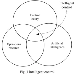
definitions of what is an intelligent control. In this paper a view of intelligent control as multidisciplinary domain in which control theory, artificial intelligence, and operations research intersected (Fig. 1) [23], is adopted. RL may be viewed as the domain where artificial intelligence and operations research intersected while CLF is a constructive control concept built upon rigorous theoretical considerations.
Control theory Operations research Artificial intelligence Intelligent control
Fig. 1 Intelligent control
In the paper, the emphasis is on how to combine these two concepts so as to achieve an intelligent control with respect to illustration in Fig. 1. In addition, it is argued that an intelligent control can become truly effective only if a domain-specific knowledge, or the knowledge about particular system (in this paper power system) and particular problem (oscillations damping) are fully exploited and incorporated in design of the control.
III. CONTROL LYAPUNOV FUNCTIONS:THEORETICAL BASICS The concept of CLF was introduced by Artstein [2] and Sontag [3]-[4] and had tremendous impact on stabilization theory [1]-[4]. Its main significance is the fact it converted stability descriptions into tools for solving stabilization tasks. To make this text self-contained, some results about the CLF from control theory [1]-[4] are briefly presented.
A. Continuous time systems
The discussion in this section largely follows that in [1], [2], [14]-[17]. Consider a nonlinear, affine in control, system,
n R x u x g x f u x f x ( , ) ( ) ( ) , . (1) One way to stabilize this system is to select a Lyapunov function
(x) and then to find a feedback control law u(x) that renders
(x,u(x)) negative definite [1], [2], [15]. If there exists a feedback control u u(x) defined in a neighborhoodq of the origin such that the closed-loop system x f(x,u(x)) has a locally asymptotically stable equilibrium point at the origin f(0,u(0)) then the system (1) is stabilizable at the origin and the function u u(x) is called a stabilizing feedback law. The function
(x), for the nonlinear system (1),is called CLF if [1], for all x 0,
0 x V L 0 x Lg
( ) f ( ) (2) where ( ): ( ) g(x) x x Lg and ( ): ( ) f(x) x x Lf .The existence of a CLF is necessary and sufficient condition for the stabilizability of a system with a control input. When
(x) is a CLF, there are many control laws that render
(x) negative definite [1]. This fact is considered in the paper as an opportunity rather than difficulty and more then one stabilizing control law is used for performance improvement purpose. The construction of a CLF is a hard problem, which has been solved for some special classes of systems [1]. Although a difficult task and still the subject of ongoing research [24], [25], the issue of finding Lyapunov functions candidates and construction of a CLF for a power system are not addressed in the paper. Instead, the results from [14]-[17] are largely followed.B. Discrete time systems
The definition of CLF for discrete time systems differs in details from the definitions for continuous-time systems. Below, slightly modified, definitions and a theorem adopted from [26] are given. Let a target set be T and let
R
:
such that
(x ) 0 for all x1T.Definition 1. The state of the system descends on
in 1 ifthere exists
0 such that for all xt1 holds that
(xt) (xt1) , where xtand xt1 are the system states at discrete time steps t and t+1, respectively.In other words, the state of the system descends on
if, from any xt1, the next state of the system is guaranteed to be lower on
by at least
or to be in the target set T. The function
is a Lyapunov function with target set T for a discrete time system if the state of the system descends on
.Theorem 1. If the state of the system descends on a Lyapunov
function
for all x1, then from any initial state1 0
x , the state of the system enters the target set T in at most
(x0)/
time steps.The proof of this theorem can be found in [26].
Definition 2.
is a CLF with target set T for a discrete timesystem if, for fixed
0 and all x T, there exists a control action that causes the state of the system to descent on
at least by amount
.C. Remarks
The definition 1 and 2 and theorem 1 provide strong guarantees on practical stability of the system. However, in practice it is often not possible to ensure that each state of the system be descending on
by any small amount. The conditions of definitions 1 and 2 and theorem 1 can be relaxed by allowing for some time steps the state of the system to benon-ascending on
(the concept of so-called weak CLF [19]) and the condition
(xt)
(xt1)
becomes0 x
xt) ( t1)
(
. For discussion on stability guarantees in this case interested readers are referred to [26].IV. REINFORCEMENT LEARNING
A control problem is considered here and natural choice of theoretical framework to present RL is to consider it as a way to learning (approximate) solutions of optimal control problems.
A. Theoretical framework
RL is presented here in the context of a deterministic time-invariant system, sampled at constant rate. If xtand utdenote the system state and control at time t, the state at time t+1 is given by, ) , ( t t 1 t f x u x , (3) where assumed that ut ,U t0 and that Uis finite.
To formulate the problem mathematically the framework of discounted infinite time horizon optimal control is used here. Let r(x,u)Bbe a reward function,
( 10, )a discount factor, and denote by u{t}(u0,u1,u2,...) a sequence of control actions applied to the system. The objective is to define, for every possible initial state x0, an optimal control sequence u{*t}(x0) maximizing the discounted return,
0 t t t t t 0 u r x u x R( , {}) ( , ). (4) One can show that these optimal control sequences can be expressed in the form of a single time-invariant closed-loop control policy u*(), i.e. ut*(x0)u*(xt),x0t0. In order to determine this policy one can define so-called the Q function [26], [27] by, )) , ( ( ) , ( ) , (x u r xu V f x u Q
, (5)where V(f(x,u))is the value function [27], [28], and deduce the optimal control policy,
) , ( max arg ) ( * x Q xu u U u , (6) by solving Bellman equation [28]. Equation (6) provides a straightforward way to determine the optimal control law from the knowledge of Q. RL algorithms estimate the Q function by interacting with the system.
B. State-space discretization and learning Q function
When the state-space is infinite (as in most power system problems) the Q function has to be approximated [27], [28]. In the considered applications, a state space discretization technique is used to this end. It consists in dividing the state space into a finite number of regions and considering that on each region the Q function depends only on u. Then, in the
RL algorithms, the notion of state used is not the real state of the system x but rather the region of the state space to which x belongs. Let the letter s to denote a discretized state, s(x) the
region to which the (true) state x belongs, and S the finite set of discretized states. Notice that the sole knowledge of the region s(xt) at some time instant t together with the control value u is not sufficient (in general) to predict with certainty the region s(xt1)to which the system will move at time t+1. This uncertainty is modeled by assuming that the sequence of discretized states followed by the system under a certain control sequence is a time-invariant Markov chain characterized by transition probabilities p(s's,u). Given these transition probabilities and a discretized reward signal, i.e. a function r( us, ), the initial control problem can be reformulated as a Markov Decision Process (MDP).
The corresponding Q function is characterized by the following Bellman equation,
S s u U u s Q u s s p u s r u s Q ' ) , ' ( max ) , ' ( ) , ( ) , ( , (7)the solution of which can be estimated by a classical dynamic programming algorithm like the value iteration or the policy iteration [27], [28]. The corresponding optimal control policy is extended to the original control problem, which is thus defined by the following rule,
) ), ( ( max arg )) ( ( ) ( * * x u s x Q s x u û U u . (8)
RL methods either estimate the transition probabilities and the associated rewards (model-based learning methods) and then compute the Q function, or learn directly the Q function without learning any model (non-model-based learning methods). For the purpose of this paper a model-based algorithm, known as prioritized sweeping [29], with -greedy
policy, is used. This policy consists in choosing with a probability a control action at random and with probability -1 the “optimal” control action associated with the current state
by the current estimate of Q function. The value of defines
the so-called “exploration-exploitation” tradeoff used by the algorithm [27], [30].
V. PROPOSED CONTROLS: THE PRINCIPLE
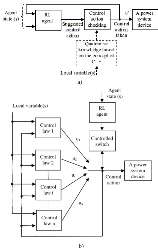
The conceptual diagrams of the proposed control schemes are illustrated in Fig. 2. In the first control scheme (Fig. 2a) a RL algorithm works in usual way [8]-[11] and at each time step suggests a control action in pursuit for the control sequence that minimizes pre-specified cost function (maximizes the discounted reward (4)). Each suggested control action is then checked for “safety” using qualitative knowledge about stabilizing control laws derived from the concept of CLF. If suggested control action satisfies certain criterion the action is taken, otherwise the control action is set to zero. The control action taken (indicated as urin Fig. 2a), at each time step, is passed back to the RL agent and together with other variables constitutes the RL agent state.
In the second control scheme (Fig. 2b) the system, as a whole, reveals itself as a switched system in which a switched controller is used to control the system. Two major tasks should be accomplished as a switched controller is designed [30]: (i) design of basic controllers (or control laws), and (ii) definition of switching law of the basic controllers. To solve the first task the concept of CLF is used and for the second one a RL algorithm is employed to determine a switching sequence of the basic control laws that minimizes a pre-specified cost function. Each individual control law u1,u2,...,un, is derived as a stabilizing continuous control law that renders a common (global) Lyapunov function candidate decreasing.
a) Local variable(s) Agent state (s) Control action Control law 1 RL agent A power system device Control law 2 Control law i Control law n u1 u2 ui un Controlled switch b)
Fig. 2 Conceptual diagram of the proposed controls
The aim of having active control signal as an input to each of the control laws is to allow that all the control laws always track each other such that “bumpless” switch from one control law to another is assured [31]. Smoothing the control in this manner eliminates chattering that may excite high frequency dynamics.
VI. STABILIZING CONTROL LAWS FOR A TCSC[13]-[16] The results from [14]-[17], where the control strategies for damping of power oscillations based on the CLF concept were considered, are largely followed. The energy function of uncontrolled system, for reduced network model, was used as a Lyapunov function candidate in all [14]-[17]. This approach is known, in control theory, as Jurdjevic-Quinn control [32] or damping control for stable systems where the uncontrolled
system is stable and the task of the control is to provide additional damping.
Following the results from [14]-[17] the stabilizing control laws of the TCSC’s reactance reference can be formalized as,
) ( lm lm
ref F V V
X , (9) where F(VlmVlm)0 for VlmVlm 0, F(VlmVlm)0 for
0 V
Vlmlm , and F(0)0. In (9) Vlm is the magnitude of the voltage drop across the line l-m where the TCSC is installed. Voltage Vlm is locally measurable. If the line has impedance Xlm then, TCSC lm lm lm X I V V , (10) where VTCSC is the magnitude of the voltage drop across the TCSC. Vlm can be inferred based upon tracking of Vlm. A wide range of possible choices for the control function
) (VlmVlm
F can be used [16]. Different possibilities for the control function were addressed in [16]. In [14]-[17] only linear, continuous control functions were considered.
An important observation is that the control laws are based on locally measurable quantities. This facilitates the definition of target set, introduced in section III.B, which will be considered as a small neighborhood of
F
where the CLF-based control is not active.VII. DESCRIPTION OF THE TEST POWER SYSTEM MODEL To illustrate capabilities of the proposed control schemes to control a TCSC the four-machine power system model [22] described in Fig. 3, is used.
5 1 6 7 8 3 4 2 9 10 G3 G4 G2 G1 L7 L10 TCSC
Fig. 3 A four-machine power system
Input signals Control strategy Xmin Xmax s 06 0 1 1 . ref X
Fig. 4 Block diagram of the TCSC
All the machines are modeled with a detailed generator model, slow direct current exciter, automatic voltage regulator, and speed regulator. The loads are modeled as constant current (active part) and constant impedance (reactive part). The TCSC is considered as a variable reactance placed in series with a transmission line. The block diagram of TCSC considered is illustrated in Fig. 4. The control variable is Xref
value of –61.57 for TCSC reactance corresponds approximately to 30% compensation of the line on which the device is installed.
The results of two case studies are presented. CLF-based control laws are damping controls but which do not directly take into account system performance. In presented case studies introducing a cost function, that a RL method tries to minimize over time and balance between system stability and performance, further extends these controls. To implement the control schemes the state and reward for the RL algorithm as well as the rule for checking control actions and a set of basic control laws have to be defined.
In both case studies the same target set is used for CLF- based control and is defined as,
} . | ) {(V V V V 001 T lm lm lmlm (11) VIII. CASE STUDY I
This case study focuses on how to control a TCSC using the control scheme illustrated in Fig. 2a.
A. State and reward definition
The control scheme, as a whole, is supposed to rely on strictly locally measurable information and a minimal set of a single local measurements (in addition to those required by CLF control) is chosen, namely of the active power flow through the line in which the device is installed. This quantity is obtained at each time step of 50ms. It is used to define the rewards and pseudo-states used by the RL algorithm. To cope with partial observability of the system the approach considered in [11] is adopted and a pseudo-state from the history of the measurements and actions taken is defined. The pseudo-state at time t is defined by the following expression,
r
t 1 t 1 et et t P P u u s , , , . (12) The aim of the control is to maximize damping of the electrical power oscillations in the line with as less as possible control efforts. In this respect, the reward is defined by, 250 10 P P if 1000 u u if 1000 u u if u c 10 P P r 6 e et r t t r t t t 6 e et t / / . (13)
where Pe represents an estimate of the steady-state value of the electric power transmitted through the line, the condition
250 10 P
Pet e / 6 is used to detect instability, and parameter c penalizes the value of the control.
Note that the steady state value of the electrical power is dependent on several aspects (operating point, steady state value of Xref indicated in Fig. 4) and so cannot be fixed
beforehand. Thus, rather than to use a fixed value of Pe, its value is estimated on-line using the following equation,
1199 0 i i 1 et e P 1200 1 P , (14)which is a moving average over the last 1200*50ms=60s and provides the algorithm with some adaptive behavior.
It is important to note that the instability detection is included in the reward (13). This is due to the fact that to different discrete values of Xref correspond different stability
domains and stability of any sequence of applied control actions cannot be guaranteed in this setting (particularly at the beginning of the learning). Consequently, this control scheme cannot be applied in on-line mode directly. Biasing of the control in simulation environment or initialization of the Q function by supplying a good heuristic control policy prior its on-line application is necessary.
B. The rule for suggested control actions checking
This rule is derived directly from the results discussed in Section VI. The results reveal that the TCSC’s reactance has to be controlled in such a way that it matches the sign of the product VlmVlm and the rule is formalized as follows,
otherwise 0 T V V and 0 V V and 0 u or T V V and 0 V V and 0 u if u u lm lm lm lm t lm lm lm lm t t r t ) ( ) ( (15) Each “accepted” control action is passed through a low-pass filter, before being applied, with the purpose of chattering problem elimination.
C. The value of parameters
The control set is discretized in four values equal to
U={-61.57,-41.05,-20.54,0.} while electrical power transmitted in the line is discretized in 100 values within interval [-250,250]MW. The parameters are set to =0.98,
=0.05 (preliminary simulations and results from [11] revealed
these values as appropriate), and c=0.5.
D. Simulation results
The system response to the 100 ms duration, three-phase self-cleared short circuit near bus 7 on the lower line (Fig. 3) between the buses 7 and 10, is shown in Fig. 5 (the speed of G2 relative to G3). From Fig. 5 it is clear that the system becomes unstable through growing inter-area oscillations of about 0.72 Hz.
The learning period is partitioned into different scenarios. Each scenario starts with the power system being at rest and is such that at 1s the self-cleared short-circuit near bus 7 occurs. The simulation then proceeds in the post-fault configuration until t is greater than 60s. The progressive learning is illustrated in Fig. 6a.
The controlled system responses after the first learning scenario (dotted), after 100 (dot-dashed), 300 (solid), and 350 (solid) learning scenarios together with the response under a
standard CLF-based linear control law (dashed, )
( km km
ref k V V
X , k5.0), are shown.
Fig. 5 The response of the uncontrolled system
a)
b) c)
Fig. 6 The response of the controlled system (a), control actions u (b), and tr electrical power in the line (c)
When the fault is met for the first time, the controller succeeds to stabilize the system (although this is not guaranteed in the beginning of the learning process) but oscillations are rather poorly damped. After 100 learning scenarios the controller outperforms standard CLF-based control. The results are more pronounced after 300 and 350 scenarios. The system responses after 300 and 350 scenarios are almost identical indicating that the RL algorithm converged to a good approximation of an optimal control policy. The variation of the control variable and electrical power in the line, after 350 learning scenarios, is illustrated in Fig. 6b and Fig. 6c.
To illustrate how the control scheme accommodates changing system operating conditions, the system is subjected to the same fault type with the fault duration increased to 120
ms and slightly modified pre-fault conditions (active power
productions of the generators G1 and G2 are increased by the amount of 10 MW). The system response is shown in Fig. 7 (dashed). The controller successfully stabilized the system. Moreover, the control scheme benefits from additional scenarios of the same type and the system response after 20 additional scenarios is shown in Fig. 7 (solid).
Fig. 7 The controlled system responses to an “unseen” fault IX. CASE STUDY II
This section illustrates the capabilities of the control scheme depicted in Fig. 2b in controlling the same device.
A. Basic control laws
For the simulation purposes four linear, continuous control laws are used (see section VI). The slope of the control laws is chosen based on preliminary simulations and observations given in [14], [15], and for the control laws,
) ( ) ( lm lm lm lm ref F V V k V V X u , (16)
four values of parameter k=(5.0,6.0,7.0,8.0) are considered. In this setting an approximation of the optimal sequence of parameter k is to be learned.
Stability guarantees hold for any sequence of k within the stability domain determined by limiting values of the control and, in principle, this control scheme can be applied in on-line mode directly.
B. State and reward definition
To retain locality of the overall control scheme the measurements of the active power flow in the line where the TCSC is installed are again used as inputs to the RL algorithm. The pseudo-state at time t is defined as,
et et 1 et 2 t 1 t 2
t P P P k k
s , , , , . (17) Since the aim of the control is the same as in the case study I, the reward is defined as,
t 6 e et t P P 10 c u r / (18) The same parameters of the learning algorithm and discretization of the power flow, as in case study I, are used.
C. Simulation results
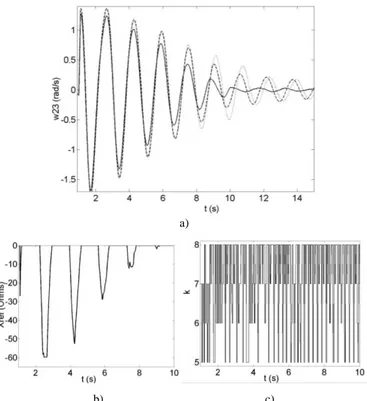
The controlled system responses when subjected to the same fault as in the previous case study, with the TSCS
controlled by CLF-based control for k=5.0 (dotted) and k=8.0 (dashed) are given in Fig. 8a. In the same figure the response of the system being controlled by the proposed control scheme after 350 learning scenarios, is presented (solid). The learning scenarios are the same as defined in the case study I. Note that the proposed control scheme considerably improves the oscillations damping and the settling time is quite smaller than in the case of standard CLF- based controls.
a)
b) c)
Fig. 8 The controlled system response: CLF with k=5.0 (dotted), k=8.0 (dashed), and after 350 learning scenarios (solid) (a), control efforts (b) and
sequence of k (c).
The “bumpless” non-excessive control law is achieved (Fig. 8b). Assuring “bumpless” switch from one control law to another is, in general nonlinear systems, a rather formidable task. However, in this case study it is extremely simplified due to the fact that all stabilizing control laws have the same analytical form and “bumpless” switch is simply realized through the use of a low-pass filter placed behind the switch. The sequence of the values of k is illustrated in Fig. 8c.
When the same RL algorithm is used alone (without limiting controls to be stabilizing) to control the system, for the same learning scenarios, the control algorithm is not able to stabilize the system rather often. In the simulations carried out (120 scenarios) the control set is discretized in four values
U={-61.57,-41.05,-20.54,0.} while other parameters are kept the
same as in other simulations included in this paper. The cumulative number of times the system loses stability as a function of the number of learning scenarios is represented in Fig. 9. No one unstable case was met by applying the proposed constructive intelligent control scheme.
Fig. 9 Number of unstable scenarios when RL control is used alone X. DISCUSSION
Stability guarantees in the proposed control schemes are ensured by design, i.e. by imposing Lyapunov-based constraints on the available control choices to the RL algorithm. These guarantees hold regardless of particular RL algorithm used. The CLF-based basic control laws for the TCSC do not include any parameter, which is dependent on the network conditions, and the control response is robust with respect to system loading, network topology, and fault type and location [14]-[17]. However, the RL algorithm is used to learn an approximation of the optimal sequence of the basic control laws and to each power system configuration corresponds an optimal sequence. Thus, each time the controller faces a structural change in the system it must learn a new approximation, and may “forget” the learned policy for other system configurations. This is the reason prioritized sweeping algorithm is used because this algorithm, according to our experience [8], [11], [12], makes more efficient use of data gathered, finds better policies, and handle changes in the environment more efficiently. Although, in principle, the choice of RL algorithm is not an issue the proper choice of the algorithm plays an important role in ensuring overall control scheme flexibility and adaptivity.
Prioritized sweeping RL algorithm solves the problem just partly and this is certainly the issue to be tackled in the future research. Fortunately, the research in the field of RL is very intensive and more and more powerful algorithms are at our disposal and should be considered in the future research to find those able to cope with the problem more efficiently.
For a formal proof of the prioritized sweeping RL algorithm convergence, interested readers are referred to [33] where a generalized RL method was considered and a new stochastic approximation theorem is introduced. This theorem implies the convergence of the algorithm.
Observe that any meaningful cost function, by appropriate reward definition, can be used in the proposed control.
Derivation of CLF-based control laws [14]-[17] were based on domain-specific knowledge rather than Sontag’s universal formulae [4]. Moreover, by imposing Lyapunov-based constraints on available controls the domain-specific
knowledge is incorporated into RL method.
XI. SOME FUTURE RESEARCH DIRECTIONS
Highlighting the benefits of applying a constructive intelligent control in solving power system control problems is primary aim of this paper. Some important issues are not considered and will be tackled within future research efforts.
There is a space for improvement in both CLF and RL application in power system control. Research opportunities in RL applications are discussed briefly in previous section. As of the CLF concept research possibilities may include: extension of the concept from [14]-[17] by considering recently introduced extended Lyapunov function [23] for power system, using the concept of robust CLF [19], and casting the problem as an inverse optimal control [19]. Furthermore, all control laws derived in [14]-[17], and used in this paper, are derived without explicit account for bounds on control signals. Theoretical results given in [34] offer a sound solution to this problem and are worth further consideration. In addition, Jurdjevic-Quinn approach [32] used in [14]-[17] has a limitation [35] that stems from the fact that Lyapunov function candidate is chosen for the uncontrolled system in complete disregard of the flexibility that may be offered by the control term g(x)u in (1). More systematic approaches are now available to resolve this problem [35].
This text mentioned RL applications in power system control as of 2006. For a recent account of these applications, interested readers are referred to [36]. In a way, this text also complements the work of [36], in particular related to safety issues in RL applications in power system control.
XII. CONCLUSIONS
Constructive intelligent control based on an appropriate combination of the methodologies from control theory and artificial intelligence, together with the domain-specific knowledge, is a promising way to implement advanced control techniques to solve power system control problems. In this text that complements materials presented in [1,2], it is demonstrated by the combination of the RL algorithm and the concept of the CLF. The two control schemes were presented and their capabilities illustrated on the control problem involving a TCSC for damping oscillations in the system.
The main advantages of the proposed control schemes to either standard RL or CLF-based methods alone are: by imposing Lyapunov-based constraints on the control set it has been made possible to apply RL in on-line mode and by using a RL method the system performance over a set of stabilizing control laws has been improved. Thus, the objective of optimizing a mix of stability and performance is achieved.
Although only the control of a TCSC device is considered in the paper, the proposed approach is equally applicable to other types of flexible AC (alternating current) transmission systems devices such as static var compensators (SVC) and static compensators (STATCOM). Moreover, it has been shown in [14-17] that different devices with CLF control do
not adversely affect each other. This offers the proposed approach as an attractive one to design the multi-agent intelligent control systems.
In principle, any control with stability guarantees can be combined with the RL methods and any heuristic search technique can be combined with the CLF-based control in a similar way.
XIII. REFERENCES
[1] M. Glavic, D. Ernst, L. Wehenkel, “Combining a Stability and a Performance Oriented Control in Power Systems”, IEEE Transactions on Power Systems, vol. 20, no. 1, pp. 525-527, 2005.
[2] M. Glavic, D. Ernst, L. Wehenkel, “Damping Control by Fusion of Reinforcement Learning and Control Lyapunov Functions”, In Proc. North American Power Symposium, NAPS, Carbondale, IL, USA, 2006. [3] P. Kokotovic, M. Arcak, “Constructive Control: A Historical
Perspective”, Automatica, Vol. 37, pp. 637-662, 2001.
[4] Z. Artstein, “Stabilization with Relaxed Controls”, Nonlinear Analysis, Vol. 7, No. 11, pp. 1163-1173, 1983.
[5] E. D. Sontag, “A Lyapunov-like Characterization of Asymptotic Controllability”, SIAM Journal of Control and Optimization, Vol. 21, pp. 462-471, 1983.
[6] E. D. Sontag, “A ‘Universal’ Construction of Artstein’s Theorem on Nonlinear Stabilization”, System and Control Letters, Vol. 13, No. 2, pp. 117-123, 1989.
[7] A. G. Phadke, “Synchronized Phasor Measurements in Power”, IEEE Computer Applications in Power, Vol. 6, No. 2, pp 10-15, 1993 [8] D. Ernst, M. Glavic, P. Guerts, L. Wehenkel, “Approximate Value
Iteration in the Reinforcement Learning Context. Application to Electrical Power System Control”, International Journal of Emerging Electric Power Systems, vol. 3, no. 1, article 1066, 2005.
[9] J. Jung, C. C. Liu, S. L. Tanimoto, V. Vittal, “Adaptation in Load Shedding Under Vulnerable Operating Conditions”, IEEE Transactions on Power Systems, Vol. 17, No. 4, pp. 1199-1205, 2002.
[10] C. C. Liu, W. Jung, G. T. Heydt, V. Vittal, A. G. Phadge, “The Strategic Power Infrastructure Defense (SPID) System”, IEEE Control System Magazine, Vol. 20, pp 40-52, 2000.
[11] D. Ernst, M. Glavic, L. Wehenkel, “Power System Stability Control: Reinforcement Learning Framework”, IEEE Transactions On Power Systems, Vol. 19, No. 1, 2004.
[12] M. Glavic, “Design of a Resistive Brake Controller for Power System Transient Stability Enhancement using Reinforcement Learning”, IEEE Transactions on Control Systems Technology, vol. 13, no. 5, pp. 743-752, 2005.
[13] M. Glavic, D. Ernst, L. Wehenkel, “A reinforcement learning based discrete supplementary control for power system transient stability enhancement”, In Proc. Intell. Syst. Applic. in Power, Paper ISAP2004/017, Lemnos, Greece, 2003.
[14] M. Ghandhari, G. Andersson, M. Pavella, D. Ernst, “A control strategy for controllable series capacitor in electric power systems”, Automatica, Vol. 37, pp. 1575-1583, 2001.
[15] M. Ghandhari, G. Andersson, I. A. Hiskens, “Control Lyapunov Functions for Controllable Series Devices”, IEEE Trans. on Power Systems, Vol. 16, No. 4, pp. 689-694, 2001.
[16] J. F. Gronquist, W. A. Sethares, F. L. Alvarado, R. H. Lasseter, “Power oscillations damping control strategies for FACTS devices using locally measurable quantities”, IEEE Transactions on Power Systems, Vol. 10, No. 3, pp. 1598-1605, 1995.
[17] M. Noroozian, M. Ghandhari, G. Andersson, J. Gronquist, I. Hiskens, “A Robust Control Strategy for Shunt and Series Reactive Compensators to Damp Electromechanical Oscillations”, IEEE Transactions on Power Delivery, Vol. 16, No. 4, pp. 812-817, 2001. [18] P. J. Werbos, “Stable Adaptive Control Using New Critic Designs”,
[Online]. Available: http://arxiv.org/html/adap-org/9810001, 1998. [19] R. A. Freeman, P. V. Kokotovic, “Inverse Optimality in Robust
Stabilization”, SIAM Journal of Control and Optimization, Vol. 34, pp. 307-312, 1996.
[20] V. L. Rawls, R. A. Freeman, “Adaptive Minimum Cost-Lyapunov-Descent Control of Nonlinear Systems”, In Proc. of American Control Conference, Chicago, USA, pp. 1649-1653, 2000.
[21] J. J. Murray, C. J. Cox, G. G. Lendaris, “Adaptive Dynamic Programming”, IEEE Trans. on Systems, Man, and Cybernetics – Part C: Applications and Reviews, Vol. 32, No. 2, pp. 140-153, 2002. [22] P. Kundur, Power System Stability and Control, McGraw Hill, 1994 [23] G. N. Saridis, “Foundations of the Theory of Intelligent Controls”, In
Proc. of the IEEE Workshop on Intelligent Control, Troy, New York, USA, pp. 23-28, 1985.
[24] N. G. Bretas, L. F. C. Alberto, “Lyapunov Function for Power Systems with Transfer Conductances: Extension of the Invariance Principle”, IEEE Trans. on Power Systems, Vol. 18, No. 2, pp. 769-777, 2003. [25] R. J. Davy, I. A. Hiskens, “Lyapunov Functions for Multimachine
Power Systems with Dynamic Loads”, IEEE Trans. on Circuits and Systems – I: Fundamental Theory and Applications, Vol. 44, No. 9, 1997.
[26] T. J. Perkins, A. G. Barto, “Lyapunov Design for Safe Reinforcement Learning”, Journal of Machine Learning Research, Vol. 3, pp. 803-832, 2002.
[27] R. S. Sutton, A. G. Barto, Reinforcement Learning: An Introduction, MIT Press, 1998.
[28] D. P. Bertsekas, J. N. Tsitsiklis, Neuro-Dynamic Programming, Athena Scientific, Belmont, MA, 1996
[29] R. Bellman, Dynamic Programming, Princeton University Press, 1957 [30] A. W. Moore, C. G. Atkeson, “Prioritized sweeping: Reinforcement
learning with less data and less real time”, Machine Learning, vol. 13, pp. 103-130, 1993.
[31] Z. G. Li, C. Y. Wen, Y. C. Soh, “Switched Controllers and Their Applications in Bilinear Systems”, Automatica, Vol. 37, pp. 477-481, 2001.
[32] V. Jurdjevic, J. P. Quinn, “Controllability and Stability”, Journal of Differential Equations, Vol. 28, pp. 381-389, 1978.
[33] M. L. Littman, C. Szepesvari, “A Generalized Reinforcement Learning Model: Convergence and Applications”, In Proc. of International Conference on Machine Learning ICML-96, pp. 310-318, 1996. [34] Y. Lin, E. Sontag, “Control Lyapunov Univesal Formulae for restricted
inputs”, International Journal of Control Theory and Advanced Technology, Vol. 12, pp. 1981-2004, 1995.
[35] R. Sepulchre, M. Jankovic, P. Kokotovic, Constructive Nonlinear Control, Springer-Verlag, 1997.
[36] M. Glavic. R. Fonteneau, D. Ernst, “Reinforcement Learning for Electric Power System Decision and Control: Past Considerations and Perspectives”, IFAC-PapersOnLine, Vol. 50, No. 1, pp. 6918-6927, July 2017.