HAL Id: tel-00798576
https://tel.archives-ouvertes.fr/tel-00798576
Submitted on 8 Mar 2013HAL is a multi-disciplinary open access archive for the deposit and dissemination of sci-entific research documents, whether they are
pub-L’archive ouverte pluridisciplinaire HAL, est destinée au dépôt et à la diffusion de documents scientifiques de niveau recherche, publiés ou non,
Statistical Post-Processing Methods And Their
Implementation On The Ensemble Prediction Systems
For Forecasting Temperature In The Use Of The French
Electric Consumption
Adriana Geanina Gogonel
To cite this version:
Adriana Geanina Gogonel. Statistical Post-Processing Methods And Their Implementation On The Ensemble Prediction Systems For Forecasting Temperature In The Use Of The French Electric Con-sumption. General Mathematics [math.GM]. Université René Descartes - Paris V, 2012. English. �NNT : 2012PA05S014�. �tel-00798576�
Université Paris Descartes
Laboratoire MAP 5École Doctorale de Sciences Mathématiques de Paris Centre THÈSE
pour obtenir le grade de
Docteur en Mathématiques Appliquées
de l’Université Paris Descartes Spécialité : STATISTIQUE
Présentée par Adriana CUCU GOGONEL
Statistical Post-Processing Methods And Their Implementation On The Ensemble Prediction Systems For Forecasting Temperature In The Use Of The French Electric
Consumption. Thèse dirigée par
Avner BAR-HEN
soutenue publiquement le 27 novembre 2012
Jury
Rapporteurs Jerome Saracco, Institut Polytechnique de Bordeaux Jocelyn Gaudet, Hydro-Québec
Examinatrice Virginie Dordonnat, EDF R&D
Examinateur Eric Parent, AgroParisTech/INRA
Directeurs de thèse Avner Bar-Hen, Université Paris Descartes
Remerciements
Je voudrais en premier lieu remercier les personnes qui ont rendu possible l’existence de cette thèse, je pense à mon directeur de thèse, Avner Bar-Hen et à mon encadrant EDF, Jérôme Collet. Je remercie Avner d’avoir bien voulu assumer la direction de cette thèse. Son soutien, sa bonne humeur, sa disponibilité et son exigence ont été des éléments indis-pensables à la réussite de ce travail. Je remercie Jérôme qui m’a fait découvrir la recherche et m’a donné le gout du SAS. Il a toujours su se rendre disponible et me faire bénéficier de son expérience tout en me laissant une grande liberté d’action.
Je tiens à exprimer ma gratitude aux personnes qui m’ont fait l’honneur de participer au jury de cette thèse. Je suis reconnaissante envers Jérôme Saracco et Jocelyn Gaudet pour l’intérêt qu’ils ont porté à cette thèse en acceptant d’en être les rapporteurs, leurs rapports m’ont permis d’améliorer ce manuscrit. Je suis particulièrement reconnaissante à Virginie Dordonnat, pour ses conseils précieux dans tous les domaines : technique, métier, valorisation du travail, écriture du rapport ainsi que pour son soutien continu qui a été d’autant plus précieux dans mes moments de doutes. Je tiens à remercier également Eric Parent de m’avoir fait part de ses idées sur mes travaux, ce qui m’a ouvert des perspectives pour la suite de la thèse.
Je remercie mes collègues Julien Najac, Laurent Dubus, Thi-Thu Huong-Hoang, Christophe Chaussin et Marc Voirin d’avoir participé aux réunions de suivi de ma thèse. Ces réunions ont toujours été d’une aide importante dans l’évolution des travaux de thèse. Je remercie Thi-Thu pour son aide sur la partie des valeurs extrêmes de la thèse ainsi que pour sa gentillesse et sa disponibilité.
Je tiens ensuite à remercier Sandrine Charousset et François Regis-Monclar qui m’ont permis de démarrer cette thèse à EDF R&D. Je remercie également Bertrand Vignal et plus particulièrement Marc Voirin qui ont supervisé le bon déroulement de ma thèse ainsi que mon intégration dans l’équipe R32 du département OSIRIS. Ils m’ont encouragée tout en mettant à ma disposition des conditions de travail idéales. Je remercie également Laetitia Hubert et Christelle Roger qui m’ont soutenue dans mes démarches administratives.
J’ai une pensée pour tous les membres du département OSIRIS que j’ai eu le plaisir de côtoyer durant ces quatre années de thèse ainsi qu’au cours de mon stage de Master 2. Une pensée plus particulière va à Xavier Brossat qui m’a fait découvrir la beauté des con-férences et le charme de Prague et à qui j’ai fait découvrir le "talent de buveuse" des filles de l’est !
Je remercie mes collègues de bureau pendant les quatre années, par ordre chronologique : Laurence pour le plein de conseils sur le fonctionnement de la R&D et sur la vie d’une maman-chercheur, Codé pour sa bonne humeur permanente et pour ses chansonnettes, Nicolas pour les discussions sport et pas que et Kuon pour sa sagesse et son optimisme, à mon égard.
Je tiens à remercier mes collègues de la "tant aimée" équipe R32, pour leur bonne humeur, pour leur soutien. Ils m’ont appris tellement de choses sur des domaines différents, ma culture générale s’est améliorée à leur coté et ils m’ont sûrement donné envie d’être un bon ingénieur. Je vais avoir du mal à retrouver ailleurs un autre Dominique, toujours à l’écoute, discret mais toujours présent avec un bon conseil. Un remerciement particulier à Sabine pour son soutien, toujours prête à m’aider et à m’écouter, j’aurais aimé savoir en profiter plus. Je voudrais également remercier Bogdan, mon cher collègue roumain, un mélange parfait de professionnalisme et de joie. Je remercie Jérôme et Jérémy de m’inciter puis m’écouter parler des exploits sportifs de mon époux. Je tiens à remercier Sébastien, ses conseils sur le timming dans l’écriture de rapport m’ont été d’un réel aide, mais c’est quand même son humour noir qui l’emporte dans mes souvenirs. Je voudrais également remercier Aline, nos échanges lors de mon arrivée à EDF resterons toujours dans ma mémoire. J’ai une pensée également pour Muriel qui m’a apporté un vrai soutien à mon retour de congé de maternité. Je remercie Florent pour nos discussions détendues mais tout aussi intéressantes et puis pour les discussions "bébé". Plus particulièrement je voudrais remercier Pascale, un exemple d’élégance et de professionnalisme, et un mélange très réussi de sérieux et de folie. Je remercie également Mathilde, Thi-Thu et Virginie pour leurs encouragements et leurs conseils d’autant plus précieux qu’ils viennent de leurs ré-centes expériences de doctorantes. Je voudrais remercier Avner, Jérôme, Virginie, Sabine, Xavier, Olivier, Thi-Thu et Lili pour leur aide dans l’amélioration de mes transaparents de soutenance et du discours qui les accompagne, j’espère qu’ils seront contents du résultat! Cette section ne serait pas complète si je ne remerciais pas mes amies de l’université, Lian, Nathalie et Souad à côté desquelles j’ai découvert les statistiques. Elles sont sûrement plus capables que moi de faire une thèse. Bien que ce soit moi qui l’ai faite finalement c’est comme si cette thèse était un peu la leur. Je profite pour remercier nos professeurs de Paris 5, pour les connaissances qu’ils ont su si bien nous transmettre et pour leur accueil chaleureux lors de mon arrivée en thèse.
Je tiens à exprimer mes remerciements aux amis du kyokushin qui m’ont aidée, par la folie de leur jeunesse, à m’échapper de temps en temps aux doutes de la thèse. Je remercie Djéma pour son humour contagieux, Guillaume pour ses compliments culinaires et Yacine pour son éternelle gentillesse !
Je voudrais remercier mes amis roumains, même s’ils sont loin, ils m’ont soutenue et encouragée tout au long de cette période de thèse. Je remercie Marian C pour ses con-seils judicieux, toujours bien intentionnés, Aura S pour sa façon unique de me rassurer et Bianca C de m’avoir partagé son expérience de gestion d’une thèse en tant que maman. Je remercie également Mihaela B pour ses conseils avisés et son attitude sans retenue envers une ancienne étudiante. Je tiens à remercier mon professeur de mathématique au collège, Ion Lixandru, de m’avoir fait aimer les maths et de m’avoir donné confiance en moi. Je remercie Veronica -qui m’amène ici un peu de Roumanie- pour son énergie débordante, que j’aimerais tant lui piquer !
Mes derniers remerciements vont vers ma famille. Je remercie mes parents de la richesse de ce qu’ils ont su me transmettre, c’est sans doute la base de toutes les réussites de ma vie. Je remercie Lili, ma s œur et meilleure amie, de n’avoir jamais cessé de croire en moi et de m’avoir porté bon conseil dans toutes les décisions que j’ai dû prendre dans ma vie et dans mes études en particulier. Sans son aide ma vie aurait été sûrement moins simple et le chemin vers le bonheur beaucoup plus long. Je tiens à remercier Sam pour nos échanges enrichissants dans de si nombreux domaines. J’ai toujours pu m’appuyer sur son épaule et ses conseils m’ont souvent inspiré. Je remercie également Claude pour sa présence apaisante qui m’a toujours donné confiance. Une pensée émue va à mon neveu, Mathis et à ma nièce Julia, nés pendant mes années de thèse, qui j’espère liront un jour avec intérêt ce manuscrit !
Un remerciement particulier à Lucian, mon cher champion et le grand sage de la famille. Son soutien sans faille et sa patience pendant ces années de thèse m’ont été d’une aide précieuse. Il a su m’encourager, me donner envie d’avancer et me conseiller des breaks quand mon état le montrait. Je lui remercie aussi pour un cadeau très spécial en deuxième année de thèse, notre fils, Thomas, que je remercie de m’avoir fait découvrir la douce maternité en même temps que la recherche.
Résumé
L’objectif des travaux de la thèse est d’étudier les propriétés statistiques de correction des prévi-sions de température et de les appliquer au système des préviprévi-sions d’ensemble (SPE) de Météo France. Ce SPE est utilisé dans la gestion du système électrique, à EDF R&D, il contient 51 membres (prévisions par pas de temps) et fournit des prévisions à 14 jours. La thèse comporte trois parties. Dans la première partie on présente les SPE, dont le principe est de faire tourner plusieurs scénarios du même modèle avec des données d’entrée légèrement différentes pour simuler l’incertitude. On propose après des méthodes statistiques (la méthode du meilleur membre et la méthode bayésienne) que l’on implémente pour améliorer la précision ou la fiabilité du SPE dont nous disposons et nous mettons en place des critères de comparaison des résultats. Dans la deuxième partie nous présentons la théorie des valeurs extrêmes et les modèles de mélange et nous proposons des modèles de mélange contenant le modèle présenté dans la première partie et des fonctions de distributions des extrêmes. Dans la troisième partie nous introduisons la régression quantile pour mieux estimer les queues de distribution.
Mots clés: Prévisions de température, systèmes de prévisions d’ensemble, méthode du meilleur membre, critères de validation des SPE, théorie des valeurs extremes, modèles de mélange, re-gréssion quantile.
The thesis has for objective to study new statistical methods to correct temperature predictions that may be implemented on the ensemble prediction system (EPS) of Meteo France so to improve its use for the electric system management, at EDF France. The EPS of Meteo France we are working on contains 51 members (forecasts by time-step) and gives the temperature predictions for 14 days. The thesis contains three parts: in the first one we present the EPS and we implement two statistical methods improving the accuracy or the spread of the EPS and we introduce criteria for comparing results. In the second part we introduce the extreme value theory and the mixture models we use to combine the model we build in the first part with models for fitting the distributions tails. In the third part we introduce the quantile regression as another way of studying the tails of the distribution.
Keywords: Temperature forecasts, ensemble prediction systems, best member method, EPS validation criteria, extreme value theory, mixture models, quantile regression.
Contents
Version abrégée 11
Summary 15
Publications and Conferences 19
1 Introduction 21
1.1 Context and Data Description . . . 22
1.1.1 Context . . . 22
1.1.2 Data Description . . . 24
1.2 Ensemble prediction systems (EPS) . . . 28
1.2.1 History and building methods . . . 28
1.2.2 Forecasts and uncertainty in meteorology . . . 29
Sources of forecast errors . . . 30
1.3 The verification methods for EPS . . . 31
1.3.1 Standard Statistical Measure . . . 31
Bias . . . 31
Correlation coefficient . . . 31
Mean absolute error (MAE) . . . 32
The root mean square error (RMSE). . . 32
1.3.2 Reliability Criteria . . . 32
Talagrand diagram . . . 32
Probability integral transform (PIT) . . . 33
Reliability Diagram . . . 33
1.3.3 Resolution (sharpness) Criteria . . . 34
Brier Score . . . 34
Continuous Rank Probability Score (CRPS) . . . 34
Ignorance Score . . . 35
ROC Curve . . . 35
1.4 Post-processing methods . . . 36
1.4.1 The best member method . . . 36
The weighted members method . . . 37
1.4.2 Bayesian model averaging . . . 38
2 Implementation of two Statistic Methods of Ensemble Prediction Systems for Electric System Management (CSBIGS Article) 41 3 Mixture Models in Extreme Values Theory 61 3.1 Extreme Value Theory . . . 62
3.1.1 Peaks Over Thresholds . . . 64
Choice of the threshold . . . 65
Dependence above threshold . . . 66
3.2 Mixture models . . . 67
3.2.1 Parameter estimation . . . 68
Method of Moments . . . 68
Bayes Estimates . . . 68
Maximum Likelihood Estimation . . . 69
The Expectation Maximization algorithm . . . 69
3.3 Mixture models in the Extreme Value Theory . . . 71
3.4 The proposed extreme mixture model . . . 72
3.5 Implementation of the Extreme Value Theory on Temperature Forecasts Data . . 74
3.5.1 Context and Data . . . 74
3.5.2 Choices of extreme parameter values . . . 75
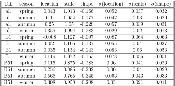
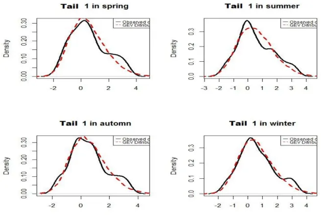
3.5.3 Mixture model and criteria of comparison of the final distributions . . . . 80
Mixture Models with the GEV parameters estimated by tail and by season 80 Mixture Models with the EVT parameters estimated by tail and for the right tail, by time-horizon. . . 81
Mixture Models with the GEV parameters estimated by tail, by month and by package of time-horizon. . . 95
Discussion extreme mixture models . . . 96
4 Improvement of Short-Term Extreme Temperature Density Forecasting using Best Member Method (NHESS Article) 99 Conclusion 105 Appendix 109 Case of the Extreme Values given by the 1st and 51st rank . . . 123
List of Figures 128
Version abrégée
Ces travaux sont réalisés dans le cadre d’une thèse CIFRE entre l’Université Paris Descartes (Laboratoire MAP5) et le département OSIRIS de la R&D d’EDF.
L’objectif des travaux de la thèse est d’étudier les propriétés statistiques de correction des prévi-sions de température et de les appliquer au système des préviprévi-sions d’ensemble (SPE) de Météo France pour améliorer son utilisation pour la gestion des systèmes électriques, à EDF R&D. Le SPE de Météo France que nous utilisons contient 51 membres (prévisions par pas de temps) et fournit des prévisions pour 14 horizons (un horizon est le pas de temps pour lequel une prévision est faite, et il correspond à 24 heures), pour une période de 4 ans: de mars 2007 à mars 2011. C’est une étude univariée, dans le sens où tous les horizons ne seront pas traités en même temps et que les méthodes portent sur un seul horizon à la fois. Néanmoins nous implémentons les méthodes choisies pour les horizons de 5 à 14 indépendemment. Nous n’intégrons pas à notre étude les horizons de 1 à 4, car les prévisions de témpérature détérministes sont très bonnes dans ce cas.
La thèse comporte trois parties: une première grande partie où on présente les SPE, les méth-odes statistiques proposées (et leur implémentation) pour améliorer la précision ou la fiabilité du SPE et les critères de comparaison des résultats. Dans la deuxième partie nous proposons des modèles de mélange du modèle présenté dans la première partie et des fonctions de distributions des extrêmes et dans la troisième partie nous introduisons aussi la régression quantile.
En revenant à la première partie, nous commençons par présenter les SPE dont le principe est de faire tourner plusieurs scénarios du même modèle avec des données d’entrée légèrement différentes pour simuler l’incertitude. On obtient alors une distribution de probabilité qui donne la probabilité de réalisation d’un certain événement. Dans l’idéal les membres d’un SPE ont la même probabilité de donner la meilleure prévision.
Les méthodes que nous avons évaluées sont la méthode du meilleur membre et la méthode bayesienne. Les résultats obtenus par ces méthodes lors de l’application aux données de Météo France sont comparés entre eux et avec les prévisions initiales par l’intermédiaire des critères de précision et de fiabilité.
La variante la plus complexe de la méthode du meilleur membre est proposée par V. Fortin (voir [FFS06]). L’idée est de "habiller" chaque membre d’un SPE avec un modèle d’erreurs construit
sur une base de prévisions passées, en prenant en compte seulement les erreurs données par les meilleurs membres pour chaque pas de temps (on considère qu’un membre est le meilleur pour un certain pas de temps quand la prévision qu’il donne pour ce pas de temps fait la plus petite erreur, en valeur absolue, par rapport à la réalisation au pas de temps considéré). Cette approche ne donne pas de bons résultats dans le cas des SPE qui sont déjà sur dispersifs. Une deuxième approche a été mise au point pour permettre la correction des SPE de ce type. Cette approche propose d’"habiller" les membres de l’ensemble avec des poids différents par classes d’ordres statistiques ce qui revient à mettre de poids dans la simulation finale, sur les scénarios, en fonction de leurs performances observées dans la période d’étude.
La méthode Bayesienne a été proposée par A. Raftery (voir [RGBP04]). C’est une méthode statistique de traitement de sorties de modèles qui permet d’obtenir des distributions de proba-bilité calibrées même si les SPE eux-mêmes ne sont pas calibrés (on considère qu’une prévision est bien calibrée quand un événement ayant une probabilité d’apparition p se produit en moyenne à une fréquence p). Le traitement statistique proposé est d’inspiration bayesienne, où la densité de probabilité du SPE est calculée comme une moyenne pondérée des densités de prévision des modèles composants. Les poids sont les probabilités des modèles estimées à posteriori et reflètent la performance de chacun des modèles, performance prouvée dans la période de test (la période de test est une fenêtre glissante qui permet d’utiliser une base de données moins lourde pour estimer les nouveaux paramètres).
Les prévisions obtenues par les deux méthodes sont comparées par des critères de précision et/ou de calibrage des SPE comme: l’erreur absolue moyenne(MAE), la racine carrée de l’erreur quadratique moyenne (RMSE), l’indice continu de probabilité (CRPS), le diagramme de Tala-grand, la courbe de fiabilité, le biais, la moyenne. La méthode bayesienne améliore le calibrage du SPE dans la partie centrale de la distribution mais elle perd en précision par rapport au SPE initial. La méthode du meilleur membre améliore aussi la distribution dans sa partie centrale et elle améliore la précision des températures de point de vue du CRPS, mais pas de point de vue RMSE. Par rapport à ces résultats nous avons continué les travaux en regardant plus en détail ce qui se passe dans les queues de distribution. Une autre suite possible aurait été celle des prévi-sions multidimensionnelles, ce qui revenait à traiter tous les horizons de temps simultanément mais la première piste est privilégiée par rapport aux besoins d’EDF dans la gestion du système électrique de mesurer et réduire les risques de défaillance.
Dans la deuxième partie on présente la théorie des valeurs extrêmes et les modèles du mélange pour introduire après les modèle de mélange d’extrêmes que nous utilisons pour construire un modèle qui nous permet de combiner la méthode du meilleur membre pour la partie centrale de la distribution et un modèle spécifique à la théorie des valeurs extrêmes pour les queues de dis-tribution. Nous proposons d’abord le meilleur moyen, adéquat à notre cas, de séparer les queues de distribution de la partie centrale (trouver l’épaisseur des queues), puis nous construisons le modèle de mélange adéquat à nos besoins. Nous faisons également des tests pour voir quelle est la modélisation adéquate si nous avons besoin d’un seul modèle d’extrême, ou une combinaison des modèles extrêmes (en fonction de l’estimation des paramètres des fonctions d’extrême: forme,
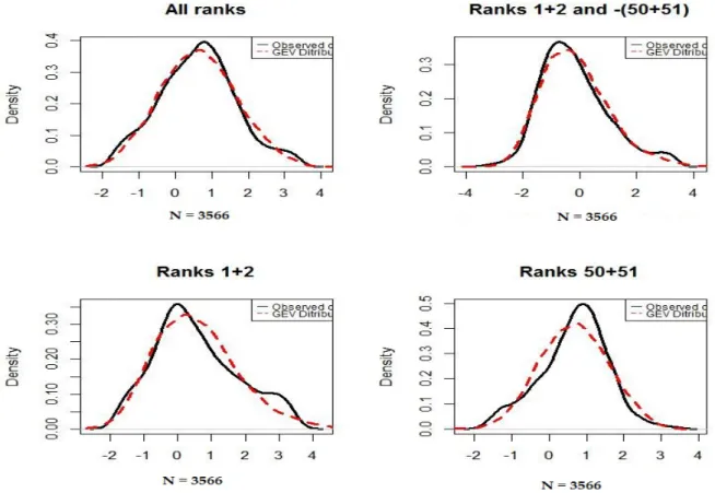
location, échelle). Nous allons choisir trois différents modèles de mélanges (par trois différents critères) et nous les utilisons pour produire des nouvelles prévisions, que nous allons du nouveau comparer aux prévisions initiales. Tous les trois modèles améliorent la compétence globale du SPE (CRPS), mais donnent un effet étrange au dernier rang de la queue droite du diagramme des rangs, effet confirmé par le calculs des quantiles (0.99, 0.98, 0.95) qui ne sont pas bien estimés par les prévisions données par nos modèles de mélange. Nous proposons de mettre en oeuvre une dernière méthode, en s’intéressant cette fois aux quantiles et non plus aux moments.
La méthode proposée est la méthode de régression des quantiles et elle fait l’objet de la troisième et dernière partie de thèse. Puisque nous voulons modéliser les queues, il est important de tenir compte des erreurs relatives aux quantiles. C’est pourquoi nous allons utiliser une distance de χ2 qui permet d’expliciter la sur-pondération des queues. Nous avons choisi les classes autour de la probabilité d’intérêt pour nous, soit 1 %: [0; 0, 01], [0, 01; 0, 02] et [0, 02; 0, 05] pour la partie inférieure de la queue et les classes symétriques pour la queue supérieure. Nous allons utiliser cette mesure pour estimer les améliorations apportées aux prévisions extrêmes. Les résultats sont positifs, même si il reste quelques biais dans la représentation de la queue.
Après avoir appliqué toutes ces méthodes, sur des données de températures de Météo France, sur une période de quatre ans nous sommes amenés à la conclusion que la meilleure méthode consiste à utiliser une méthode du type meilleur membre pour produire des simulations de tem-pérature pour le coeur de la distribution et d’adapter une régression quantile pour les queues de la distribution.
Summary
This work is carried out under a CIFRE thesis, as a partnership between the University of Paris Descartes (Laboratory MAP5) and the OSIRIS department of EDF R&D, France.
The thesis has for objective to study new statistical methods to correct temperature predictions that may be implemented on the ensemble prediction system (EPS) of Meteo France so to im-prove its use for the electric system management, at EDF France. The EPS of Meteo France we are working on contains 51 members (forecasts by time-step) and gives the temperature predic-tions for 14 days (also called time-horizons, 1 time-horizon = 24 hours) for the period: March 2007 - March 2011.
It is an univariate study: the 14 time-horizons will not be processed at the same time, the meth-ods will focus on one horizon at a time. Nevertheless we implement the chosen methmeth-ods for the ten horizons: from 5 to 14 independently. The time-horizons from 1 to 4 are not being integrated in our study because the deterministic forecasts are very good in this case of short time forecast. The thesis contains three parts: in the first one we present the EPS, then we present and im-plement two statistical methods supposed improving the accuracy or the spread of the EPS and we introduce criteria for comparing results. In the second part we introduce the Extreme Value Theory and the mixture models we use to combine the model we build in the first part with models for fitting the distributions tails. In the third part we introduce quantile regression as another way of studying the tails of the distribution.
Coming back to EPS, its principle is to run multiple scenarios of the same model with slightly different input data to simulate the uncertainty. This gives a probability distribution giving the probability of occurrence of a certain event. Ideally all the members of an EPS have the same probability to give the best prediction for a given time-step.
The methods we have evaluated are the method of the best member and the bayesian method. The forecasts obtained by the two methods when they are implemented to data from Meteo France are compared between them and then with the initial forecasts, through criteria of skill
and spread.
The method of the best member in its most complex variant is proposed by V. Fortin (see [FFS06]). The idea is to design for each time-step in the data set, the best member (we consider that a member is the best for a certain time-step when the prediction it gives has the smallest error, in absolute value, relative to the realization of the time-step.) among all scenarios (51 in our case) and to construct an error pattern using only the errors made by those best members and then to "dress" all members with this error pattern. This approach does not give good results in the case of the EPS that are already over dispersive. A second approach was developed to permit correction of this type of EPS. This approach proposes to "dress" ensemble members with different weights by class statistical ranks.
The bayesian method we introduce in the thesis is proposed by A. Raftery [RGBP04]. This is a statistical treatment of model output that provides calibrated probability distributions even if the initial EPS are not calibrated (we assume that a forecast is well calibrated when an event with a probability of occurrence of p occurs in average with a p frequency). With this method we compute the density function of the EPS as a weighted average of the densities of the com-ponents predictions scenarios. The weights are the probabilities of the scenarios of giving the best forecasts, estimated a posteriori and reflect the performance of each scenario, proven in a training period (the training period is a sliding window of a optimum length (found by certain criteria) that allows using a lighter database to estimate new parameters).
The predictions obtained by both methods are compared using criteria of skill and spread, spe-cific of the EPS as: the mean absolute error (MAE), the root mean square error (RMSE), the continuous rank probability score (CRPS), the Talagrand diagram, the reliability diagram. The bayesian method slightly improves the spread of the EPS for the bulk of the distribution but losses in overall skill of the EPS. The best member method does also improve the spread in its main mode and it also improve the overall skill from the CRPS point of view. These results make us want to study more in detail what happens in the tails of the distribution. Another possible continuation would have been the multidimensional forecasting (treating all time horizons simul-taneously). The need to manage the power system to measure and reduce the risk of failure makes us privilege the first track, the one concerning the study of the extreme values of the distribution. In the second part of the thesis we build a mixture model which allows us to use the best mem-ber method for the bulk of the distribution and a model specific to the extreme value theory for the tails. We first find a way for separating the distribution (find the tails heaviness), then we build the mixture model adequate to our needs. We also make some tests to find out if what we need to fit for the distributions tails is only one extreme model, or a combination of extreme models (function of time, tail, time-horizon). We choose three different mixtures models and we use them to produce new forecasts, which are compared to the initial forecasts. All the three models improve the global skill of the forecasting system (CRPS) but give a strange effect to the last rank of the right tail of the rank diagram confirmed by the quantile computations (.99,
.98, .95) that are not well estimated by the forecasts given by the mixture model. We propose to implement a last method, and this time we are not interest in moments, we are interested in quantiles.
The method is the quantile regression method and it is the subject of the third and last part of the thesis. Since we want to model the tails, it is important to take account the relative errors on quantiles. That is why we will use a χ2 distance which allows explicit over-weighting of the tails. We choose classes around the probability of interest for us, which is 1%: [0; 0.01], [0.01; 0.02] and [0.02; 0.05] for the lower tail, and the symmetric classes for the upper one. We will use this to measure all improvements and the results are positive even if there remains some biases in the tail representation.
In the end all the methods we implement on the ensemble prediction system for a four years period provided by Meteo France, when trying to improve its skill and/or spread bring us to the conclusion that the optimum method is to use a best member method type for the heart of the distribution and to adapt a quantile regression for the tails.
Publications and Conferences
Published Articles Gogonel A. Collet J. and Bar-Hen A., Statistical Post-processing Meth-ods Implemented on the Outputs of the Ensemble Prediction Systems of Temperature, for the French Electric System Management, is to be published in the Volume 5(2) of the Case Studies In Business, Industry And Government Statistics Journal, of the Bentley University, Massachusetts, USA.
Submitted Articles Gogonel A. Collet J. and Bar-Hen A., Improvement of Short-Term Ex-treme Temperature Density Forecasting using Best Member Method, is submitted at the Natural Hazards and Earth System Sciences Journal, published by the Copernicus GmbH (Copernicus Publications) on behalf of the European Geosciences Union (EGU).
Research Report Research Report Gogonel A., Collet J. et Bar-Hen A., Implementation of two methods of Ensemble Prediction Systems for electric system management, H-R32-2011-00797-EN, EDF R&D, May 2011
Conferences
1. 20th International Conference on Computational Statistics (COMPSTAT) 2012 Limassol (see [GAA12a]);
2. Workshop on Stochastic Weather Generators (SWGEN), Roscoff 2012 (see [GAA12b]); 3. International Conference of Young Scientists and Students (ICYSS-CS) , Sevastopol April
2012 (see [oYSS12]);
4. The World Statistics Congress (ISI), Dublin, Poster, August 2011 (see [GAAer]); 5. International Symposium on Forecasting, Prague, June 2011 (see [GAA11]);
6. 2ème Congrès de la Sociéte Marocaine de Mathématiques Appliquées, Rabat, Juin 2012 (see [GAA10]).
Chapter 1
Introduction
This first part of the thesis contains the presentation of the context where the need of this thesis appeared. It also contains the data we use to develop the methods we are proposing.
In this first part we are also presenting the Ensemble Prediction Systems, how and when they appeared, how they work and in what case they might be used. We use this first part to dedicate a few words to the uncertainty as this is "the reason" that makes important to have and to improve forecasts in meteorology or other domains.
We continue by presenting the two statistical methods supposed to improve the accuracy or the spread of the EPS and we introduce criteria for comparing results. The methods we have eval-uated are the method of the best member and the bayesian method. The forecasts obtained by the two methods when they are implemented to data from Meteo France are compared between them and then with the initial forecasts, through criteria of skill and spread of EPS as: the mean absolute error (MAE), the root mean square error (RMSE), the continuous rank probability score (CRPS), the Talagrand diagram, the reliability diagram.
The results we obtain will be presented in the next part of the thesis in the form of an article that is to be published in the Volume 5(2) of the Journal Case Studies In Business, Industry And Government Statistics, Bentley University, Massachusetts, USA.
1.1 Context and Data Description
1.1.1 Context
More and more users are interested in local weather predictions with uncertainty information, i.e. probabilistic forecasts. The energy sector is highly weather-dependent, hence it needs accurate forecasts to guarantee and optimize its activities. Predictions of the production are needed to optimize electricity trade and distribution. The needs in electricity depend on the meteorological conditions.
Electricité de France (EDF) is the most important electricity producer in France. The EDF R&D OSIRIS department is in charge of studying the management methods of the EDF-production system from a short time horizon (CT) to a medium time horizon (MT) (between 3 hours and 3 years, approximately). Short-term forecasting (that we will consider here) is important because the national grid requires a balance between the electricity produced and consumed at any moment in the day. In this department, the group Risk Factor, Price and Decisional Chain is in charge of studying and modeling the risk factors which can impact production system management. Among these risk factors, we shall be interested here in the physical risks [COL08]. Numerous specialists of the physics (for example the meteorologists) build sophisticated numer-ical models, with uncertainty on the input data. To take into account this uncertainty, they run the same model several times, with slight, but not random perturbation of the data. The prob-ability distributions obtained from the model is not a perfect representation of the risk factor, thus we need to implement statistical methods before we use it but when modeling the results we had to take into account that the results of physical models contain an irreplaceable information. The correlation between the temperature and the electricity consumption. Temperature is the main risk factor for an electricity producer such as EDF. Indeed, electric heating is well developed in France. If we take into account the variability of the temperature, the power consumed for the heating for a winter given-day may fluctuate about 20GW, that is 40 % of the average consumption. In what concerns the energy, the climatic risk factor is quantitatively less important, because the difference of energy consumed between the warmest and the coldest winters represents approximately 5 % of the energy over the year. Nevertheless, the climatic risk factor remains the first source of uncertainty for EDF. [CD10]
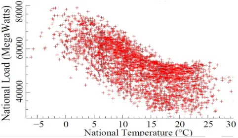
To explain the correlation between the temperature and the electricity consumption we can start by specifying that the French electrical load is very sensitive to temperature because the elec-trical heating development since the 70’s. The influence of the temperature on the French load is mostly known, except for the impact of air conditioning whose trend remains difficult to esti-mate . The electric heating serves to maintain a temperature close to 20°C inside the buildings. Taking into account that the "free" contributions of heat (sun, human heat), it is considered that the electric heating turns on approximately below 18°C. Beyond that temperature, the heat loss being proportional with the heat difference between inside and outside, the consumption
increases approximatively linearly. Besides, the buildings putting certain time to warm up or to cool down, the reaction to the outside temperature variations is delayed. In Figure 1.1 the non-linear relationship between electricity load and average national temperature at 9 AM (see [DOR09]).
Figure 1.1: Daily electricity loads versus the national average temperature from September 1, 1995 to August 31, 2004, at 9 AM.
This paper has for objective to study the ensemble prediction systems (EPS) provided by Meteo-France. We implement statistical post-processing methods to improve its use for electric system management, at EDF France.
Models used for load Forecasting at EDF are regression models based on past values of load, temperature, date and calendar events. The relationship of load to these variables is estimated by nonlinear regression, using a specifically preconditioned variant of S.G. Nash’s truncated Newton (see [NAS84]) developed by J.S. Roy. Load forecasting is performed by applying the estimated model to forecasted or simulated temperature values, date and calendar state. The short term forecasts are performed using an auto-regressive processes applied to the past two weeks residuals of the model (see [BDR05]). The model is based on a decomposition of the load into two components: the weather independent part of the load that embeds trend, seasonality and calendar effects and the weather dependent part of the load.
Up to the 4th time horizon the deterministic forecasts give high quality forecasts, this is why it continues to be used by Météo France for the wheatear forecasts up to four days ahead (see [ENM]). Starting from the 4th horizon, forecasts can be improved and/or the uncertainties in the forecasts better estimated. Currently the value used to predict the consumption is the mean
of the 51 forecasts.
Resorting to the EPS method allows on one hand to extend the horizon where we have good forecasts and on the other hand to give a measure of forecast uncertainty. Unlike the determin-istic solution the probability forecast is better adapted to the analysis of risk and decision-making. First, we study the Meteo-France temperature forecasts in retrospective mode and the temper-ature realizations in order to establish the statistical link between these two variables. Then, we examine two statistical processing methods of the pattern’s outputs. From the state of the art of the existing methods and from the results obtained by the verification of the probability forecasts, a post-processing module will be developed and tested. The goal is to achieve a robust method of statistical forecasts calibration. This method should thus take into account the un-certainties of the inputs (represented by the 51 different initial conditions added to the pattern). The first method is the best member method (BMM) and it is proposed by V. Fortin ([FFS06]) as an improvement of the one built by Roulston and Smith [RS02], and improved by Wang and Bishop [WB05]. The idea is to design for each lead time in the data set, the best forecast among all the k forecasts provided by the temperature prediction system, to construct an error pattern using only the errors made by those "best members" and then to "dress" all the members of the initial prediction system with this error pattern. This approach fails in cases where the initial prediction systems are already under (or over) dispersive because when an EPS is under dispersive, the outcome often lies outside the spread of the ensemble increasing the probability of the extreme forecast to give the best prediction. And the other way, when a ensemble is over dispersive the probability of the members close to the ensemble mean to be the best members is increasing. It is why a second method was created. It allows to "dress" and weight each member differently by classes of its statistical order.
The second method we implement is the bayesian method that has been proposed by A. Raftery ([RGBP04]). It is a statistical method for post processing model outputs which allows to provide calibrated and sharp predictive Probability Distribution Functions even if the output itself is not calibrated (forecasting are well calibrated if for a p probability forecasts, the predicted event is observed p times). The method allows to use a sliding-window training period (TP) to estimate new models parameters, instead of using all the database of past forecasts and observations. Results will be compared using standard scores verifying the skill and/or the spread of the EPS: MAE, RMSE, ignorance ccore, CRPS, Talagrand diagram, reliability diagram, bias, mean.
1.1.2 Data Description
We are working on the daily average temperatures in France from march 2007 to march 2011 and the predictions given by Meteo France for the same period. The temperature forecasts is provided by Meteo-France as an ensemble of temperatures prediction system containing the daily average temperatures in France (the weighted mean of 26 values of daily means temperatures
Figure 1.2: The map of the Meteo France stations.
observed by the Meteo stations in France, see Figure1.1.2) from March 2007 to March 2011 and the predictions given by Meteo France for the same period as an Ensemble Prediction System (EPS) containing 51 forecasts by day, up to 14 time-horizons, corresponding to 14 days.
The 51 members of the EPS are 51 equiprobable scenarios obtained by running the same forecast-ing model with slightly different initial conditions. Figure1.1.2represents for one fixed time-step the curves of the evolutions of the 51 scenarios by time-horizon, from 1 to 14. We can notice a small bias (∼ 0.1◦) starting with the first horizon. The bias is increasing with the horizon-time (normal) and that for all the scenarios in a resembling way.
We observe that the scenarios are randomly named by numbers from 0 to 50, which are not constant from one day to another. Hence, the uncertainty added to ensemble members is not related to the number of the ensemble member (the scenario 0 is the only one standing the same, as it is the one with no perturbation of the initial conditions added).
We start by making an univariate study i.e. we fix the horizon-time. Depending on the quality of the results we could consider a multivariate study.
éTherefore the horizon is fixed, we choose to study the forecasts starting with the 5th horizon because up to horizons 3-4 the determinist forecasts are very good (the Meteo-France pattern is
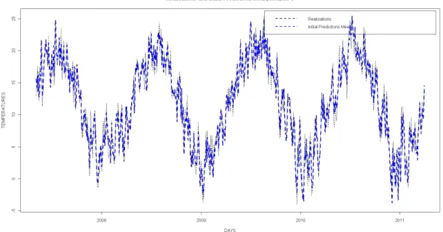
Average Forecast and Real Temperatures Curves
The evolution of the predictions by horizon from one to fourteen, for all scenarios
Figure 1.3: Figures corresponding to initial predictions. On top, the curve of realiza-tions and the one of the average predicted temperature. At the bottom, the curves of temperatures for one day, for all the 14 horizons time.
1.2 Ensemble prediction systems (EPS)
The ensemble prediction systems are a rather new tool in operational forecast which allows faster and scientifically justified comparisons of several forecast models. The EPS are built with the aim of obtaining the probability of the meteorological events and the zone of inherent uncertainty in every planned situation. It is a technique to predict the probability distribution of forecast states, given a probability distribution of random analysis error and model error.
The principle of the kind of EPS we are interested in, is to run several scenarios of the same model with slightly different input data in order to simulate the uncertainty (another way to simulate it would be by varying the physical models and/or its parametrization). Then we ob-tain a probability distribution function informing us about the probability of realization of a forecast. Ideally, the members of a EPS are independent and have the same probability to give the best forecast. Nevertheless, this information is not completely suited to the use for electric system management. For example, PDFs are not smooth, it is a major issue for uncertainties management.
At present, the EPS are based on the notion that forecast uncertainty is dominated by error or uncertainty in the initial conditions. This is consistent with studies that show that, when two operational forecasts differ, it is usually differences in the analysis rather than differences in model formulation that are critical to explaining this difference, see [DOC02].
Among the points of interest in using EPS ([MAL08]) is that it allows to estimate the uncertainty, to have a representative spread of the uncertainty that is in practice, to have an empirical standard deviation of the forecasts comparable with the standard deviation of the observations. EPS may also be used to give an estimation of the probability of occurrence of an event, it helps finding the threshold above (or beyond) which the risk of occurrence of the event is important.
1.2.1 History and building methods
The stochastic approaches in predicting weather and climate was seriously reconsidered after Lorentz discovered the chaotic nature of atmospheric behavior in the 1960s (see [BS07]). Ac-cording to him the atmosphere has a "sensitivity" in the initial conditions i.e. small differences in the initial state of the atmosphere could lead to large differences in the forecast.
In 1969, Epstein proposed a theoretical stochastic-dynamic approach to describe forecast error distributions in model equations. But the computing power at that time made his approach unrealistic [EPS69].
Instead, Leith proposed a more practical Monte-Carlo approach with limited forecast members. Each forecast member is initiated with randomly perturbed, slightly different initial condition
(IC). Leith showed that Monte-Carlo method is a practical approximation to Epstein’s stochastic-dynamical approach, [LEI74]. Leith’s Monte-Carlo approach is basically the traditional definition of ensemble forecasting although the content of this definition has been greatly expanded in the last 20 years [DU07].
As computing power increased, operational ensemble forecasting became a reality in early the 1990s. Both National Centers for Environmental Prediction in the USA (NCEP) and the Eu-ropean Center for Medium-Range Weather Forecast(ECMWF) operationally implemented their own global model-based, medium-range ensemble forecast systems. Hence the idea of this kind of prediction systems is to get an ensemble of forecasting models starting with just one model. There are different methods the prediction centers use to create an Ensemble Prediction System (EPS)(not to confound with the methods we will implement, which are post processing meth-ods, hence they are applied on EPS which have already been created). Among the most known methods used to create EPS, there are:
• Method of crossing (used in the USA, NCEP), see [SWa06].
• Method of the singular vector (used in Europe, ECMWF, see [DOC06]). • Kalman Filter (used in Canada), see [VER06].
The EPS we are using is built by the singular vector method, more exactly it is a ECMWF EPS which evolutions in time can be studied as in [MBPP96]. A description of the current operational version is given by Leutbecher and Palmer (see [MP07]). Since 12 September 2006, the ECMWF EPS has been running with 51 members one being the control forecast (starting from unperturbed initial conditions) and the other 50 are member to whom the initial conditions have been perturbed by adding small dynamically active perturbations (see [BBW+07]). These
51 runs are performed twice a day at initial time 00 and 12 UTC, up to 15 days-ahead, with a certain resolution from day 0 to 10 and a lower resolution for the days up to 15.
1.2.2 Forecasts and uncertainty in meteorology
Given the presence of errors at all levels of the forecasts building, the state of the atmosphere at some point is not perfectly known. This makes delicate to define a single "true" set of parameters. It is nevertheless possible to evaluate the probability of a set of parameters or data input. The uncertainty indicates the intrinsic difficulty in forecasting the event during a period. The best characterization of the uncertainty would be the probability density functions of the simulation errors. Computing a probability density function (PDF) for given model outputs (such as fore-cast error statistics) is in practice a difficult task primarily because of the computational costs [MAL05]. If we want to list some large classes of uncertainty that would be:
• Natural or fundamental uncertainty. It is the uncertainty of the probabilistic nature of the model. It is the uncertainty that remains when one has the right model and the right model parameters.
• The statistical uncertainty. The model parameters being estimated, there is certainly a bias between them and the "true" model parameters.
• The model uncertainty itself. Choosing a wrong law for as the distribution law. For example, suppose in a certain context that the population is normally distributed when in fact a gamma could be the "good" law to apply.
Sources of forecast errors
To be able to predict the forecast’s error, it is necessary to understand the most important components of this error. In order to find the step in the building process of the forecasting, creating errors Houtemaker ([HOU07]) made a list of the most important components of forecast error. There are some of those errors:
Incomplete observations of the atmosphere it is not possible to observe all variables at all locations and at all times.
Error in input data. The precision of the observations is sometimes limited. It can be a random error or a systematic one. Different observations taken by identical platforms can present correlated errors. Because of the observation error among others, the weather forecast will never be established from an perfect initial state.
Weighting observations. In the procedure of data assimilation, a weighted average is cal-culated from the new observations. The precision of the chosen weights is function of the relative precision of the observations.
Error due to the pattern. Because of the lack of resolution, the model shows a behavior a little bit different from the real behavior of the atmosphere in identical initial conditions.
1.3 The verification methods for EPS
Meteorologists have used EPS for several years now and in the same time many methods of evaluating their performances were also developed [SWB89]. A proper scoring rule maximizes the expected reward (or minimizes the expected penalty) for forecasting one’s true beliefs, thereby discouraging hedging or cheating (see [JS07]). One can distinguish two kind of methods: the ones permitting to evaluate the quality of the spread and the ones giving a score (a numerical result) permitting to evaluate the performance of the forecasts [PET08].
Hence, we need to verify skill or accuracy (how close the forecasts are to the observations) and spread or variability (how well the forecasts represent the uncertainty) (see [JS03]). If model errors played no role, and if initial uncertainties were fully included in the EPS initial pertur-bations, a small spread among the EPS members would be an indication of a very predictable situation i.e. whatever small errors there might be in the initial conditions, they would not seri-ously affect the deterministic forecast. By contrast, a large spread indicates a large uncertainty of the deterministic forecast (see [PER03]). As for the skill, it indicates the correspondence between a given probability, and the observed frequency of an event in the case this event is forecast with this probability. Statistical considerations suggest that even for a perfect ensemble (one in which all sources of forecast error are sampled correctly) there is no need to have a high correlation between spread and skill (see [WL98]).
1.3.1 Standard Statistical Measure
Let y be the vector of model outputs and let o be the vector of the corresponding observations. These vectors both have n components. Their means are y and o.
Bias
To study the (multiplicative) bias of the EPS is to study if the forecast mean is equal to the observed mean. Biasm = 1 n n X i=1 yi oi (1.1)
It is simple to use. It does not measure the magnitude of the errors and it does not measure the correspondence between forecasts and observations. The perfect score is 1 but it is possible to get a perfect score for a bad forecast if there are compensating errors.
Correlation coefficient
It measures the correspondence between forecasts and observations and is given by the variance between forecasts and observations (r2), a perfect correlation coefficient is 1.
r= Pn i=1(yi − y)(oi − o) pPn i=1(yi − y)2Pni=1(oi − o)2 (1.2)
Mean absolute error (MAE)
It measures overall accuracy and is defined as: M AE = 1 n n X i=1 |yi− oi| (1.3)
It is a linear score which provides the average amplitude of the errors without showing in what direction the errors are.
The root mean square error (RMSE).
A related error measure is the mean square error (MSE), defined as MSE = 1
N
PN
i=1(yi− oi)2
but one uses more its square root, RMSE as it has the advantage of being recorded in the same unit as the verifications. Like the MAE, it does not provide the direction of the errors but compared to the MAE puts greater influence on large errors than small errors in the average. If the RMSE is much greater than the MAE this would show a high error variance, the case of equality appears when all errors have the same magnitude. It can never be smaller than the MAE.
1.3.2 Reliability Criteria
The reliability (or spread) measures how well the predicted probability of an event correspond to its observed probability of occurrence. For a p probability forecast, the predicted event should be observed p times.
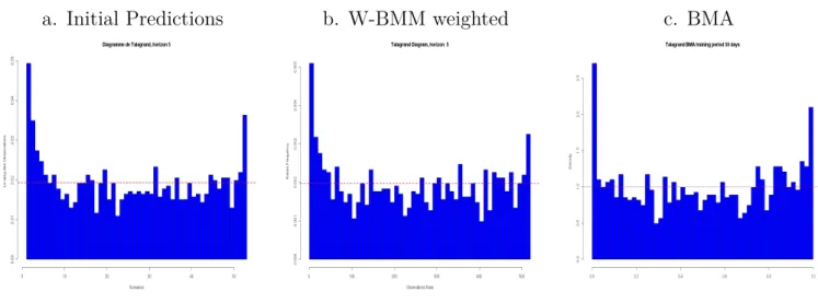
Talagrand diagram
The Talagrand diagram is a type of bar chart in which categories are represented by bars of varying ranks rather than specific values - a histogram of ranks. It measures how well the spread of the ensemble forecast represents the true variability (uncertainty) of the observations. For each time instant (day) we consider the ensemble of the forecasts values (the observation value included). The values within this ensemble are ordered and the position of the observation is noted (the rank). For example the rank will be 0 if the observation is below all the forecasts and N if the observation is above all the forecasts. Repeating the procedure for all the forecasts we obtain a histogram of observations rank. By examining the shape of the Talagrand diagram, we can draw conclusions on the bias of the overall system and the adequacy of its dispersion (see Figure 1.3.2):
• A flat histogram - ensemble spread correctly represents forecast uncertainty. It does not necessarily indicate a skilled forecast, it only measures whether the observed probability distribution is well represented by the ensemble.
• A U-shaped histogram - ensemble spread too small, many observations falling outside the extremes of the ensemble
Figure 1.4: Possible situations for the Talagrand Diagram
• A Dome-shaped - ensemble spread too large, too many observations falling near the center of the ensemble
• Asymmetric - ensemble contains bias.
Probability integral transform (PIT)
This method is the equivalent of the diagram of Talagrand for an ensemble having the shape of a probability density function (PDF). Let F be the the cumulative PDF, the value for the observation x(0) is simply F (x(0)), or a value between 0 and 1. By repeating the process for all the observations, we obtain a histogram having exactly the same characteristics as the diagram of Talagrand, as regards the performance of the ensemble [GRWG05].
Reliability Diagram
Reliability diagram is the plot of observed probability against forecast probability for all proba-bility categories. A good reliaproba-bility implies a curve close to diagonal. The deviation from diagonal shows a conditional bias, if it is below the diagonal then the probabilities are too high, if it is above diagonal then the probabilities are too low. A flatter curve shows a lower resolution. For a specific event the reliability diagram represents the frequency of occurrence of a probability
in the EPS and among the observations [POC10]. In this diagram, the forecast probability is plotted against the observed relative frequency.
1.3.3 Resolution (sharpness) Criteria
The resolution (or accuracy, or skill) is the measure of the ability of the forecasts. Brier Score
The Brier score measures the mean squared probability error (Brier 1950). It is useful for exploring dependence of probability forecasts on ensemble characteristics and is applied to a situation of two possible outcomes (dichotomous variables). Let pi the probability given by the
EPS that the event occurs at each lead time i and oithe probability observed (at every lead time
i) that the event occurs so oi= 1 or oi = 0. The perfect BS is 0.
BS= 1 N N X i=1 (pi− oi)2 (1.4)
Continuous Rank Probability Score (CRPS)
The CRPS measures the difference between the forecast and observed cumulative distribution functions (CDFs). The CRPS compares the full distribution with the observation, where both are represented as CDFs. If F is the CDF of the forecast distribution and x is the observation, the CRPS is defined as:
CRP S(F, x) =
Z +∞
−∞ [F (y) − 11y≥x]
2dy (1.5)
where 11y≥x denotes a step function along the real line that attains the value 1 if y ≥ x and the value 0 otherwise. In the case of probabilistic forecasts the CRPS is a probability-weighted average of all possible absolute differences between forecasts and observations. The CRPS tends to be increased by forecast bias and reduced by the effects of correlation between forecasts and observations (see [SDH+07]). One of the advantages is that it has the same units as the predicted
variable (so is comparable to the MAE) and does not depend on predefined classes. It is the generalization of the Brier score for the case of the continuous variables. The CRPS provides a diagnostic of the global skill of an EPS, the perfect CRPS is 0, a higher value of the CRPS indicates a lower skill of the EPS.
The CRPS can be decompose in: reliability and resolution terms obtained by the CRPS decom-position proposed by Hersbach ([GIL12]).
We can notice that if all the members of the EPS give all the same prediction, the CRPS is equal to the MAE (it is the case for deterministic forecasts).
Ignorance Score
The Ignorance Score is defined as the opposite of the logarithm of the probability density function f for the observation o [PET08]. Hence, for a single probability we have:
ign(f, o) = − log(f(o)) For the PDF of a normal law N (µ, σ2) th ignorance score is :
ign[N (µ, σ2), y] = 1
2ln(2πσ2) + (y − µ) 2 2σ2 The average ignorance is given by
IGN = 1 n n X i=1 ign[N (µ, σ2), o] (1.6) ROC Curve
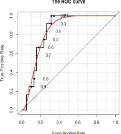
Probabilistic forecasts can be transformed into a categorical yes/no forecasts defined by some probability threshold. Hit rates H and false alarm rate F can be computed and entered into a ROC diagram with H defining the y-axis, F the x-axis (see Figure 1.3.3). The closer the F , H is to the upper left corner (low value of F and high of H) the higher the skill. A perfect forecast system would have all its points on the top left corner, with H = 100% and F = 0.
Figure 1.5: Each point on the ROC curve represents a sensitivity/specificity pair corre-sponding to a particular decision threshold.
1.4 Post-processing methods
1.4.1 The best member method
The best member method was proposed by V.Fortin [FFS06] and improves the studies previously led by Roulston and Smith [RS02] then by Wang and Bishop [WB05]. The idea is to design for each time-step in the data set, the best forecast among all scenarios (51 in our case) and to con-struct an error pattern using only the errors made by those "best members" and then to "dress" all members with this error pattern.
This approach fails in cases where the initial ensemble members are already under or over dis-persive, because when an EPS is under disdis-persive, the outcome often lies outside the spread of the ensemble increasing the probability of the extreme forecast to give the best prediction (conversely for over dispersive EPS). A possible solution is to "dress" and weight each mem-ber differently, using a different error distribution for each order statistic of the ensemble. So we can distinguish two more specialized methods: the one with constant dressing, or the un-weighted members method and the one with variable dressing, or the weighted members method.
The un-weighted members method
The temperature prediction system provides the forecasts xt,k,j, where k is the scenario’s number,
t is the time when the forecast is made and j is the time-horizon. The method is presented in univariate case so from the start j is fixed, hence xt,k,j becomes xt,k where we rename t as the
time for which the forecast is made.
Let yt be the unknown variable which is forecasted at the moment t, and let Xt = {xt,k, k =
1, 2, ..., K} be the set of all ensemble members of the forecasting system. Given Xt the purpose
is to obtain a probabilistic forecasts i.e. p(yt|Xt) in order to provide many more predictive
simulations p(yt|Xt) sampled from p(yt|Xt) where Xt= {xt,m, m= 1, 2, ..., M} with M K.
The concept of conditional probability allows to take into account in a forecast additional infor-mation (in this case it will be the forecasts given by Meteo France).
The basic idea of the method is to "dress" each ensemble member xt,k with a probability
distri-bution being the error made by this member when it happened to give the best forecast. The best scenario is defined x∗
t as the one minimizing kyt− xt,kk for a given norm k · k. As we are
working in an univariate space, the norm is the absolute value: x∗
t = argxt,kmin |yt− xt,k|
For an archive of past forecasts a probability distribution (pε∗) is created from the realizations
of ε∗ t = yt− x∗t: p(yt|Xt) ≈ 1 K K X k=1 pε∗(yt− xt,k) (1.7)
To dress each ensemble members one resamples from the archive of all best-member errors. Hence, the simulated forecasts are obtained by:
ˆyt,n= xt+ εt,n (1.8)
where εt,n is randomly drawn from the estimated probability distribution of ε∗t and n is the
number of simulations by time step.
This first sub-method where all the scenarios are ’dressed’ using the same distribution of the error is a choice adapted to the EPS where the scenarios have, a priori, the same probability to give the best forecast. When the initial EPS is already over dispersive, adding noise to each member will increase the variance of the new system.
The weighted members method
Fortin applied this method on a synthetic EPS1. He observed that this method failed in the
case of over dispersive or under dispersive EPS. The explanation is that when an EPS is under dispersive, the outcome often lies outside the spread of the ensemble. Hence, an extreme forecast has much more chances of giving the best prediction than a forecast close to the ensemble mean. Conversely, when a ensemble is over dispersive the members close to the ensemble mean have much more chances to be the best members than the extremes forecast. Hence, the probability that an ensemble member gives the best forecast as well as the error distribution of the best member are depending on the distance to the ensemble mean. For univariate forecasts we can sort the ensemble members by their distance to the best ensemble members and consider the rank of a member at the dressing sequence.
The only changes in second method, proposed for over (or under) dispersive systems, are the ones related to the use of the statistical rank:
Let
• xt,(k) be the kth member of the ensemble Xt= {xt,k, k = 1, 2, ..., K} ordered by statistic
rank. • ε∗
(k) = {yt− x∗t| x∗t = xt,(k), t= 1, 2, , ..., T } be the errors of the best ensemble members for
every t moment in a database of past forecasts, when the best forecast has the rank k. To dress each ensemble members differently, instead of resampling from the archive of all best member errors, one resamples from ε∗
(k) to obtain dressed ensemble members. Hence, the simu-lated forecasts are obtained:
ˆyt,k,n = xt,(k)+ ω · εt,(k),n (1.9)
1A synthetic EPS is an EPS built under certain conditions (ensemble members are independent and
identically distributed) and to whom we can vary the parameters we want in order to test different hypothesis or methods
where
• εt,(k),n drawn at random from ε∗(k) • ω =rs2
s2ε∗ and s2ε∗ =
1
T−1
PT
t=1(ε∗t,(k))2 is the estimated variance of the best-member error.
The parameter ω is greater than 1, in the case of the over dispersive forecasts and ω < 1 in the case of under dispersives systems.
1.4.2 Bayesian model averaging
The Bayesian approach is based on the fact that computing the probability of realization of an event does not depend only on its frequency of appearance but also on the knowledge and experience of the researcher. His judgment should naturally be coherent and reasonable. The Bayesian approach implies that two different points of view are not necessarily false, as in the principle of equifinality : the same final state can be reached from different initial states by different ways [BER72].
We base our study of the bayesian method, more exactly on the work of A.Raftery and T.Gneiting proposing bayesian model averaging (BMA) as a standard method which combine predictive distributions from different sources (see [RGBP04]). It is a statistical method for postprocessing model outputs which allows to provide calibrated and sharp PDFs even if the output itself is not calibrated. Raftery’s study is implemented on a 5 terms ensemble system coming from different, identifiable sources. It is specified that it is also applicable to the exchangeable situation, and the R-package ensembleBMA, by the same authors, is proving it by offering the choice of the exchangeability in its function definitions. But the second main difference between this study and ours is the significantly larger number of the ensemble members, so we expect to have much longer computation times.
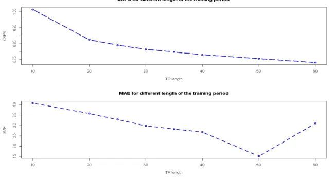
The original idea in this approach is to use a moving training period (sliding-window) to estimate new models parameters, instead of using all the database of past forecasts and observations. This implies the choice of length for this sliding-window training period and the principle guiding this choice is that probabilistic forecasting methods should be designed to maximize sharpness subject to calibration. It is an advantage to use a short training period in order to be able to adapt rapidly to changes (as weather patterns and model specification change over time) but the longer the training period, the better the BMA parameters are estimated [RGBP04]. After comparing training period lengths (from 10 to 60) by measurements as the RMSE, the MAE, the CRPS Raftery concludes that there are substantial gains in increasing the training period up to 25 days, and that beyond that there is little gain. The main difference between their case and ours is that they have 5 models and we have 51 (scenarios).
Let yT be the quantity to be forecasted and M
According to the law of total probability, the forecasts PDF, p(y) is given by: p(y) = XK
k=1
p(y|Mk)p(Mk) (1.10)
where p(y|Mk) is the forecast PDF based on Mk and p(Mk) is the posterior probability of model
Mk giving the best forecast computed on the training data and tells how the model is fitting
the training data. The sum of all k posterior probabilities corresponding to the k models is 1: PK
k=1p(Mk) = 1. This allows us to use them as weights, so to define the BMA PDF as a
weighted average of the conditional PDFs.
This approach uses the idea that there is a best "model" for each prediction ensemble but it is unknown. Let fk the bias-corrected forecast provided by Mk, giving the best prediction, to
which a conditional PDF gk(y|fk) is associated. The BMA predictive model will be:
p(y|f1, .., fk) = K
X
k=1
wkgk(y|fk) (1.11)
where wk is the posterior probability of forecast k being the best one and is based on forecast’s
kperformance in the training period. PKk=1wk= 1.
For temperature the conditional PDF can be fit reasonably well using a normal distribution centered at a bias-corrected forecast ak+ bkfk:, as shown by Raftery et al. (see [RGBP04]):
y|fk∼ N (ak+ bkfk, σ2)
The parameters ak, bkas well as the wk are to be estimated on the basis of the training data set:
akand bkby simple linear regression of yton fktfor the training data and wk, k= 1, .., K, and σ by
maximum likelihood (see [AF97]) from the training data. For algebraic simplicity and numerical stability reasons it is more convenient to maximize the logarithm of the likelihood function rather than the likelihood function itself and the expectation-maximization (EM) algorithm [DLR77] is used.
Finally the BMA PDF is a weighted sum of normal PDFs, the weights, wk, reflect the ensemble