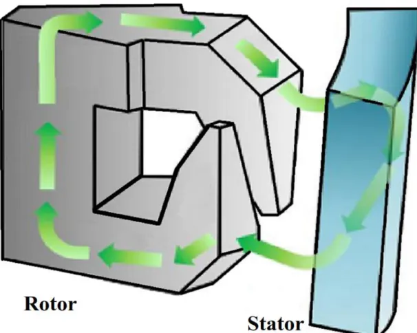
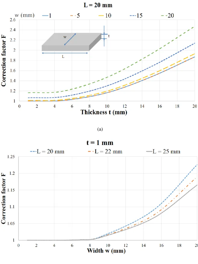
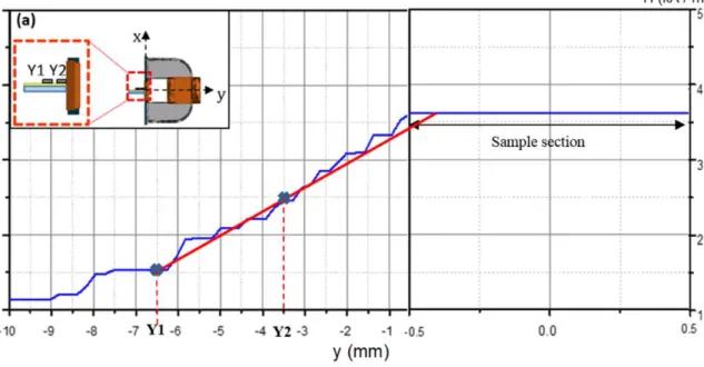
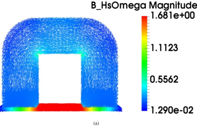
Development and validation of an electrical and magnetic characterization device for massive parallelepiped specimens

The parameters studied included bad level, amount of steel reinforcement, effective length of column, concrete strength, moisture Content, area and shape of cross

L’accès à ce site Web et l’utilisation de son contenu sont assujettis aux conditions présentées dans le site LISEZ CES CONDITIONS ATTENTIVEMENT AVANT D’UTILISER CE SITE WEB.

(The transition at TLow was not reported by them.) The small pressure dependence of TLow is in.. disagreement with the interpretation suggested

The microstructure and electrical properties of La 9.33 (SiO 4 ) 6 O 2 ceramic are investigated by X-ray diffraction (XRD), scanning electron microscopy (SEM) and

In this latter study, variance-component linkage analysis revealed weak evidence of linkage of KCNE1 SNPs with QTc interval while family-based association analysis

621-15 du Code monétaire et financier, s'applique seulement à la procédure de sanction ouverte par la notification de griefs par le collège de l'Autorité des

Dans les deux spécifications concernant les concours A du ministère des affaires étrangères, on trouve un écart de note à l’oral positif mais non significatif

Alors, la vie est un labyrinthe, on analyse, on avance comme dans le labyrinthe, il y a des choix à faire, des embranchement à prendre, on a souvent la carte de ses parents.. Mais