Energetic Macroscopic Representati on and Inversion Based Control of a Modular Multilevel Converter.

Science Arts & Métiers (SAM)

is an open access repository that collects the work of Arts et Métiers Institute of Technology researchers and makes it freely available over the web where possible.

This is an author-deposited version published in: https://sam.ensam.eu

Handle ID: .http://hdl.handle.net/10985/10045

To cite this version :

Philippe DELARUE, François GRUSON, Xavier GUILLAUD - Energetic Macroscopic Representati on and Inversion Based Control of a Modular Multilevel Converter. - In: Power Electronics and Applications (EPE), 2013 15th European Conference on, France, 2013-09-03 - Power Electronics and Applications (EPE), 2013 15th European Conference on - 2014

Any correspondence concerning this service should be sent to the repository Administrator : archiveouverte@ensam.eu

Energetic Macroscopic Representation and Inversion Based Control

of a Modular Multilevel Converter

P. Delarue

1

, F. Gruson

2

, X. Guillaud

3

1

_{L2EP, Lille 1 University, 59655 Villeneuve d’Ascq, France}

2

_{L2EP, Arts et Métiers ParisTech, 8Bd Louis XIV, 59046 Lille, France}

3

_{L2EP, Ecole Centrale de Lille, 59650 Villeneuve d’Ascq, France}

E-mail:

francois.gruson@ensam.eu

Keywords

«Multilevel converters», «Converter control», «FACTS», «Control methods for electrical systems», «Power transmission», «HVDC»

Abstract

This papers deals with the Modular Multilevel Converter (MMC). This structure is a real breakthrough which allows transmitting huge amount of power in DC link. In the last ten years, lots of papers have been written but most of them study some intuitive control algorithms. This paper proposes a formal analysis of MMC model which leads to the design of a control algorithm thanks to the inversion of the model. The Energetic Macroscopic Representation is used for achieving this goal. All the states variables are controlled to manage the energy of the system, avoid some instable operational points and determine clearly all the dynamics of the different loops of the system.

Introduction

The Modular Multilevel Converter is a power electronics structure which permits to reach high power and high voltage applications such as HVDC link or medium-voltage motor drives [1-6]. MMC presents lots of advantages: transformer less, modularity, high voltage quality, no high voltage DC bus, but also some drawbacks: difficulty to model [7] and to control due principally to high number of components [8].

The fig. 1 gives the structure of the converter. The three arms of this three-phased converter are composed of elementary modules. Each module is a simple switching cell. Depending on the state of the cell, the voltage of the capacitor is introduced or not in series with the main electrical circuit. Doing so, the voltage between the ‘+’ pole (or ‘-‘ pole) and a phase (1,2,3) may be modulated with a quasi sinusoidal shape. The discretization of the sinus is depending on the number of modules which can reach, for high power applications, several hundreds.

There exist many control structures for the MMC in the literature. Some of them are very simple but leads to non-sinusoidal output voltages and high voltage ripples on capacitor voltages [9] due to an important second harmonic component in arm currents. To improve voltage quality and reduce capacitor voltage ripples one can uses the CCSC (Circulating Current Suppression Controller) [10] or the control structures established in [9] or in [11]. These controls leads to satisfying characteristics in normal operation but it is difficult to predict the behavior in particular operating conditions such as unbalanced AC voltages. For example, Hagiwara and Akagi have been proved in [12] that the control presented in [11] can be unstable in certain conditions of operation and certain value of the controller parameters. This is the same problem as in the well known case of a buck converter with an L-C input filter and with constant output power [13].

Some of the controls presented in the literature have in common to be introducing by a heuristic way. One consequence is that these different controls have not the same number of controllers. But, to have a fully control of the energy stored in the system, the number of controllers must be equal to the number of independent state variables of the system. If not, some state variables may be out of control, can take unacceptable values and lead to unstable modes in particular operating conditions.

Other controls are inversion based controls which have been developed by a global inversion of the model and a feed-forward action to correct the error of the model. In this case, the global control can

ensure an efficient behavior of the entire system, but without taking into account energetic properties or behavior of each device [14], that can lead to common misconception [15]. Moreover these type of control structure leads to an important computation time.

E

module

DC side AC side v1, v2, v3 + -1 2 3

Fig.1: Circuit configuration of the MMC

To solve this problem the paper proposes to represent and control the MMC by the use of the Energetic Macroscopic Representation (EMR) [16]. EMR is a graphical description exclusively based on physical causality (i.e. integral causality), it highlights energy properties of the power components such as energy storage, energy conversion and energy distribution. Moreover, an inversion-based control can be systematically deduced, step-by-step, by inverting each element of the EMR [17]. Then, the control structure is not obtained “heuristically” but results from inversion rules application. The obtained control structure is composed of cascaded loops which ensure a physical and efficient energy management of each device. This inversion based control leads to have as many controllers as state variables in the system which thus increases the robustness of the system [18]. All the state variables are under control, which ensures all the dynamic of the system to be clearly defined in respect with a appropriate behavior of this type of system.

Modeling of the MMC

The study of MMC can be simplified by decoupling the problem of capacitor voltage balancing inside each arm and the problem of global control (currents and output power control). This decoupling has been first proposed in [9] and is now currently used. If the balancing is well done (uc1=uc2=…=ucn)

each arm is equivalent to a capacitor of C/N capacitance with a voltage uctot=uc1+uc2+…+ucN and an

ideal dc/dc converter controlled by its duty cycle as show in Fig. 2. So v=m.uctot and ic=m.i with

m=n/N where n corresponds to the number of active cells. Moreover, if N is great, m can be

assimilated to the value _α of the duty cycle so v=_α.uctot and ic=α.i. The voltage balancing system can

be done by using the cells with most charged capacitors when arm current is negative (to decrease voltage capacitor of the active cells) and using the cells with lower charged capacitors when arm current is positive (to increase voltage capacitor of the active cells). In this paper, we consider that the balancing system works properly and we focus the study on the global control of the structure.

Each arm of the MMC structure (Fig. 1) is aggregated in the proposed equivalent structure (Fig. 3). Using the Kirchhoff laws leads to 11 independent differential equations. The system is then characterized by 11 independent state variables: the six voltages across the 6 equivalent capacitors and

5 currents (for example three arm currents and two phase currents, the other currents are linear dependant of the 5 chosen currents).

Fig.2: Equivalent arm circuit configuration ie C/N C/N C/N C/N C/N C/N E DC side AC side v1, v2, v3 u_u1 i_u1 i_l1 u_l1 u_cu1 u_cl1 αu1 αl1 αu2 α u3 αl3 αl2 u_cu2 ucu3 u_cl2 ucl3 i_u2 i_u3 i_{l2 i} l3 L, R L’, R’ L’, R’ L’, R’ L’, R’ L’, R’ L’, R’ i_v1 i_v2 i_v3 u_u2 u_l2 u_u3 u_l3

Fig.3: Equivalent circuit configuration of the MMC

To reduce the ripple voltage across the equivalent capacitors, arm currents should be composed of a continuous component (equal to 1/3 of the DC current in the DC voltage source) and a sinusoidal component (equal to ½ of the corresponding phase current). It is by the control that these objectives will be achieved. In this purpose, the modeling is oriented by performing the now classic following change of variables:

{

1,2,3

}

2 2 2 ∈ + = − = + =i i e u u u u u i i li ui i diff i u i l i v i l i u i diff (1)

The system then can be split in two sub-systems as shown, for one leg, in Fig. 4 and then equations can be deduced:

when voltage balancing is efficient : N n i dt duc N C and N n uc v tot tot / = . / = v i uc_to n

/N =m

C/

Active cell number Total cell number

v i uc uc uc uc C C C C uc N uc uc uc uctot= 1+ 2+...+ N = . t

0

1

m

α

t withou t

α

m

0

1

with PW

For each of the three phase ⎪ ⎪ ⎩ ⎪⎪ ⎨ ⎧ + = − + + + = − − i diff i diff i diff i v i v no i i v i R dt di L u E i R R dt di L L v v e 2 ) 2 ' ( ) 2 ' ( (2) (3)

The 3 equations (2) are not independent because iv1+iv2+iv3=0. The application of Park transformation gives the following relationships (4) which replace the equations (2):

⎪ ⎪ ⎩ ⎪⎪ ⎨ ⎧ + − + + + = − + + + + + = − − − − − − − − − d v q v q v q q v q v d v d v d d v i L L i R R dt di L L v e i L L i R R dt di L L v e ω ω ) 2 ' ( ) 2 ' ( ) 2 ' ( ) 2 ' ( ) 2 ' ( ) 2 ' ( (4)

and for each of the six equivalent converters and capacitors

⎪⎩ ⎪ ⎨ ⎧ = = = = = = dt du N C i i dt du N C i i u u u u i cu i cu i u i u i cl i cl i l i l i cu i u i u i cl i l i l α α α α ₍₅₎ (6)

We can count 11 independent differential equations: 6 for the six voltages across the 6 equivalent capacitors (6), 3 for the 3 differential currents (3) and 2 for line currents in dq frame (4)

iu C/N C/N il iv uu ul ucu vr ucl E/2 E/2 vno L’,R’ L,R αu αl C/N C/N uu ul ucu ucl E/2 E/2 _L’,R’ α u αl vr vno L,R L’,R’ L’,R’ ev ½ i_v ½ i_v i_diff i_diff i_v

Fig.4: Arm decomposition

The 11 state variables are: the 5 current variables (idiff1, idiff2, idiff3, ivd and ivq) + the 6 voltage variables

(ucl1, ucl2, ucl3, ucu1, ucu2, ucu3)

The control aims to have three phase balanced sinusoidal currents iv1, iv2, iv3 (so constant ivd an ivq

currents) to obtain a given value of active and reactive power at the AC side. A constraint for the control is to have, in steady state, continuous differential currents idiff1, idiff2 et idiff3 and constant

equivalent capacitor voltage (ucl1, ucl2, ucl3, ucu1, ucu2, ucu3), in average value.

EMR of the MMC

Each equation is translated into EMR elements (see appendix for the summary table of EMR elements) and their inputs and outputs are defined according to the causality principle (i.e. integral causality). Moreover, connection between elements has to respect the interaction principle. The global EMR is depicted in the upper part (green or orange symbols) of Fig. 5. For the sake of clarity, all quantities are expressed in terms of vectors. The numbers in purple remind, in the EMR, the dimensions of the vectors. The numbers in parenthesis remind the corresponding equations.

Eq.(3) // coupling idiff DC Bus E i_dc E i_v AC Grid v_r-dq e_v i_diff u’_diff v_r i_v-dq iul icul uul ucul 6 e_dq i_v-dq i_v ucul P_{_ref} i_diff-ref P_{_ref} e_v E X 3 Q_{_ref} uc_ref 6 6 3 3 2 3 1 2 1 2 3 3 3 No overmodulation iv-0=0 0 2*Uc-ref P_ref uc_ref ev iv 2 v v e e /ˆ (Park) (Park-1₎ Eq.(5) Eq.(4) Eq.(1) Eq.(6)

iv-ref ivdq-ref edq-ref ev-ref

u’_diff-ref u_ul-ref

α

ul-ref iul-ref i_diff (Park)

Fig.5: EMR and Inversion Based Control of the MMC

One can see that there are 11 accumulation elements (6 for the six equivalent capacitors, 2 for the two equivalent line inductances, 3 for the 3 equivalent arm inductances) which leads to 11 state variables of the system.

Inversion Based Control of MMC

To develop the control algorithm, the inversion-based control rules of the EMR are used [17]. The control scheme is deduced from a step-by-step inversion of the model. First of all, the tuning paths have to be defined. These causal paths link the tuning inputs to the variables to be controlled. The tuning paths are represented on Fig. 5 by the big blue arrows.

To obtain the control structure all the elements along the tuning path are inverted. The inversion is direct when the elements contain no time dependent relationship (conversion elements or coupling elements). When elements contain integral relationships (accumulation elements), it cannot be possible to invert directly them to avoid derivative relationships. Their inversions are thus indirectly made using a controller and measurements.

The lower part of Fig. 5 (blue symbols) shows the deduced control structure (blue elements). The dark blue element is a strategy element which defines phase current references from P and Q references and from measured grid voltages. Note that the control part framed in dark blue is not the simple inversion of the corresponding system part (Eq. 5 and 6). Indeed the conservation of instantaneous power through the 6 equivalent converters constrains us to control equivalent capacitor voltages only in average value. So the inversion of equations (5) and (6) must be based on the conservation of power which can be written as follow:

⎪ ⎪ ⎩ ⎪⎪ ⎨ ⎧ + − − + = = + − − = = ) 2 )( 2 ( ) 2 )( 2 ( i diff i v i diff i v i l i l i cl i cl i diff i v i diff i v i u i u i cu i cu i i u e E i u i u i i u e E i u i u (7)

Integration, on a grid period T, of equations (7) leads to:

[

]

[

]

⎪ ⎪ ⎩ ⎪ ⎪ ⎨ ⎧ − = ⎟ ⎠ ⎞ ⎜ ⎝ ⎛ = − − = ⎟ ⎠ ⎞ ⎜ ⎝ ⎛ = − − − 2 . 2 ) 0 ( ) ( 2 1 2 . 2 ) 0 ( ) ( 2 1 2 2 2 2 AC DC i diff T cl i cl i cl AC DC i diff T cu i cu i cu P i E dt dW u T u N C T P i E dt dW u T u N C T (8)

where PAC is the active power on AC side. These relations shows that the differential currents

influence ucu i AND ucl i. So we have, by arm, only one variable (idiff i) to control two voltages (ucu i and

ucl i). One solution consists to merge the differential current idiff i into a DC component and an AC

component as illustrated on fig.6 and by relation (9).

AC i diff DC i diff i diff

i

i

i

₌

₋

₊

₋ (9)

idiff i_DC are supposed constant on a whole grid period T

idiff i_AC will be three phase sinusoidal components in phase with the ev i voltages

ucu_tot ucl_tot iu C/N C/N il uu ul L’,R’ αu αl ½ i_AC ½ i_AC i_diff-DC i_diff-AC i_diff

Fig.6: Decomposition of the differential current Equations (8) can then be rewritten as follow:

⎪ ⎪ ⎩ ⎪ ⎪ ⎨ ⎧ + − = ⎟⎟ ⎠ ⎞ ⎜⎜ ⎝ ⎛ − − = ⎟⎟ ⎠ ⎞ ⎜⎜ ⎝ ⎛ − − − − 2 ˆ ˆ 2 . 2 2 ˆ ˆ 2 . 2 AC i diff i v i ACph DC i diff T i cl AC i diff i v i ACph DC i diff T i cu i e P i E dt dW i e P i E dt dW (10)

where PACph i is the active power of the phase i. We can see that, by arm, idiff-DC will control the

capacitor voltage sum ucu+ucl while idiff-AC will control the capacitor voltage difference ucl-ucu:

⎪ ⎪ ⎩ ⎪ ⎪ ⎨ ⎧ = ⎟⎟ ⎠ ⎞ ⎜⎜ ⎝ ⎛ − − = ⎟⎟ ⎠ ⎞ ⎜⎜ ⎝ ⎛ + − − AC i diff i v T i cu i cl i ACph DC i diff T i cu i cl i e dt W W d P i E dt W W d ˆ ˆ ) ( . ) ( (11)

Because the equivalent capacitor voltages uculi will be constant in steady state, controlling stored

energy (Wcli, Wcui) or controlling equivalent capacitor voltages is almost the same. Then the figure 7

gives the inversion of equation (11) which corresponds to the dark blue framed part of fig.3. On this figure, Pref is the reference for AC side active power used in place of PAC measurement.

e

_v

i

_diff-DC

P

_{_ref}

E

X

2

ˆ

/

e

v

i

_diff-AC 6 3 3 ₃ 3 3 3

2*U

_c-ref

u

_cul

u

cu

+u

cl

u

_cu

-u

_cl

0

i

_diff-ref

i

_ul-ref

i

_v Fig.7: Inversion Based Control of equivalent converters and capacitors

It can be seen than the control structure (the bottom part of fig.3) contain 11 controllers (the same number than the independent state variables). So it is possible to tune the controllers (PI controllers are chosen for this work) to have a stable behavior whatever the operating point.

Simulation results

This control strategy has been implemented in Matlab-Simulink® software. The simulation results are given for a 1000MVA MMC converter. The chosen MMC components and the controllers’ time constant are presented in table. 1.

L 60 mH C/N 25 µF R 60 mΩ E 640 kV L’ 50 mH ω 314 rad.s-1 R’ 50 mΩ Vr 192 kV Tiv 10ms Tucu+ucl 50ms Tidiff 20ms Tucu-ucl 100ms

Table.1: Parameters of the studied MMC topology

Tiv is the time constant of the AC current, Tidiff for the differential current, Tucu+ucl for the capacitor

voltage sum and Tucu-ucl for the capacitor voltage difference.

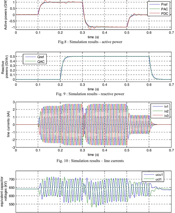
Figure 8 shows the active power PDC for the DC side, PAC for the AC side and its reference Pref (=0

until 0.1s, then =1GW until 0.3s, then =-1GW until 0.5s and finally =0). Figure 9 shows the reactive power Q and its reference Qref (=0 until 0.2s then =500MVAR until 0.6s and finally =0).

Figure 10 shows the three phase currents (iv1,iv2,iv3) which are sinusoidal as expected.

Figure 11 shows the equivalent capacitor voltages (ucl1, ucu1) in one converter arm. These voltages are

controlled in average value (here we have chosen uc-ref=E). Figure 12 shows arm currents (iu, il). The iu

and il currents are composed of a DC component and a sinusoidal component as expected (without

second harmonics).

Note that this results can’t be obtain in the same conditions (parameters of the system and dynamics of the control) with classical control structure described in the introduction without reducing power references to avoid instability or divergence of equivalent voltage capacitors.

0 0.1 0.2 0.3 0.4 0.5 0.6 0.7 -1 -0.5 0 0.5 1 time (s) A ct iv e pow er s ( G W ) Pref PAC PDC

Fig.8 : Simulation results - active power

0 0.1 0.2 0.3 0.4 0.5 0.6 0.7 0 0.1 0.2 0.3 0.4 0.5 time (s) Re a c ti v e p o w e rs (G V A r) Qref QAC

Fig. 9 : Simulation results - reactive power

0 0.1 0.2 0.3 0.4 0.5 0.6 0.7 -3 -2 -1 0 1 2 3 time (s) li n e c u rre n ts (k A ) iv1 iv2 iv3

Fig. 10 : Simulation results – line currents

0 0.1 0.2 0.3 0.4 0.5 0.6 0.7 550 600 650 700 time (s) eq ui v a lent c a p a c it o r v o lt ag es ( k V ) ucu1 ucl1

Fig. 11 : Simulation results – upper and lower equivalent capacitor voltages of one arm

0 0.1 0.2 0.3 0.4 0.5 0.6 0.7 -1.5 1 -0.5 0 0.5 1 1.5 time (s) a rm c u rre n ts (k A ) iu1 il1

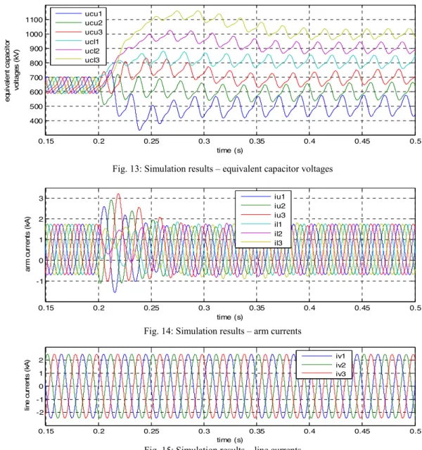
To illustrate the powerful of the proposed control the figure 13 gives the 6 equivalent capacitor voltages with different reference values (than E=640kV) imposed at 0.2s:

ucu1-ref=500kV , ucu2-ref=600kV , ucu3-ref=700kV , ucl1-ref=800kV , ucl2-ref=900kV , ucl3-ref=1000kV

After a short transient, capacitor voltages are controlled in average value to its reference values without effects on the arm currents (Fig.14) and on the AC currents (Fig.15). The interest to control capacitor voltages at different values will be exploited in future works.

0.15 0.2 0.25 0.3 0.35 0.4 0.45 0.5 400 500 600 700 800 900 1000 1100 time (s) e q ui v a le nt c a p a c it o r v o lt age s ( kV) ucu1 ucu2 ucu3 ucl1 ucl2 ucl3

Fig. 13: Simulation results – equivalent capacitor voltages

0.15 0.2 0.25 0.3 0.35 0.4 0.45 0.5 -1 0 1 2 3 time (s) a rm c u rr e n ts (k A ) iu1 iu2 iu3 il1 il2 il3

Fig. 14: Simulation results – arm currents

0.15 0.2 0.25 0.3 0.35 0.4 0.45 0.5 -2 -1 0 1 2 time (s) lin e c u rr e n ts (k A ) iv1 iv2 iv3

Fig. 15: Simulation results – line currents

Conclusion

The use of Energetic Macroscopic Representation (EMR) permits the modeling of the MMC and highlights the important couplings which exist between the different parts of the system.

The inversion of the model leads to a general architecture of the control which cope with all these couplings. The control architecture leads to have as many controllers as state variables in the system which thus increases the robustness of the system. All the state variables are under control, which ensures all the dynamic of the system.

With this solution it is possible to control individually each equivalent capacitor voltage without influences on line currents and power exchanges between the DC side and the AC side. This possibility will be used in the future to optimize the global behavior of the converter in some particular cases such as unbalanced grid voltages.

The general dynamic of this complex system may be correctly defined. This is very important for a future massive integration of these kind of converter in an AC system, which is it self a very large and complex dynamic system. The knowledge and control of the overall dynamic may also be important for the development of future multiterminal DC grids.

References

[1] R. Marquardt and A. Lesnicar, “A new modular voltage source inverter topology,” presented at the Rec. Eur. Conf. Power Electr. Appl. [CDROM], Toulouse, France, 2003.

[2] M. Glinka, “Prototype of multiphase modular-multilevel-converter with 2 MW power rating and 17-level-output-voltage,” in Proc. Rec. IEEE Power Electron. Specialists Conf. (PESC), 2004, pp. 2572–2576. [3] M. Glinka and R. Marquardt, “A new ac/ac multilevel converter family,” IEEE Trans. Ind. Electron., vol.

52, no. 3, pp. 662–669, Jun. 2005.

[4] M. Hagiwara, K. Nishimura, and H. Akagi, “A medium-voltage motor drive with a modular multilevel PWM inverter,” IEEE Trans. Power Electron., vol. 25, no. 7, pp. 1786–1799, Jul. 2010.

[5] Glinka. M. and Marquardt R.: A new AC/AC multilevel converter family, IEEE Transactions on IndustrialElectronics, Vol. 52 no 3, June 2005

[6] H. Akagi, “Classification, terminology, and application of the modular multilevel cascade converter (MMCC),” presented at the Rec. IPECSapporo, Japan, 2010

[7] Cherix N., Vasiladiotis M., Rufer A.: Functional Modeling and Energetic Macroscopic Representation of Modular Multilevel Converters, 15th International Power Electronics and Motion Control Conference, EPE-PEMC 2012 ECCE Europe, Novi Sad, Serbia

[8] Saad. H., Dennetiere. S, Mahseredjian. J, Nguefeu. S. : Detailed and Averaged Models for a 401-Level MMC–HVDC System, IEEE Transactions on Power Delivery, Vol. 27 no 3, July 2012, pp. 1501-1508 [9] A. Antonopoulos, L. Angquist, and H. P. Nee, “On dynamics and voltage control of the modular multilevel

converter,” in Conf. Rec. EPE [CD-ROM] Barcelona, 2009, pp. 1–10.

[10] Zheng Xu and Jing Zhang : Circulating current suppressing controller in modular multilevel converter, IECON 2010 - 36th Annual Conference on IEEE Industrial Electronics Society, 7-10 Nov. 2010, pp. 3198 - 3202

[11] Hagiwara M. and Akagi H.: “Control and Experiment of PWM Modular Multilevel Converters”, IEEE Transactions on Power Electronics, Vol. 24 no 7, pp. 1737-1746, July 2009

[12] Hagiwara M., Akagi.H : “Control and Analysis of the Modular Multilevel Cascade Converter Based on Double-StarChopper-Cells (MMCC-DSCC)”, IEEE Transactions on Power Electronics, Vol. 26, no 6, pp. 1649-1658, June 2011

[13] R.D. Middlebrook, “Input filter considerations in design and application of switching regulators”, IEEE Industry Applications annual meeting, 1976

[14] W. S. Lewine, “Input-Output model”, The Control Handbook, Chap. 5, pp. 65-72, CRC Press, 1996. [15] F. E. Cellier, H. Elmquist, M. Otter, “Modelling from physical principle”, The Control Handbook, Chap. 7,

pp. 99-108, CRC Press, 1996.

[16] K. Chen, A. Bouscayrol, A. Berthon, P. Delarue, D. Hissel, R. Trigui, “Global modeling of different vehicles, using Energetic Macroscopic Representation to focus on system functions and system energy properties”, IEEE Vehicular Technology Magazine, vol. 4, no. 2, June 2009, pp. 80-89

[17] P. J. Barrre, A. Bouscayrol, P. Delarue, E. Dumetz, F. Giraud, J. P. Hautier, X. Kestelyn, B. Lemaire-Semail, E. Lemaire-Semail, "Inversion-based control of electromechanical systems using causal graphical descriptions”, IEEE-IECON'06, Paris, November 2006.

[18] M. E. Sezer, “Decentralized control”, The Control Handbook, Chap. 49, pp. 779-793, CRC Press, 1996.

Appendix:

Synoptic of Energetic Macroscopic Representation (EMR) Source of energy Electrical converter (without energy accumulation) Element with energy accumulation

Example of coupling device (energy distribution) Control block without controller Control block with controller

Inversion of coupling device (with distribution input)