Experimental External Force Estimation Using a Non-Linear Observer for 6 axes Flexible-Joint Industrial Manipulators

Science Arts & Métiers (SAM)

is an open access repository that collects the work of Arts et Métiers Institute of

Technology researchers and makes it freely available over the web where possible.

This is an author-deposited version published in: https://sam.ensam.eu

Handle ID: .http://hdl.handle.net/10985/8178

To cite this version :

Jinna QIN, François LEONARD, Gabriel ABBA - Experimental External Force Estimation Using a Non-Linear Observer for 6 axes Flexible-Joint Industrial Manipulators - In: 9th Asian Control Conference, ASCC 2013; Istanbul; Turkey, Turkey, 2013-06-23 - 9th Asian Control Conference, ASCC 2013; Istanbul; Turkey - 2013

Any correspondence concerning this service should be sent to the repository Administrator : archiveouverte@ensam.eu

Experimental External Force Estimation Using a

Non-Linear Observer for 6 axes Flexible-Joint

Industrial Manipulators

Jinna Qin

Design, Manufacturing and Control Laboratory (LCFC)

Arts et M´etiers ParisTech 57078 Metz, France Email: jinna.qin@ensam.eu

Francois L´eonard

Design, Manufacturing and Control Laboratory (LCFC) National Engineering College of Metz

57035 Metz Cedex, France Email: leonard@enim.fr

Gabriel Abba

Design, Manufacturing and Control Laboratory (LCFC)

Arts et M´etiers ParisTech 57078 Metz, France Email: gabriel.abba@ensam.eu

Abstract—This paper proposes a non-linear observer to

es-timate not only the state (position and velocity) of links but also the external forces exerted by the robot during Friction Stir Welding (FSW) processes. The difficulty of performing this process with a robot lies in its lack of rigidity. In order to ensure a better tracking performance, the data such as real positions, velocities of links and external forces are required. However, those variations are not always measured in most industrial robots. Therefore, in this study, an observer is proposed to reconstruct those necessary parameters by using only measurements of motor side. The proposed observer is carried out on a 6 DOF flexible-joint industrial manipulator used in a FSW process.

I. INTRODUCTION

A. Robot and control

Current studies propose to replace some special machine-tools by industrial robots because of their effective cost and larger workspace compared with usual machine-tools. The technical and economic performances of production can be greatly improved by using a manipulator or a robotic system as a tool holder. However, performance issue is one of the reasons that prevent robotization of industrial manufacturing. Moreover, in industrial production, it is very difficult to change the mechanical elements or the inner robot control system. This study concerns an industrial manipulator KUKA KR500 MT-2, which has a payload of 500 kg and can be used for a FSW process [1], [2] where a very significant interaction force is required. Up to now, this process is usually carried out by some specially developed machines, having strongly rigid axes but more expensive. The objective of this work is to realize the required process with a 6 DOF serial chain industrial manipulator.

The concerned robot only has motor side measurements: the angular positions θ and speeds ˙θ as well as the currents

of actuators. Due to flexibility of the transmission chain, the state of links cannot be deduced from the one of motor side. In order to facilitate the realization of these operations, the state of links (q, ˙q) and the external torque applied on the tool

is required to be known. Either the components of the torque are difficult to measure or the sensor required for high forces of FSW is expensive. One solution is to use an observer to estimate those essential parameters [3].

An extended state observer (ESO) is proposed for the state feedback control of a flexible joint robotic system in [4]. This approach is used for state estimation, which is then validated with a Quanser’s flexible-joint module. An acceleration-based observer is presented in [5] for state obser-vation with an experimental validation. However, this observer needs measurement of link accelerations, which are generally not measured by industrial robots. [6] investigates methods for tool position estimation of industrial robots, which also requires tool acceleration measurement. An application of disturbance observers to non-linear systems is given in [7] and an observer-based adaptive robust control (ARC) approach for FSW process is discussed in [8] proving that axial force can also be estimated by an observer, however, these approaches do not consider flexibility of joints. Unique Lyapunov-based non-linear observer is difficult to apply systematically [9]. Disturbance observer technique is widely used in mechanical servo systems, and a disturbance dual observer based control algorithm is proposed for industrial robots having flexible joints in [10], which can use state of motor to construct state of link as well as disturbances. Nevertheless, in this paper the observer is under the assumption that the disturbance dynamics are known and proportional to the error of estimation.

B. Contributions and outline of the paper

The contribution of this paper is mainly about the extension of the observer proposed by [11] to cover estimation of external forces applied by the robot by using only position, velocity and current measurements of motor axes. This paper describes an improved observer of our previous work in [12]. This observer is adapted for a 6 DOF flexible robot system, and modified to deal with variable external forces. Simulations and experiments show that the new proposed observer has much better performance than the one we proposed before. With the new observer, significant and variable external forces can be well estimated for industrial robots. Moreover, in this paper, a complete flexible-mode manipulator model of robot KUKA KR500 MT-2 is described.

The modeling of robot and process are presented in Section II. The design of our new observer is described in Section III. In Section IV results of experiments with robot KUKA KR500

Fig. 1. Robot KUKA KR500 MT-2 (by courtesy of Institut de Soudure) TABLE I. MDHPARAMETERS OF ROBOTKUKA KR500 MT-2.

j µj σj αj dj θj rj 1 1 0 π 0 q1 −L1z 2 1 0 π/2 L1x q2 0 3 1 0 0 L2 π/2 + q3 0 4 1 0 −π/2 D4 q4 −L34 5 1 0 π/2 0 q5 0 6 1 0 −π/2 0 −π/2 + q6 −L5 7 0 2 0 0 0 −Ltz

MT-2 are provided. These results showed good performances of the proposed observer. Finally, conclusions and directions for future work are discussed in Section V .

II. MODELING OF FLEXIBLE JOINT ROBOT AND FSW PROCESS

The robot concerned in this study is a serial chain ma-nipulator (see Fig. 1), main numerical values used for the proposed observer are given in the Appendix. The control problem of this kind of manipulator for precise manufacturing is a challenging task: the manipulator is an elastic multibody, multivariable and strongly coupled system. Its highly non-linear dynamics state change rapidly while manipulator moves in its workspace.

A. Modeling of a 6 DOF flexible manipulator

The Modified Denavit-Hartenberg (MDH) notation is fre-quently used to model robots including the robot concerned in this research work [13]. The MDH parameters for this manipulator are listed in Table I and are used for the modeling of robot with the help of software SY M ORO+_{[14] [15]. All}

the joints of this manipulator are revolute joints, except the seventh axis that represents the spindle fixed on link 6. The flexible joint robot model suggested by Spong [16] is used in this research work under the assumption that the robot has flexible joints and rigid links.

This robot has a gravity compensation system with a gas accumulator on the second axis to compensate the effects due to gravity of the robot, the expression of this compensator is not presented here, but is used in simulation in section IV-B. According to [17], a flexible joint robot can be modeled as follows:

D(q)¨q = Γ− H(q, ˙q) − Frobot( ˙q)− JT(q)F (1)

Iaθ = Γ¨ m− NvTΓ− Fmotor( ˙θ) (2)

with the expression of link friction:

z L1 x L1 2 L 34 L tz L L5+ 4 D A1 A2 A3 A4 A5 A6 z0 x0 x1 z1 x2 y2 y3 x3 z4 x4 x5 y5 y6 z6 zt yt z L1 x L1 2 L 34 L tz L L5+ 4 D A1 A2 A3 A4 A5 A6 z0 x0 x1 z1 x2 y2 y3 x3 z4 x4 x5 y5 y6 z6 zt yt

Fig. 2. Robot and flexible gearbox model in 2D.

Frobot( ˙q) = Bsq + F˙ s(sign( ˙q)) (3)

and the expression of the friction at motors axes:

Fmotor( ˙θ) = Bmθ + F˙ m(sign( ˙θ)) (4)

where JT_{(q) is the Jacobian matrix of the tool frame, F is}

the vector of efforts applied by robot on external environment, Γmis the vector of motor torques, Γ is the vector of gearbox

torque, vectors q = [q1q2q3q4q5q6]T, ˙q and ¨q represent

angular positions, velocities and accelerations, respectively. Vectors θ = [θ1θ2θ3θ4θ5θ6]T, ˙θ and ¨θ denote the vector

of angular positions, velocities and accelerations of motor axes, respectively. Here Nv = N−1 is the gear transmissions

ratio matrix, and N is a matrix of dimension 6× 6. For the robot KUKA KR500 MT-2, N is not a diagonal matrix, there is also a coupling among axes 4, 5 and 6. The non-null elements are presented in Appendix. D(q) is the symmetric, uniformly positive definite and bounded inertia matrix of the robot. Ia is the inertia matrix of the motor. H(q, ˙q) represents

the contribution due to centrifugal, Coriolis and gravitational forces and the gas accumulator of axis two. Bm and Bs are

the viscous friction coefficient matrices of the motor and joint axes respectively. Fm and Fs are the matrices of Coulomb

friction of the motor and joint axes.

Robots have two main sources of flexibilities: the flexibil-ities of body/arms, and those located at joints (which include those of motors and transmissions). In this study, links of robot are considered as rigid, only the flexibilities localized at gearboxes are taken into account and represented by a rigidity matrix K:

Γ = K(Nvθ− q) (5)

where θl = Nvθ is the vector of angular positions after gear

reduction (see Fig. 2).

B. Modeling of FSW process

FSW is commonly known as a solid state welding pro-cess, which gives the possibility to weld almost all types of aluminum alloys, even for some alloys that classified as non-weldable materials by fusion welding [18]. The advantage of

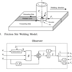
Welding direction Forwarding Side Welded zone Retreating Side x F y F z F Pin Shoulder

Fig. 3. Friction Stir Welding Model.

obs F g K G Γ c A ∫ ˆ Zɺ Zˆ θɺ θ u Saturation obs qɺ obs q Observer TJ M 4 ˆz 3 ˆz 2 ˆz T J D− − ˆ Z Z D − T obs J F

Fig. 4. Diagram of the observer

this process is to avoid those problems encountered in classical welding by melting the metals. It is for this reason that FSW process has been implemented, primarily in transportation industry where aluminum is used to reduce the weight of mechanical structures [2], [19]. Up to now, this process has been carried out by some specially developed machine-tools, which are expensive and have smaller workspace compared with robot manipulators.

III. OBSERVER DESIGN

FSW needs reliable force control and tracking performance under a significant axial force. This problem can be solved if the state of the links (q, ˙q) and external forces are known.

Unfortunately, only state and current of motor axes and axial force (Fz) are measured by our robot. Therefore, an observer

is proposed in this section to solve this problem.

Disturbance observer is a widely used technique in control for improving the performance of disturbance rejection [10]. The unknown input observer (UIO) method is one of the most well-known approach to estimate states [20]. The proposed observer is based on a non-linear observer introduced in [11], which reconstructs articular positions and velocities of links with the ones measured from motor axes. This observer is then modified in order to get also an estimation of efforts by adding more state variables function of forces. In this paper, the observer proposed in [12] has been improved to obtain a better performance in estimating external forces, the block diagram is presented Fig. 4, and it is then implemented into a KUKA robot for experimental validation.

If the state variables xi is defined as x1 = q =

[q1 q2 q3 q4 q5 q6]T, x2 = ˙q = [ ˙q1 q2˙ q3˙ q4˙ q5˙ q6˙ ]T,

x3= θ = [θ1θ2θ3θ4θ5θ6]T, x4= ˙θ = [ ˙θ1θ2˙ θ3˙ θ4˙ θ5˙ θ6˙ ]T,

then following state space model can be obtained:_         ˙ x1= x2 ˙ x2= ¨q = D(q)−1[Γ− H(q, ˙q) − Frobot( ˙q)− JT(q)F ] ˙ x3= x4 ˙ x4= ¨θ = Ia−1[Γm− N−TΓ− Fmotor( ˙θ)] (6)

Then, measured variables are now denoted as y, the following change of coordinates is considered:

             z1= [Ia−1N−TK]−1x4= K−1NTIax4 z2= x1= q z3= x2= ˙q z4=−D−1(z2)JT(z2)F y1= x3= θ y2= x4= ˙θ (7) Moreover, if u = Γ_ mthen:     ˙ z1= z2+ K−1NT[u− Fmotor(y2)]− Nvy1 ˙ z2= z3 ˙ z3= ¨q = z4+ ψ(z2, z3, y1) ˙ z4=−_dtd[D−1(z2)JT(z2)F ] (8)

where ψ is equal to:

ψ = D(z2)−1[K(Nvy1− z2)− H(z2, z3)− Frobot(z3)] (9)

If A and C are defined as following (I is the 6 order identity matrix and 0 is the 6× 6 zero matrix):

A =    0 I 0 0 0 0 I 0 0 0 0 I 0 0 0 0    and C = (I 0 0 0) (10) then: ˙ z = Az + g(z, y, u) + d(z, F, ˙F ) (11) with g =      K−1NT_{[u− F} motor(y2)]− Nvy1 0 ψ(z2, z3, y1) 0 (12) and d(z, F, ˙F ) = [0 0 0 −_dtd[D−1(z2)JT(z2)F ]]T.

This non-linear observer is an improved version of the one described in [12]. The measured input y1 and y2 are now θ

and ˙θ, z4 are here represent an additional acceleration which enables the additional acceleration ψ not to be a function of unknown disturbance external forces. Define now the following high gains matrix, with G a constant ≥ 1:

ΓG=    GI 0 0 0 0 G2_{I 0 0} 0 0 G3_{I 0} 0 0 0 G4_I    (13)

and matrix L such as (A− LC) has all its eigenvalues in the left half of the complex plane, then a new observer is proposed as follow: ˙ˆz = (A − ΓGLC)ˆz + g(¯z, y, u) + ΓGKy¯ 2 (14) where ¯K = LK−1NTIa and:      ¯ z2= y1−_∥yy1−ˆz2 1−ˆz2∥Nssat( ∥y1−ˆz2∥ Ns ) ¯ z3= zˆ3 ∥ˆz3∥Mssat( ∥ˆz3∥ Ms ) ¯ z4= zˆ4 ∥ˆz4∥Assat( ∥ˆz4∥ As ) (15)

with the saturation function:

sat(x) =

{

x if | x | ≤ 1

0 1 2 3 4 5 6 7 8 −0.02 −0.015 −0.01 −0.005 0 0.005 0.01 0.015 0.02 t [s] Angular velocity[rad/s]

axis1 axis2 axis3 axis4 axis5 axis6

Fig. 5. Estimate error of angular velocity.

and Ms, Ns, FM, Fd, JM, DM and As are known positive

physical constant bounds:                  ∥ x2∥< Ms ∥ x1− x3∥< Ns ∥ F ∥< FM ∥ ˙F ∥< Fd ∥ JT_(z 2)∥< JM ∥ D−1_(z 2)∥< DM As= DMJMFM (17)

Fig. 4 shows the diagram of the proposed observer where Ac=

A− ΓGLC. For only one axis, L = [L1L2L3L4]T and:

det[λI− (A − LC)] = λ4+ L1λ3+ L2λ2+ L3λ + L4 (18)

where λ is an eigenvalue of matrix A−LC. A possible choice for L is then: L1 = 4a, L2 = 6a2, L3 = 4a3 and L4 = a4.

In this case, matrix A− LC has four stable eigenvalues in

λ =−a, where a is a positive real fixing the dynamics of the

proposed observer.

The estimation error e = z − ˆz satisfies the following differential equation:

˙e = Ace + g(z, y, u)− g(¯z, y, u) + d(z, F, ˙F ) (19)

Because of the form of disturbance d(z, F, ˙F ) the following

stability theorem can be proven for the proposed observer:

Theorem 1: There exists a constant G0such that error e(t)

is bounded for any gain G > G0_.

The proof is similar to one described in [12], as ∥

d

dt[D−1(z2)JT(z2)F ]]T ∥ is bounded since ˙z2, F , F are˙

bounded (see equation (17)) and ∂D−1(z2)

∂z2 and

∂JT_(z

2)

∂z2 are

also bounded as they are only functions of sines and cosines.

IV. EXPERIMENTAL VALIDATION

A. Test 1: Validation of proposed observer during diving phase of FSW process

On the first step, the observer is validated only with measured data. FSW process can be divided into three phases: diving, welding and removing the tool. During experiment, the robot is programmed to press on a work-piece, then the tool will enter the material step by step with a force (Fz) equalling

0 1 2 3 4 5 6 7 8 9 −3500 −3000 −2500 −2000 −1500 −1000 −500 0 500 t [s] Force [N] Fxobs Fyobs Fzobs Fzmesured

Fig. 6. Comparison between measured force and estimated force.

Fig. 7. Block diagram for validation of force building in the case of a complex trajectory of robot KUKA KR500 MT-2.

1000 N, 2000 N and 3000 N, just like the diving phase of FSW process as shown in Fig. 1. Meanwhile, state of rotor (θ, ˙θ),

current of each motor (I) and the axial force Fzmeasured are

measured with the Scope and function monitor FTCtrlMonitor of the robot controller. After that, the state and current are used off line as input of the observer. The observer should reconstruct the state of link (qobs, ˙qobs) and the external forces

(Fxobs, Fyobs, Fzobs), as shown in Fig. 4. In this test, we have

chosen tuning parameters of the observer G = 1, a = 25 for the first three axes and a = 50 for the other axes. Moreover, the lateral forces in direction x and y are also estimated, which improves operation performance as it is these lateral forces that prevent the robot to weld a straight line during FSW process.

Fig. 5 shows the error of reconstructed angular speeds ( ˙qobs− ˙θl), as ˙θlis angular velocities after reduction gearbox.

As mentioned before, the tool is in contact with work-piece at the beginning. During this experiment, only the axes of motor can have a little movement while applying a force in

z direction, links of robot should rarely move. Fig. 6 presents

the estimated forces and the measured force Fzmeasured on

direction z of the tool frame, since the robot only has axial force sensor. The Fzobs matches well with the Fzmeasured,

and the observer has also reconstructed other forces Fxobsand Fyobs. Here, Fyobs might be caused by friction.

0 2 4 6 8 10 12 14 −2 −1.5 −1 −0.5 0 0.5 1 1.5 2 2.5 t [s] Angle [rad] θl1 θl2 θl3 θl4 θl5 θl6

Fig. 8. Robot KUKA KR500 MT-2 measured reference angle displacements.

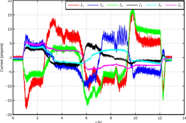
0 2 4 6 8 10 12 14 −20 −15 −10 −5 0 5 10 15 20 t [s] Current [ampere] I1 I2 I3 I4 I5 I6

Fig. 9. Robot KUKA KR500 MT-2 measured currents.

B. Test 2: Validation of observer in the case of a complete trajectory

On the second step, the robot is programmed to move along a large trajectory in its workspace.Fig. 8 and Fig. 9 present the measured angular displacements and currents on each motor axis. Then, the desired displacement, speed and acceleration measurements fed a simulation model of robot KUKA KR500 MT-2 disturbed by an external force, as shown in Fig. 7. From

t = 4s, an external force of Fz = 1000 N is added to the

robot system model. The reconstructed state of links (qobs,

˙

qobs) and external forces (Fxobs, Fyobs, Fzobs) are compared

with the measured state of motor axes (θl, ˙θl) and the added

forces to verify and validate the proposed observer. The results show a good performance in angular position, velocity and external force estimations as shown in Fig.11 with a precision of 10−7rad for positions and 10−5rad/s for velocities. Fig.

10 shows the torque due to the added external force on each axis, which can reach about 1400 Nm on axis 2. If we defined

χ = JT_F−(JT_{F )}

obs, then the relative mean square error can

be calculated by:

RM SE = χrms/(JTF )rms (20)

where χrms and (JTF )rms are the root mean square value

of χ and JTF respectively. The RM SE of axes 2, 3 and

5 are equal to: RM SE2 = 0.79%, RM SE3 = 0.83%,

RM SE5= 0.37%.

The identified inertia parameters have good precisions, but here, in order to analyse the sensitivity of the proposed observer, two simulations have been carried out with an additional error of ±10% of inertia parameters (see Fig.12

0 2 4 6 8 10 12 14 −1600 −1400 −1200 −1000 −800 −600 −400 −200 0 200 t [s] Torque [Nm] JTF1obs JTF2obs JT_F 3obs JTF4obs JTF5obs JTF6obs

Fig. 10. Estimated torques due to external force.

0 2 4 6 8 10 12 14 −2 −1 0 1 2x 10 −7 Position [rad]

Observer estimation errors

0 2 4 6 8 10 12 14 −10 −5 0 5x 10 −5 Velocitiy [rad/s] 0 2 4 6 8 10 12 14 −20 −10 0 10 20 30 t [s] Torque [Nm]

axis1 axis2 axis3 axis4 axis5 axis6

Fig. 11. Observer error of angular positions q− ˆq, velocities ˙q − ˆ˙q. and torques JTF− (JT_{F )}

obs

and Fig. 13). The estimations appear to be stable and quite accurate in spite of the error of inertia.

V. CONCLUSIONS

In this paper, a non-linear disturbance observer is proposed for flexible-joint industrial robots and a stability theorem has been introduced to prove the boundedness of observer estimation errors. A flexible model of the concerned KUKA robot has been developed, with precise identification param-eters. A series of experimental validation tests demonstrates that the proposed observer is fast enough to estimate the system state with required accuracy and sensitivity, and better performance than the one proposed in [12]. Even under noises of measurement, this observer still provides satisfactory results in both state and external force estimations.

More precisely, in FSW diving phase, the estimated axial force matches well with the measured force. This method can also be applied to other robots and processes. For instance, in our laboratory, numerous experiments have been implemented to identify all the necessary parameters of KUKA KR500 MT-2. With more precise robot identification, the performance of observer can also be improved. Using both state of the rotor axes and the estimated state of robot links in the control of flexible robots can lead to more stable and robust feedback control as shown in [12], [17]. Moreover, the reconstructed external forces can reduce the error on the work-piece. Next step consists now to implement some experiments on-line with industrial robots, and use the estimated lateral force to suppress lateral deviation observed in FSW process.

0 5 10 15 −2 −1 0 1 2x 10 −6 Axis 2

errqobs[rad]

observer In+ 10% In − 10% 0 5 10 15 −4 −2 0 2 4x 10 −6 Axis 3 0 5 10 15 −5 0 5 10x 10 −7 t [s] Axis 5 0 5 10 15 −4 −2 0 2 4 6x 10

−4 err˙qobs[rad/s]

0 5 10 15 −1 −0.5 0 0.5 1x 10 −3 0 5 10 15 −4 −2 0 2 4x 10 −4 t [s]

Fig. 12. Comparison of estimation error of ˆq and ˆ˙q with±10% error of

Inertia parameters. 0 2 4 6 8 10 12 14 −2000 −1000 0 1000 Axis 2

Comparison JTFwith observer estimations (Nm)

JTF I n I n+ 10% I n− 10% 0 2 4 6 8 10 12 14 −1500 −1000 −500 0 500 Axis 3 0 2 4 6 8 10 12 14 −400 −200 0 200 t [s] Axis 5

Fig. 13. Comparison of JT_{F estimation error with±10% error of Inertia}

parameters.

APPENDIX ACKNOWLEDGMENT

This study is a part of the project ANR-2010-SEGI-003-01-COROUSSO that is sponsored by the French National Agency of Research as a part of the program ANR-ARPEGE.

REFERENCES

[1] S. Zimmer, L. Langlois, J. Laye, and R. Bigot, “Experimental inves-tigation of the influence of the fsw plunge processing parameters on the maximum generated force and torque,” Int. Journal of Advanced

Manufacturing Technology, vol. 47, no. 1-4, pp. 201–215, 2010.

[2] R. S. Mishra and Z. Y. Ma, “Friction stir welding and processing,”

Materials Science and Engineering,Reports, vol. 50, pp. 1–78, 2005.

[3] G. Besanc¸on, Nonlinear Observers and Applications, 1st ed., G. Besanc¸on, Ed. Berlin Heidelberg: Springer, 2007.

TABLE II. NUMERICAL VALUES OF ROBOTKUKA KR500 MT-2

N (i, j) Link length (m) Rigidity (N m/rad)

N11 469.375 L1x 1.045 K1 6.61 106 N22 469.375 L1z 0.500 K2 7.16 106 N33 −504.770 L2 1.300 K3 3.08 106 N44 −260.619 L34 1.025 K4 0.56 106 N55 −251.977 D4 −0.055 K5 0.66 106 N66 164.570 L5 0.290 K6 0.47 106 N54 −1.0964 Ltz 0.350 N64 −1.5836 Lty 0 N65 1.5311

[4] S. E. Talole, J. P. Kolhe, and S. B. Phadke, “Extended-state-observer-based control of flexible-joint system with experimental validation,”

IEEE Transactions on Industrial Electronics, vol. 57, no. 4, pp. 1411–

1419, 2010.

[5] A. De Luca, D. Schr¨oder, and M. Th¨ummel, “An acceleration-based state observer for robot manipulators with elastic joints.” in IEEE

International Conference on Robotics and Automation, Roma, Italy,

April 2007, pp. 3817–3823.

[6] R. Henriksson, M. Norrl¨of, S. Moberg, E. Wernholt, and T. B. Sch¨on, “Experimental comparison of observers for tool position estimation of industrial robots,” in Proceedings of the IEEE Conference on Decision

and Control, 2009, pp. 8065–8070.

[7] C. Kravaris, V. Sotiropoulos, C. Georgiou, N. Kazantzis, M. Q. Xiao, and A. J. Krener, “Nonlinear observer design for state and disturbance estimation,” Systems Control Letters, vol. 56, no. 11-12, pp. 730–735, 2007.

[8] T. A. Davis, Y. C. Shin, and B. Yao, “Observer-based adaptive robust control of friction stir welding axial force,” IEEE/ASME Transactions

on Mechatronics, vol. 16, no. 6, pp. 1032–1039, 2011.

[9] B. Yao and L. Xu, “Observer-based adaptive robust control of a class of nonlinear systems with dynamic uncertainties,” International Journal

of Robust and Nonlinear Control, vol. 11, no. 4, pp. 335–356, 2001.

[10] S. K. Park and S. H. Lee, “Disturbance observer based robust control for industrial robots with flexible joints,” in International Conference

on Control, Automation and Systems 2007. Seoul, Korea: ICCAS ’07,

December 2007, pp. 584 – 589.

[11] M. Jankovic, “Observer based control for elastic joint robots,” IEEE

Trans. on Robotics and Automation, vol. 11, no. 4, pp. 618–623, 1995.

[12] J. Qin, F. L´eonard, and G. Abba, “Non-linear observer-based control of flexible-joint manipulators used in machine processing.” in Proceedings

of The ASME 2012 11th Biennial Conference on Engineering Systems Design and Analysis, no. 82048, Nantes, France, July 2012.

[13] W. Khalil and E. Dombre, Modeling, Identification and Control of

Robots, K. P. S. Paper, Ed. Oxford: Elsevier Ltd, 2004.

[14] SYMORO+ Symbolic Modeling of Robots, User’s Guide.

[15] W. Khalil and D. Creusot, “Symoro+: A system for the symbolic modelling of robots,” Robotica, vol. 15, pp. 153–161, 1997.

[16] M. W. Spong, “Modeling and control of elastic joint robots,” Journal

of Dynamic Systems, Measurement, and Control, vol. 109, no. 4, pp.

310–318, 1987.

[17] M. W. Spong, S. Hutchinson, and M. Vidyasagar, Robot Modeling and

Control, M. Spong, S. Hutchinson, and M. Vidyasagar, Eds. Berlin

Heidelberg: John Wiley and Sons, Inc., 2005.

[18] R. Nandan, T. DebRoy, and H. Bhadeshia, “Recent advances in friction-stir welding - process, weldment structure and properties,” Progress in

Materials Science, vol. 53, no. 6, pp. 980–1023, 2008.

[19] X. Zhao, P. Kalya, R. G. Landers, and K. Krishnamurthy, “Empirical dynamic modeling of friction stir welding processes,” Journal of

Man-ufacturing Science and Engineering, Transactions of the ASME, vol.

131, no. 2, pp. 1–9, 2009.

[20] X. Yue, D. Vilathgamuwa, and K.-J. Tseng, “Robust adaptive control of a three-axis motion simulator with state observers,” IEEE/ASME