Quantitative thermal analysis of heat transfer in liquid–liquid biphasic millifluidic droplet flows

Science Arts & Métiers (SAM)

is an open access repository that collects the work of Arts et Métiers Institute of

Technology researchers and makes it freely available over the web where possible.

This is an author-deposited version published in: https://sam.ensam.eu Handle ID: .http://hdl.handle.net/10985/9354

To cite this version :

Marta ROMANO, Christophe PRADERE, Jean TOUTAIN, Cindy HANY, Jean-Christophe BATSALE - Quantitative thermal analysis of heat transfer in liquid–liquid biphasic millifluidic droplet flows - Quantitative InfraRed Thermography - Vol. 11, n°2, p.134-160 - 2014

Any correspondence concerning this service should be sent to the repository Administrator : archiveouverte@ensam.eu

Quantitative thermal analysis of heat transfer in liquid–liquid

biphasic milli

fluidic droplet flows

Marta Romanoa, Christophe Pradereb*, Jean Toutainb, Cindy Hanya and Jean Christophe Batsaleb

a

LOF, Université Bordeaux 1, UMR CNRS-Rhodia-UB1 5258, Pessac Cedex, France; bI2M, TREFLE Département, UMR CNRS 5295 – site ENSAM Esplanade des Arts et Métiers, Talence

Cedex, France

(Received 29 April 2013; accepted 6 June 2014)

In this paper, infrared thermography is used to propose a simple quantitative approach toward understanding the thermal behaviour of a liquid–liquid biphasic millifluidic droplet flow under isoperibolic conditions. It is shown that due to the isoperibolic boundary condition, the thermal behaviour at the established periodic state can be managed according to different orders, i.e. either a continuous or fluctuating contribution. A complete analytical solution is proposed for the complex problem model, then a simplified model is proposed. Finally, a simple homogeneous equivalent thin body model approximation with a characteristic coefficient function of a biphasic flow mixing law is sufficient for describing the thermal behaviour of the media under isoperibolic conditions. From this theoretical validation, the experimental results concerning the behaviour of a biphasic oil and droplet flow are presented. An analytical representation law is proposed to quantitatively estimate and predict the thermal behaviour of the flow. Moreover, it is demonstrated that with this new method, the thermophysical properties of the phase can be estimated with a deviation less than 5% from that reported by the suppliers.

Keywords: biphasic flow; infrared thermography; millifluidics; thermophysical property estimation; heat transfer

1. Introduction

Infrared thermography is a versatile technology that can be applied under a very wide range of domains and scales, ranging from macroscopic applications, such as building and agriculture diagnostics,[1,2] to the observation of miniaturised systems, such as elec- tronic device characterisation or biological and chemical systems.[3,4] More precisely, for quantitative studies, this technology offers the possibility to measure important exper- imental parameters, such as the convective heat transfer,[5] as well as to monitor the tem- perature distribution,[6] which can be one of the most important parameters in some experimental studies. In this study, this versatile technology has been combined with miniaturised fluidic systems that have proven to be novel and important tools for online chemical analysis and process intensification. In such systems, the transport phenomena are enhanced, allowing the study of chemical reactions or phase transitions under a wide range of configurations.[7–9] Some micro-fluidic systems have already been combined with infrared thermography to study different phenomena, such as the thermal analysis

of nanofluids,[10] the temperature profiles in micro-reactors,[11] the monitoring of exo- thermic reaction stability [12] and the measurement of the temperature of small amounts of liquid in micro-fluidic chips.[13] Moreover, in the field of micro-fluidics, many react- ing chemical flows are carried out for thermochemical analysis. The first theoretical and numerical studies of chemical reactions [14,15] were performed in straight channels within continuous flow systems. In this configuration, at the inlet of the channel, a simple interdiffusional mixing zone is established; the length of this zone is mainly handled by the inner diameter of the channel, as well as by the diffusion coefficient. Some tech- niques have also been developed to quantify the heat released by a chemical reaction. Wang et al. [16] measured the temperature in miniaturised systems using detached sensors to estimate the reaction enthalpy. Other studies have shown the possibility to carry out a well-adapted calorimetry analysis of the experimental micro-fluidics condi- tions.[17,18] Some infrared thermography studies have been carried out under coflow conditions, where the diffusion limitation due to species mixing is thoroughly demon- strated.[19,20] Then, to overcome the problem of diffusion limitations and to intensify reactant mixing, the flow analyses were performed using droplets. Based on this new hydrodynamic configuration, many studies were dedicated to the characterisation of physical behaviour.[21–23] Today, a wide range of physical and chemical phenomena are studied based on the droplet configuration. The main advantage of such biphasic flows (i.e. droplets) is a consideration of the droplet as an independent reactor. In this case, homogenous mixing can be achieved faster by implementing chaotic advection,[24] as well as by establishing hydrodynamic recirculation inside the droplet.[25] Some numerical studies concerning the thermal effects of heat transport in a droplet-laden flow [26] have also been studied. Moreover, many experimental and theoretical works concerning the thermal effects and thermal characterisation of segmented liquid gas flows have been presented.[27–29] Most of these studies concern the cooling systems of minia- turised electronic devices, which are used to improve micro-heat exchangers.

Nevertheless, neither experimental nor analytical thermal characterisations of liquid–liquid droplet flows in millifluidic systems have been studied to date. Here, we paid particular interest to developing an understanding of the heat exchanges that occur in isoperibolic biphasic flows under various imposed temperatures, total flow rates and ratios. In this first study, no heat source is added to the droplets as a result of chemical reaction or phase change. Nevertheless, it is relevant in such configurations to develop a better understanding of the thermal heat transfer mechanism before studying any chemical reactions, phase change transitions, species mixing or wetting processes, which are generally strongly influenced by the effects of temperature.

In this paper, it will be shown that due to the very good hydrodynamics stability of the flow, direct thermal analysis in the droplet space becomes possible (Lagrangian). Based on this assumption, and starting from a complete analytical solution, it will be demonstrated that the effects of thermal diffusion inside biphasic media under flow can be well approximated by a convective two-temperature (2T) thin body model. Then, it will be shown that this representative model can be decomposed into a sum of continu- ous and fluctuating contributions. Further, due to the very weak influence of the fluctu- ating contribution (less than 2%), it will be shown that from a thermal point of view, the continuous temperature contribution is a very good approximation of the global thermal behaviour of such biphasic systems under flow. From this model, and using an inverse processing method applied to several experimentations, this approach is then validated. This analysis can then lead to an estimation of the characteristic coefficient (the inverse of time or length), which is due to convective effects. The relationship

between the total flow and the segmented flow rate ratio is discussed later. Moreover, from these experimental measurements, an analytic thermal law is proposed. Finally, it is interesting to note that this expression results from a biphasic mixing law that allows for the estimation of thermal parameters, such as the characteristic coefficient and ther- mal properties, like the specific heat of the fluids. Based on this calibration study, it is shown that this non-intrusive, online technique is well adapted for monitoring and quantifying the thermal behaviour of miniaturised biphasic flows.

2. Experimental consideration

2.1. Description of the experimental set-up

The millifluidic reactor shown in Figure 1(A) was designed using a bulk piece of brass for thermal control, whereas the flow set-up was realised inside of small-sized commercial perfluoroalkoxy (PFA) tubing and junctions (from Jasco). The bulk brass (Figure 1(A)) is thermally regulated (with a PID system) using a Peltier module with a temperature range from −5 to 70 °C for the accurate cooling and heating of the tubes inserted into the grooves of the bulk metal piece. Because PFA tubing is a good thermal insulator (ktube = 0.10 W m−1 K−1) and bulk brass is a good thermal conductor (kp = 380 W m−1 K−1), the boundary condition of the external diameter of the tubing is

assumed to work at the imposed temperature (i.e. isoperibolic). A heat sink paste was added between the tube and the brass plate. Consequently, the temperature inside the chemical reactor results from the heat transfer coefficient between the imposed tempera- ture of the bulk brass and the inner diameter of the tube. Inside the tubing, the biphasic flow is delivered by a high-precision syringe pump (NEMESYS from Cetoni), where the oil (also called continuous phase) and droplets are generated by the injection of both fluids at different ratios. This allows for control of the hydrodynamic parameters, which include the total flow rate (i.e. the droplet velocity), the droplet size and the ratio between the oil and droplets. At the inlet of the tube schematic (Figure 1(B)), droplet generation is carried out using smaller tubes to deliver the reactants. The dimensions of the PFA tubing are 3.17 mm for the outer diameter and 1.6 mm for the inner diameter. The tubes used to supply the reactants have an outer diameter of 500 µm and an inner diameter of 350 µm.

Figure 1. (A) Schematic of the experimental set-up for bulk brass and isoperibolic chip, (B) schematic of the injection system of the droplets and (C) assembly of the experimental set.

An infrared CEDIP camera (model JADE MWIR J550) is used for the temperature field measurements (Figure 1(C)). The IR sensor is a 240 × 320 pixel InSb focal plane array optimised for wavelengths ranging from 2 to 5.2 µm and a pitch of 30 µm. The IR objective lens is a 25 mm MWIR. With this objective, the spatial resolution of the temperature measured by each pixel of the sensor is approximately 250 µm in the object plane. A visible camera is also used to measure the droplet flow to estimate the velocity. This camera has a CCD sensor (Sony ICX445) with a size of 1/3, an optimum wavelength ranging from 400 to 700 nm and a pitch of 4 µm. Finally, a 16 mm visible objective (1/3 sensor size) is used, allowing for a spatial resolution of 60 µm.

2.2. Spectroscopy study of transparency and emissivity of the tubing

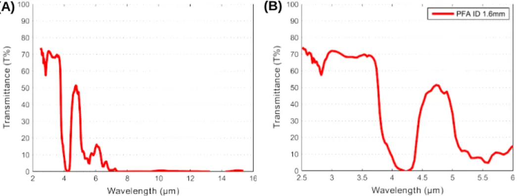
The degree of transparency of the PFA tubing at the IR wavelength used in the study was characterised using infrared spectroscopy. The transmittance spectra of the tube in the wavelength range from 2.5 to 15 µm are illustrated in Figure 2(A). Figure 2(B) shows only the results in the IR range of the camera. It should be noted that the selected tube is semi-transparent at the camera wavelength, so it is important to analyse the emissivity behaviour of the biphasic media.

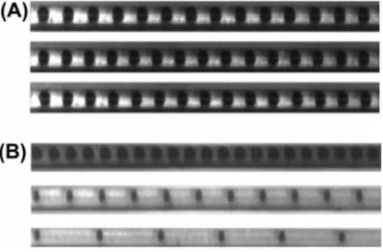
In Figure 3, the principle of the experiment is sketched. A PFA tube was half filled with oil and half with water (coloured blue); additionally, a second tube was placed in the adjacent groove and filled with air, as depicted in the visible image presented in Figure 3(A). The initial temperature of the brass chip at t ¼ 0 s was equal to the room temperature (20 °C). Then, the brass chip temperature was increased to Tp = 30 °C. In this transient study, three stationary phases (air, oil and water) were analysed. After image analysis, the temperature profiles of the phases as functions of time were extracted to identify the emissivity behaviour when a thermal constraint is applied.

Figure 4 shows these profiles as functions of time. The observed thermal responses are expressed in terms of digital levels (DL). In this figure, due to the spatial thermal gradient, the intensity levels of the brass chip, the air tube and the biphasic media at

t ¼ 0 s are not at the same initial level, even if the initial temperature is the same (see

also Figure 3(B)). Then, when the temperature is increased to Tp = 30 °C at t ;:: 3 s, the transient response of each medium is different and linked to the respective thermophys- ical properties of the medium, as shown in Figure 3(C). Finally, when steady state is

(A) (B)

Figure 2. (A) Infrared spectra of the selected tubes. (B) Magnified presentation of the wavelength range of the infrared camera.

T emp er at u re d if fer en ce , ( DL ) DIFFERENCE OIL − WATER (B) 10 20 30 40 50 Time (s) 60 T emp er at u re v a ri a ti o n , ⊗ T ( DL )

Figure 3. (A) Visible image of the experimental PFA tubing, half filled with oil and half with water (coloured blue). A second piece of tube was filled with air. (B) An IR image of the experiment at t ¼ 0 s. (C) An IR image of the experiment at t ¼ 10 s. (D) An IR image of the experiment at t ¼ 60 s. (A) 1400 1200 1000 AIR WATER OIL 800 80 60 600 40 400 20 200 0 0 0 50 100 150 200 250 Time (s)

Figure 4. (A) Temperature profiles variation according to the initial values (DT ) of the three sta- tionary media (air, oil and water) when a thermal constraint is applied from Tp = 20–30 °C. (B)

Temperature difference between the oil and the water. Note that the initial emissivity was subtracted.

reached at t ¼ 60 s, the three phases have reached the same imposed temperature, i.e. the temperature of the brass is Tp (see also Figure 3(D)). At this time, the biphasic

emissivity values (see Figure 4(B)). In contrast, it can be observed that for the same temperature, the tube full of air appears to be cooler than the biphasic media tubing. Thus, it can be concluded that the water and oil phases are more opaque than air and that both fluids have nearly the same values of emissivity.

It is important to note that for further experimental work, because the tubing is semi-transparent, the measured temperature integrates a portion of the tubing volume; however, the transient thermal response is representative of the thermal behaviour of the biphasic media, which will be assumed to be an opaque body. Additionally, the IR camera studies were carried out in the range of linearity according to the temperature (experimental calibration not shown here).

3. Description of the proposed method

3.1. Velocity stability validation using visible wavelength data

It is important to highlight the benefits of such biphasic systems under flow. First, as shown in Figure 5, when using the syringe pump, the flow rate ratio (R) between the continuous phase (oil, QO) and the droplets (water, QD) is easily mastered. For example

(Figure 5(B)), for a given total flow (QT ), it can be observed that the length and the

shape of the droplets are significantly modified by changing the R ratio. From a thermal point of view, this will significantly affect the thermal behaviour (i.e. the heat transfer) between the droplet and the oil and, in particular, the heat exchange surface between the fluid and the wall. Moreover, in Figure 5(A), for an imposed ratio R, the length and the shape are independent of the total flow rate variation. From the thermal and chemi- cal points of view, increasing the total flow only affects the residence time and the flow velocity by increasing the temporal resolution. It is important to note that the droplets are generated before entry into the isoperibolic chip to avoid droplet break-off due to the fluid stream (the continuous phase).

From the visible images, the length of each phase (the droplet and the oil) is calcu- lated using an edge detection image processing algorithm. The velocities at different total flow rates and ratios were estimated by the displacement of the edges. In Figure 6, the oil length increases with increasing flow rate ratio, while the droplet length decreases to a constant value. Figure 7 shows that the mean velocity U- remains almost

Figure 5. (A) Visible image of the droplet flows for three different total flow rates (QT ) with a

constant ratio R =2 (QO /QD = 2), from top to bottom QT = 10, 20 and 30 mL h-1. (B) Visible

image of the droplet flows with a constant total flow rate (QT = 20 mL h−1), and various oil–water

Figure 6. The length ratio alpha (a = LD=LO) as function of the flow rate ratio R measured from

the visible images at QT = 20 mL h−1. At the top right corner of the graph, the raw lengths for

the droplet LD and for the oil LO as functions of the flow rate ratio can be observed. The flow

rate ratio (R) ranges from 1 to 15. For R = 1, the same flow rate was imposed on the oil and droplets, whereas R = 15 means that the imposed oil flow rate was 15 times higher than that of the droplets. The reported error bars correspond to the dispersion results obtained from repeated experiments.

constant when the flow rate ratio R is varied. The calculated error bars correspond to the dispersion results obtained in repeated experiments.

From these flow pattern measurements, it is clearly demonstrated that the hydrody- namics in such systems are perfectly controlled, ensuring good stability and reproduc- ibility of the droplet sizes and velocities. According to these observations, it is proposed that the work be carried out within the space of the droplet (the local coordi- nate system used to develop the thermal model). This can be accomplished when the droplet flow velocity has been previously calculated to track the biphasic plug along the chip.

3.2. IR validation of the thermal periodic established state

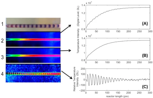
In Figure 8, different temperature fields are reported to demonstrate that the spatial evo- lution of the temperature is periodic. In this validation, the initial values of the tempera- tures of both the water and oil phases are equal to room temperature (20 °C) and the bulk brass, imposed at 30 °C, but are expressed on DL units. The thermal phenomena can be managed according to different orders. The observation of the IR raw tempera- ture profile in Figure 8(A) demonstrates that the signal is composed of a continuous

Figure 7. Measured mean velocity U- (cm s−1) of the biphasic flow as a function of the flow rate ratio R, at different total flow rates QT .

contribution (of order 1, see Figure 8(B)) and a fluctuating contribution (of order 2, see Figure 8(C)) according to the following expression:

T ðz; tiÞ ¼ T ðzÞ þ T~ðz; tiÞ (1)

The fluctuating component highlights the presence of the biphasic flow, as shown in Figure 8(C), but represents less than 2% of the average signal of the continuous flow (T ðzÞ, Figure 8(B)). The continuous component (CC) resulting from the average value over N periods of each pixel of the channel is a function of the volume ratio of each phase. This is similar to achieving an overall space average in the local coordinate of the droplet–oil space.

The different orders of the thermal behaviour of the biphasic flow are highlighted in Figure 8. The raw profiles for a given ratio R at different positions of the channel are shown in Figure 9(A). The profiles have periodic fluctuations given by the oil and droplet flows. To enhance the biphasic thermal behaviour, the average value of the established state can be subtracted (Figure 9(B)). At the end of the channel, where the imposed temperature is reached, the phases of the droplets and the oil cannot be distin- guished (Figure 9(A) and (B), the pixel 280 is plotted as - · - · -).

Finally, from this validation, we can assume from a thermal point of view that a model of two diffusive media in Lagrangian space is sufficient to represent the thermal behaviour of such a system. From an experimental point of view, the periodicity of the

(A)

(B)

(C)

Figure 8. Schematic of the thermal phenomena at different orders: (1) Visible image of the droplet flow at time t. (2) Infrared images of the temperature field measured at time t. (3) Averaged field over N periods. (4) Field of the fluctuating component. Right side: (A) Tempera- ture profile along the channel at time t (T ðz; ti)) from image 2, (B) temperature profile along the

channel, where the temperature field is averaged over N periods T ðzÞ, (C) fluctuating profile along the channel T~ðz; tiÞ, obtained when signal B is subtracted from the field on signal A.

Figure 9. (A) Raw temperature profiles at several positions as functions of the acquisition time (frames). (B) Relative temperature profiles when the mean average at the same pixel is subtracted at several positions as a function of the acquisition time (frames).

flow could be considered as an advantage with respect to signal averaging to significantly increase the signal-to-noise ratio.

4. Thermal modelling

4.1. Analytical description of the isoperibolic condition

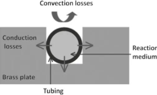
Figure 10 illustrates a cross-sectional representation of the isoperibolic system, from which it can be noted that 3=4 of the tube is in contact with the brass plate, which induces the conductive heat transfer.

The 1=4 of the tube (v) that is in contact with the ambient may have a heat exchange coefficient of approximately h = 10 W m−2 K−1. Further, if we consider the thickness etube ¼ 800 μm and ktube = 0.10 W m−1 K−1, a steady-state energy balance with

a heat source (/, W) inside the tubing is proposed according to the following expression:

/ ¼ hSaðTtube - TaÞ þ hpSpðTtube - TpÞ (2)

Here, h (W m−2 K−1) is the coefficient of heat loss as a result of convection with the surrounding atmosphere through 1=4 of the tubing perimeter, whereas hp

(W m−2 K−1) is the thermal conductance due to heat transfer by conduction through the thickness of the tubing (i.e. the isoperibolic condition) in the 3=4 of the tubing perime- ter, and S (m2_{) is the heat exchange surface. From this con}figuration, Equation (2) can

be rewritten as follows:

1 ktube 3

/ ¼ h

4 pdLðTtube - TaÞ þ etube4 pdLðTtube - TpÞ; (3) where Ta (K) is the temperature of the surrounding, Tp (K) is the temperature of the

brass chip and d (m) is the diameter. The calculation of the ratio Rhl between the ther-

mal resistances of conduction and convection are calculated as follows: Rhl ¼ vpdLhetube ð1 - vÞpdLktube with v ¼ 0:25 Rhl ¼ 1 hetube 3 ktube 1 10-1 (4) ¼ 3

The estimated value Rhl = 3.33 × 10-2 is smaller than unity; this fact allows us to

neglect the convective heat losses compared to the conduction losses (i.e. the isoperibolic condition). In further development, the system is considered to be completely isoperibolic with a value of 1 and not the alternative (1 − v).

i 4.2. Statement of the problem

When a biphasic flow is performed in a millimetric isoperibolic device, the hydrody- namic assumptions concerning the velocity approximation and periodic established state can be considered. Thus, the complete thermal problem can be taken as a 2-D axisym- metric two-layer periodic system (r, z, t), as represented in Figure 11.

Because the goal of our study is to perform data processing to quantify the thermal behaviour of the system, the idea is to develop a simplified thermal model that allows for a good representation of the complete system. First, due to the very large ratio between the lengths of the biphasic plug versus that of the diameter of the tubing, it is assumed that the temperature along the radial direction (r) is quasi-constant. Then, the thermal problem can be approximated only in the z-direction. Consequently, the mea- sured temperature over the channel is averaged in the r-direction to obtain the T ðz; ti)

function of the space, z, and time, t.

4.3. Complete model of the biphasic plugs in Lagrangian space

The complete model is schematised in Figure 11. The model consists of a two-media system that is believed to be in perfect contact for a half plug of water and a half plug of oil. We assume that convective exchanges exist between each phase and the bulk (described by the same heat exchange coefficient hp in W m−2 K−1), and that thermal

diffusion occurs inside and between each medium. With this representation, the left and right boundaries of the system are adiabatic (for symmetry reasons). Thus, the general heat transfer equation of each medium can be expressed as follows:

@2_T iðz; tÞ 1 @ Ti ð z ; t Þ where @z2 þ Uðz; tÞ - HiðTiðz; tÞ - TpÞ ¼ _a (5) @t (A) (B)

Figure 11. (A) Visible and thermal images of the local coordinate system (Lagrangian) of one droplet–oil period. (B) Schematic of the heat exchanged between the droplet (water), the continuous phase (oil) and the wall (brass plate) through the tubing.

i d p k i D - D O - k 2 /DðtÞ Uðz ¼ 0 to LD; tÞ ¼ D and Uðz ¼ LD to LT ; tÞ ¼ 0; (6)

where T (K) is the temperature along the z-direction, H (m-2) is the effective character- istic coefficient between each medium and the bulk, and a (m2 s−1) is the thermal diffu- sivity of both fluids, where the index i can denote either the droplet (D) or the oil (O) and /_Dðz; tÞ represents the heat source (in W) in the droplet (in this study, the heat source is limited to the chemical reaction, if any, occurs).

H 4hp (7)

i ¼ kid

The value of hp (W m−2 K−1) is defined by the convective heat exchange coefficient,

the thermal conductivity k (W m−1 K−1) and the inner diameter d (m). The calculations are presented directly in Laplace space using the following transformation:

Hiðz; pÞ ¼

Z t¼þ1 t¼0

Tiðz; tÞe-pt dt (8)

According to Equation (8), the integrated temperature in Laplace space for either the droplet (HD) or the oil (HO) is represented. As well as the integrated source in

Laplace space.

Z t¼þ1

GðpÞ ¼ t¼0

GðtÞe-pt dt with G ¼ U or G ¼ /_D (9)

Due to the isoperibolic condition, the temperature of the wall (TP ) is held constant.

Equation (5) is rewritten in the Laplace domain using Equations (8) and (9) as follows:

d2H iðz; pÞ p \ Ti ð0Þ 4 h p T p dz2 - Hi Hi þ _a ¼ - _a i - k d p - GðpÞ (10)

Equation (10) is rewritten for each phase in the Laplace domain. First, the equation for the droplet is presented as follows:

d2H Dðz; pÞ p \ TD ð 0 Þ 4 h p Tp dz2 - HDðz; pÞ HD þ _a ¼ - _a D k d p - GðpÞ for z ¼ O to LD (11)

Then, the equation for the oil plug is expressed as:

d2HOðz; pÞ p \ T O ð 0 Þ 4 h p T p with: dz2 - HOðz; pÞ HO þ _a ¼ - _a O for z ¼ LD to LT (12) O 4hp b p and b2 4hp p (13) D ¼ _k Dd þ aD O ¼ kOd þ aO

b b D ð Þ O ð Þ 0 B Dð D Þ ¼ Oð D Þ ¼ D a - D O - e k ¼ TD ð0Þ 4 h p Tp TO ð 0 Þ 4 h p Tp SDðpÞ ¼ - D _{k d p} - UðpÞ; SOðpÞ ¼ - a (14) kOd p

The solution for the non-homogeneous ordinary differential equations (11) and (12) is given by: HDðz; pÞ ¼ Ae-bD z þ BebD z - S D ð p Þ 2 D ; HOðz; pÞ ¼ A0e-bO z þ B0ebO z - S O ð p Þ 2 O (15) Thus, the boundary conditions schematised in Figure 11(A) are expressed in Equations (16)–(19):

d H z; p

dz ¼ 0 at z ¼ 0 and

d H z ; p

dz ¼ 0 at z ¼ LT (16)

Rewriting the general solution for the droplet and oil, the following equations are obtained by applying the boundary conditions, expressed as follows:

HDðz; pÞ ¼ HD0 ðpÞ þ A e -bD z þ ebD z) for z ¼ O to LD (17) HOðz; pÞ ¼ HO ðpÞ þ ( e-bO z bO ðz-2LT Þ \ þ for z ¼ LD to LT (18)

The continuity (drop–oil interface) at LD of the temperature and the heat flux is

taken as: -kD d H D ð z ; p Þ dz ¼ -kO d HO ð z ; p Þ and H L ; p H L ; p at z L (19) dz

Applying the boundary conditions to develop a solution of the temperature profile for each phase, the general solution for the droplet temperature profile from z ¼ 0 to

LD is obtained:

HDðz; pÞ ¼ HD0 ðpÞ þ H0e

-bD ðLD -zÞ

ð1 þ FEÞð1 þ e-2b_D LD _Þ ð1 þ e

-2bD z _{Þ (20)}

Applying the boundary conditions from z ¼ LD to LT (where LT ¼ LD þ LO), the

general solution for the oil temperature profile is:

where HOðz; pÞ ¼ HO0 ðpÞ þ H0FEe -bO ðz-LD Þ ð1 þ FEÞð1 þ e-2bO LO _Þ ð1 þ e -2bO ðLT -zÞ_{Þ; (21)} kDbD ð1 - e-2bD LD Þð1 þ e2bO LO Þ F ObO and E ¼ ð1 þ e-2bD LD _{Þð1 - e}2bO LO _Þ (22)

p

Additionally, the offset terms are calculated according to the following expressions:

HD aD Tp / ðp Þ H O a O T p TD0 þ p þ qD CpD TO0 þ _p HD0 ðpÞ ¼ _{p þ H} DaD ; HO0 ðpÞ ¼ þ HOaO (23) H0ðpÞ ¼ HO0 ðpÞ - HD0 ðpÞ (24)

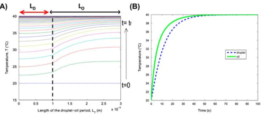
From the solutions expressed in Equations (20) and (21), a numerical inverse Laplace transform in the time domain (t) is performed using the Den Iseger algo- rithm.[30] From the analytical solutions, the temperature profiles in Figure 12 are gen- erated; in this case, no heat source was added (U = 0). The respective heat exchange coefficients h were estimated to be in the order of magnitude of hp = 150 W m−2 K−1.

More precisely, Figure 12(A) shows the analytical solution of the temperature pro- file of the droplet–oil length (LT ¼ LD þ LO); the solution is represented as function of

the space, corresponding to the period length. Due to heat transfer by convective diffu- sion, each of the phases evolved differently according to the respective thermophysical properties. Figure 12(B) represents the temperature of each phase shown in Figure 12(A) as a function of time. It can be observed that at the initial time t ¼ 0 s, both phases have the same initial temperature, whereas at the long timescale of t ¼ 50 s, both fluids tend to approach the temperature of the plate Tp = 40 °C. This complete thermal model takes into account the diffusive heat exchanges inside each medium, as well as at the interface in terms of the diffusion between the droplet–oil and, finally, the convective heat exchanges between the liquid and the isoperibolic bulk. The assumed hypothesis for simplifying the thermal model is shown to be well selected. It is demonstrated that a 1 − Dt biphasic analytical model is sufficient for representing the heat transfer in such a complex system.

Figure 12. (A) Calculated temperature profiles along the z-axis as functions of time for TD0 = 20 °C and TO0 = 20 °C, where the imposed wall temperature is Tp = 40 °C, for a given ratio

of R = 2 corresponding to the droplet oil length LD =1 mm LO = 2 mm. (B) The average

temperature profiles of (A) over the z-direction of each phase are represented as functions of time.

LD

q q q

L L

q

q

4.4. Simplified 2T thin body model in Lagrangian space: the fluctuating component

The main idea here is to propose a simplified model with simple convective exchange using an average temperature profile for each phase to model the diffusion in Lagrang- ian. The Biot number is calculated as Bi ¼ hL=k; for flow rate ratios at R ;:: 4, the Bi values are 0.34. In this case, Bi is lower than 1, implying that the temperatures of both phases are highly spatially homogenous.

By applying this thin body hypothesis, the convective–diffusive equations (11) and (12) can be rewritten as a simple 2T thin body model:

dTD ðt Þ

dt ¼ -HDP ðTDðtÞ - TP Þ - HDOðTDðtÞ - TOðtÞÞ þ UðtÞ (25)

dTO ðt Þ

dt ¼ -HOP ðTOðtÞ - TPÞ - HODðTOðtÞ - TDðtÞÞ (26)

The temperature profiles of the droplet (TD) and of the oil (TO) result from the

average over the space, according to Equation (27). R LD TDðz; tÞdz R LTTOðz; tÞdz TDðtÞ ¼ 0 D ; TOðtÞ ¼ O (27) Both equations are composed of two characteristic coefficients, noted as H. These coefficients are expanded into Equation (28), where the H coefficients are defined as the inverse of a characteristic time (s−1) and are expressed as follow:

hPSDP hiSDO hP SOP hiSOD HDP ¼ D CpDVD HDO ¼ D CpDVD HOP ¼ O CpOVO HOD ¼ O CpOVO (28) The source is defined as

/ ðt Þ UðtÞ ¼

D CpDVD

These expressions are functions of the thermophysical properties of each medium, given by the index D for the droplet, O for the oil, i for the interface and P for the wall. The H coefficients describe the convective heat transfer interaction between the phases and/or the wall in accordance with the properties of each medium. This last assumption is based on the isoperibolic condition given by the bulk brass. In fact, the temperature inside the chemical reactor is a function of the heat transfer coefficient between the imposed temperature of the bulk brass and the inner diameter of the tube.

This coefficient acts as thermal conductance hP ¼ kP =eP , where kP is the thermal

conductivity (W m−1 K−1) of the PFA tube (given by the supplier), and eP is the

thickness of the tube (m). Moreover, hi is the heat exchange coefficient at the interface

(oil/droplet). It is assumed that the heat transfer coefficient hi from the droplet to the

oil is the same as that from the oil to the droplet and it was estimated to be of the order of magnitude of 220 W m−2 K−1.

D

O

¼

By assuming that the geometric configuration of the flow can be considered as a cylinder, the characteristic coefficients of H between the phase and the wall (convective effects) is a function of the inner diameter of the tubing:

4hppdLi 4hP HiP ¼ q C pd2L ¼ q C d ; i Pi i i Pi

where i can be either the droplet or the oil or the H coefficient that describes the exchanges between the phases are influenced by the length of each phase:

4hipd2 hi and HGH ¼ 4q CPD pd2LD ¼ qD CPGLD 4hipd2 hi HHG ¼ 4q CPO pd2LO qOCPH LO

Finally, Equations (25) and (26) are solved in the Laplace domain according to the same Laplace transform (Equation (8)), and the solutions of each phase (oil and drop- let) are obtained as:

ðHDP HP þ TD ð0 Þ þ U ðpÞÞðp þ HOP þ HOD Þ þ ðHHP HP þ TO ðoÞÞH DO HDðpÞ ¼ _{ðp þ H} DP þ HDOÞðp þ HOP þ HODÞ - HDO HOD (29) ðHOP HP þ TO ð0 ÞÞðp þ HDP þ HDO Þ þ ðUðpÞ þHDP HP þ TD ðoÞÞH OD HOðpÞ ¼ with: ðp þ HDP þ HDOÞðp þ HOP þ HDOÞ - HDO HOD (30) Tp HP ðpÞ ¼ p

The analytical solutions are generated without any heat source (U ¼ 0) and are summarised in Figure 13. The thermal behaviour of each phase in coflow (alone) dif- fers in terms of the response time, as already observed by the solutions generated by the complete model shown in Figure 12(B). Due to the several contributions of each heat exchange (with the bulk or between the phases), the thermalisation (i.e. the characteristic time to reach the imposed temperature) of each plug is affected. Moreover, the analytical results shown in Figure 13 are calculated from Equations (29) and (30), representing either the second order or fluctuating component shown in Figure 8.

4.5. The 1T homogeneous equivalent media model

The first-order thermal behaviour, also called the CC, is introduced. From an analytical point of view, and due to the periodicity of the flow, this CC can be expressed as a

Figure 13. The temperature profiles are generated by the equation depicted in the legend. Good agreement between the complete model and the simplified models is observed. The two edges of the curve arrays are the single-phase fluids (oil (×) and water (*)). Applying the complete analyti- cal solution, the droplet–oil plug is solved (as a flow ratio R = 4). In this case, the oil and water profiles are generated; additionally, these profiles are fitted by the simplified 2T model. Thus, the spatially weighted profiles were generated and fitted by the CC (1T model).

spatial weighted averaged, performed as function of time between the two plugs (the oil and the droplet):

TCC ðtÞ ¼

LD TD þ LO TO LT

(31) According to Equation (31), the weighted average profiles from the second-order ther- mal behaviour (Equations (20) and (21)) can be represented by a CC. Here, the idea is to exhibit how this CC (resulting from the weighted averaged Equation (31)) can be represented by an equivalent homogeneous medium expressed by a mixing law func- tion of the volume fraction and the thermal property ratio of each phase. More pre- cisely, in this approximation, only the parietal exchanges between this equivalent homogenous medium and the bulk are taken into account. From this last assumption, a one-temperature (1T) thin body equivalent homogenous medium model can be expressed as follows: d T CC ðt Þ ( \ ðqCPV Þ * dt ¼ /ðtÞ - hpS TCC ðtÞ - TP ; (32)

where /ðtÞ represents the heat source (W), hp (W m−2 K−1) is the parietal heat

exchange coefficient between the tubing and the isoperibolic boundary and S is the heat exchange surface (S ¼ pdLT , m2). qCP V * defines the mixing law between the droplet

¼ O P i Oð - a

q

C

where q (kg m−3) is the density, CP (J kg−1 K−1) is the specific heat and V (m3) is the

volume of each phase. The volume is defined by S · Li, where S is the heat exchange

surface between the phases (i.e. the inner diameter) and Li is the length of each plug

(i = D for the droplet and i = O for the oil). Assuming that W ¼ hpS, Equation (32) can

be rewritten as:

d TCC ðt Þ / ð t Þ _* - W ( TCC ðtÞ - TP \ (34) dt ¼ ðqCPV Þ ðqCP V Þ*

Assuming that H W

ðqCP V Þ*; Equation (34) can be rewritten as:

d TCC ðt Þ H / ð t Þ ( \

dt ¼

The variables are summarised as: W

- H TCC ðtÞ - TP W H /ðt Þ (35) Defined as: W ¼ phP dLT and H ¼ _ðqC P V Þ* U ¼ W (36) LD a ¼ LO and K qCp ) D ¼ qCp ) (37)

The characteristic coefficient H can also be expressed as:

p p h P d ð 1 - a Þ

H ¼

h dL 1 _Þ qOCpOLOð1 þ KaÞ ¼ qOCpOð1 þ KaÞ

(38) From Equation (35), the temperature profile for a single flow can also be represented as: d TCC ðt Þ H / ð t Þ ( \ W dt ¼ W - H TCC ðtÞ - TP in this case H PiVi (39) Here, the suffix i represents the properties of the fluid (i.e. either the water or the oil).

• Time to space correspondence

Due to the absence of dispersion, the droplets are moving at a constant velocity (see Section 3.1); from this point of view, the time to space correspondence is based on the relation z ¼ t · U- , where z is the space, t is the time and U- is the mean velocity. By changing the variables in Equation (35), the temperature profiles as a function of the space are described as:

d TCC ðzÞ H / ð z Þ

( _\

dz ¼

W - H TCC ðzÞ - TP

(40) In this case, the effective heat exchange coefficient H (m−1) is defined as:

W H ðqCPV Þ * U- Q where U- ¼ S ; (41)

where U- is the mean velocity (m s−1), expressed as the ratio between the total flow QT ,

(m3 s−1) and the inner section of the tube S (m2). The following analytical solution in the Laplace domain is obtained as:

pHz - HT P þ U ðpÞ

HzðpÞ ¼ _{pðp þ H Þ} (42)

The analytical solution for Equation (42) without a chemical reaction (U ¼ 0) is represented in Figure 13 for a given ratio R = 4 between each phase. This CC repre- sents the first-order averaged behaviour resulting from a mixing law of the thermal behaviour of either the pure water or oil flowing in the tubing. Moreover, the analytical results (Figure 13) are calculated from Equation (42), which represents either the first order or CC, also plotted in Figure 8.

4.6. Analytical validation of the simplified model

The goal of this part is to validate the use of the simplified models proposed in the analytical model development sections. In summary, it was first demonstrated that due to the accurately known velocity and the periodicity of the flow, a complete model (Equations (20) and (21)) expressed in the space of the droplet and oil plugs is suffi- cient for representing the thermal behaviour in such complex biphasic flows. This model takes into account both diffusive and convective heat transfers. Then, due to the very low Bi number of the system, the diffusive behaviour inside each medium and at the interface can be modelled by a 2T thin body approximation with only convective heat exchanges between each phase and the bulk, as well as between the liquid phases (Equations (29) and (30), as illustrated by Figure 11(A)).

According to the profiles represented in Figure 8, the 2T simplified model also rep- resents the second-order thermal behaviour (fluctuating component) of the thermal peri- odic established state. Finally, by using an additional temperature thin body approximation (see Equation (42)) resulting from the application of a mixing law to each phase, it was shown that the heat exchange at the interface of each phase can be neglected and that the use of an effective characteristic coefficient between the equiva- lent homogeneous media and the bulk is sufficient to represent the thermal behaviour. This model also represents (Figure 8(B)) the first-order (CC) of the averaged tempera- ture of the thermal periodic established state.

In Figure 13, the validity of all of the simplified models is represented. The idea is to show that the complete problem (analytical solution 1T for the phases in Lagrangian space, cf. Section 4.3) can be approximated by simplified models, based on the temper- atures calculated using the 1T and 2T models (cf. Sections 4.4 and 4.5). The approach used to accomplish this validation is to generate a pseudo-measurement of a tempera- ture profile through the analytical solution. Thus, an inverse method is implemented for each simplified model (see Equations (43) and (46)).

First, in Figure 13, the temperature evolution of the averaged value (in the z-direc- tion) of the complete model (Equations (20) and (21)) is represented for the water (r) and the oil (h). Second, the profile resulting from the spatially weighted behaviour (Equation (31)) is also generated (°). Finally, in Figure 13, the thermal behaviours of pure oil (×) and water (*) are represented, hence it is important to note that these 2T profiles denote the edges of the biphasic flow behaviours. To generate the temperature profiles, the thermophysical properties of the water and the oil are assumed to be known.

4 0 ] T 2 1 R tk 3 5 Þ

Then, the droplet profile (TD) generated by the complete model (from Equation

(20)) is used in the inverse processing method, based on the Gauss–Markov method [31] (see Equation (43)), to estimate the characteristic coefficients (HDP and HDO).

More precisely, Equation (29) (with /ðtÞ ¼ 0) is integrated and written in matrix form (Equation (43)).

Then, a temperature profile using the 2T simplified model is generated and illustrated in Figure 13 as · –· –· (droplet). The same is carried out for the oil and is represented in Figure 13 as ⋯ (oil).

2 TDð1Þ 3 2 1 R tkTDdt R tk TOdt t1 32 TDð0Þ 3 0 6 . 7 6 . . 0 . . 76 ðHDP þ HDOÞ 7 4 .. 5 ¼ 4 .. tN .. tN .. .. 56 -HDO 7 (43) TDðN Þ ₁ R 0 TDdt R TOdt tN HDP TP

In Equation (43), tk is the experiment time, k ¼ ½1 : N ]. N is the time base of the

measurement. Equation (43) is written under the general linear form Y ¼ X · P, where

P is the parameter vector used for the estimation, X represents the sensitivity matrix of

the experimental measurements and Y is the observable of the system, which indicates the noisiest data. Thus, the Gauss–Markov is used to perform the parameter estimation by solving the least square problem:

P ¼ ð½ X ]T ½ X -1Þ · ½X ] Y (44)

From the estimated vector P, various parameters, such as the characteristic coeffi- cients (H), can be calculated, as well as the initial temperature of each medium (TOð0Þ

and TDð0Þ) and the imposed temperature of the wall (TP ).

The residual values are calculated between the temperature profiles generated by the complete models (Equations (20) and (21)) and those estimated by the 2T simplified model (Equations (29) and (30)). The residual values are calculated as:

T complete;i - Tsimplified ;i

Res ¼

Tmax - Tmin

X 100 (45)

where the indexes i depict either the droplet or the oil and are reported to be lower than 0:5% for both phases. In Figure 14, the residuals are illustrated by –·– for the droplet and + for the oil. The residual values are acceptable, hence it can be noted that the behaviours predicted by the 2T simplified model are in good agreement with the behav- iours described by the complete model.

The spatially weighted behaviour (Equation (31), depicted in Figure 13 as ○), is used in the inverse processing method. Equation (35) (with /ðtÞ ¼ 0) is integrated and written under a matrix form (Equation (46)). Thus, is it possible to estimate the charac- teristic coefficients, to generate the temperature profile by applying the 1T simplified model, as illustrated in Figure 13 as – a solid blue line.

2 TCC ðtÞ_ð1Þ 3 0 TCC ðtÞdt t1 2 TCC ðtÞ 0 3 6 . 7 6 . . _{. 7} ð 4 _.. 5 ¼ 4 .. tN .. .. 54 H HTP 5 ₍₄₆₎ TCC ðtÞ_{ðN Þ} 1 R 0 TCC ðtÞdt tN

Figure 14. The residuals between the temperature profiles of each phase are calculated from the complete analytical model and simplified analytical models.

Equation (46) is written under the general linear form Y ¼ X · P, as previously described. From the estimated vector P, the parameters, such as the characteristic coeffi- cients (H), can be calculated, as well as the initial temperature of each medium (TCC ð0Þ) and the imposed temperature of the wall (TP ). The residual values are calcu-

lated between the profiles generated by the spatially weighted behaviour (Equation (31)) from the complete model and that estimated by the 1T simplified model (Equation (35)). The residual values are calculated as:

Tcompl ete second order - Tfirst order Res ¼

Tmax - Tmin

X 100 (47)

In Figure 14, this residual value is illustrated by } and is reported to be an order of magnitude lower than 2%.

The scope of this section is not to test the robustness of the inverse method. Instead, the goal is to demonstrate that despite the simplifying assumptions that are used to reduce the fin diffusion problem of two media in perfect contact (complete model) into a thin body problem, the method involves an error due to this approxima- tion that is lower than 2%.

To conclude this analytical part, it is important to note that from a thermal point of view, diffusion can be totally neglected in this type of problem. Then, due to the very weak contribution of the fluctuating component, it becomes possible in a first approxima- tion to work only with the equivalent homogenous model, in which the global thermal behaviour of the system can be identified by only one effective characteristic coefficient

H. This parameter is represented by a mixing law function of the specific heat, density,

volume fraction of each biphasic phase, inner diameter of the tube and total flow rate or velocity of the biphasic flow. This section demonstrates two things: first, it is possible to

T

predict the behaviour of a biphasic flow based on a mixing law, and second, the diffusion at the interface can be approximated by simple thermal resistance.

5. Experimental results

In this part, the analytical approach based on the equivalent homogeneous model Equation (42) is experimentally validated. To do so, several flow set-ups were estab- lished by using pure water droplets and three different oils, as summarised in Table 1.

5.1. Validation of the equivalent homogeneous thermal model

In this validation section, only an example of the experimental data fitted with the ana- lytical solution (Equation (42)) based on the inverse method (Equation (46)) is repre- sented in Figure 15. This example was investigated for a combination of pure water and fluorinated oil at a given total flow rate QT = 20 mL h-1 and for R = 0.5–9. In this

case, the initial values of the temperatures of both the water and oil phases are equal to room temperature (20 °C) and the bulk brass, imposed at 30 °C. The temperature profile of both the water and oil phases in coflow and for the same total flow rate are also measured.

In Figure 15, the experimental temperature profiles of the droplet flow and the tem- perature profiles for both the water and oil alone in coflow at the same total flow are also plotted.

When steady state is reached, a sequence of IR images is taken. Image processing is applied to extract the temperature intensity profiles (DL). In Figure 15, the tubing temperature (Ttube) is plotted versus the time (i.e. the residence time inside the tubing). The profiles are normalised as follows:

Ttube - Tmin Normalised temperature ¼

max - Tmin

Figure 15 shows that the measured CC temperature profiles are functions of the flow rate ratio between the droplet and the oil. When the volume fraction of the water droplets is higher (at R = 0.5), the average behaviour of the system is similar to that of pure water. In contrast, when the volume fraction of the oil increases (at R = 9), the behaviour of the CC is similar to that of pure oil. Moreover, in Figure 15, the profiles for the single flows estimated by Equation (39) are also represented. All of these ana- lytical profiles are represented by solid lines, which are fit with good agreement to the experimental measurements. It should be noted that in Figure 15, the space and the shape of the droplets are significantly modified when R is modified. From a thermal point of view, this affects the heat transfer, and especially the heat exchange surface, between the fluids and the bulk. Nevertheless, the global thermal behaviour released is bounded by that of the water and oil.

Table 1. Selected oil.

Oil type Commercial name Kinematic viscosity cSt at 25 °C Supplier

Silicone oil PDMS oil 250 Sigma Aldrich

Fluorinated oil IKV 32 32 IKV tribologique

K

T _O L

Figure 15. CC profile for a given total flow (QT ) at different water-oil flow rate ratios. In the

legend, the label exp concerns the experimental data, while the label est concerns the analytical estimations

5.2. Experimental study of the characteristic coefficients (H)

The H coefficient represents the inverse of either the characteristic time or length due the convective effects (s−1 of m−1). In Figure 16, the inverse of the estimated H is illus- trated as a function of 1=1 þ a, where a ¼ LD=LO. Figure 16 shows that the inverse of

the characteristic coefficients decreases as the oil volume fraction increases (R = 9). The values for the pure water (represented at the abscissa as 0) and the values for the pure oil (represented at the abscissa as 1) are reported. For all of the experimental sets (Figure 16), the inverse of the characteristic coefficient tends to decrease with decreas- ing total flow.

In Figure 16, the effective heat exchange coefficients coming from Equation (40) are represented according to the following formulation:

with 1 H ¼ S · u þ O with S ¼ 1 - K K0 K ; O ¼ 0 (48) pdh p qCp _D LD 1 K0 ¼ Q qCp ; K ¼ qCp O ; a ¼ O; u ¼ ₁ ; (49) þ a

1

Figure 16. The inverse of the experimental H coefficients for several total flow rates and ratios R. From top to bottom. The first graph concerns the experimental set using silicone oil (250 cSt 25 °C) as the continuous phase. The second graph concerns the experimental set, using fluorinated oil (32 cSt 25 °C) as the continuous phase. The third graph concerns the experimental set, using fluorinated oil (700 cSt 25 °C) as the continuous phase. Pure water (abscissa 0) and oil (abscissa 1) are plotted at the edges.

where

1 LO

u ¼ ¼

þ a LT

¼ volume fraction of oil (50)

LO and LD (supposed to be well-known) are extracted from the visible image analy-

sis measurements (see Section 3.1). From the estimated characteristic coefficients and using the formulation in Equation (48), a linear regression is performed to estimate the slope S (m−1) and the ordinate at origin O (m−1).

The water was set as the known fluid to deduce the thermophysical properties of three different oils, as summarised in Table 1.

5.3. Estimation of the thermal properties

From Equation (48), and by assuming that a ¼ LD=LO is well known, the ratio K of

þ

Table 2. Results of the thermophysical property estimation. Data from the

supplier

Estimation

qCp Absolute

Oil type K qCp (J m-3 K−1) K (J m−3 K−1) error (%)

Silicone oil 200 cSt 3.31 1.2628 × 106 3.20 1.3062 × 106 3 Fluorinated oil 32 cSt 2.23 1.8744 × 106 2.14 1.9533 × 106 4 Fluorinated oil 700 2.11 1.9810 × 106 2.14 1.9624 × 106 1

cSt

Notes: K is the ratio between the properties of both media, which is estimated and compared with the data given by the supplier. Because the droplet phase was fixed as a known (water), it is possible to estimate the properties of the oil phase.

K ¼

1 1

S=O ; (51)

where K is defined as the ratio between the product of the mass density and the heat capacity of the two fluids (water (D) and oil (O), Equation (49)). From Equation (51) and by assuming that the thermal properties of the pure water are known and taken equal to be 4.18 × 106 _{(J m}−3 _K−1_{), the properties of the several types of oils are esti-} mated and compared with that given by the supplier and reported in Table 2.

The absolute error is also given in Table 2, where it should be noted that the abso- lute error is calculated as

E ¼ 100 X Ksupplier data - Kestimated)=Ksupplier data

and it is found to be lower than 5%. Therefore, we are able to deduce the oil phase properties (qCp oil) from the estimated K, when the water properties have been fixed

as known.

6. Conclusion

In the present work, the groundwork for a novel non-intrusive and online droplet calo- rimetry technique based on infrared thermography was established. From the thermal analysis, two heat exchange mechanisms were identified. The first-order behaviour is the signature of the CC of the system, which was analytically modelled using an equiv- alent homogeneous thin body model, where an effective characteristic coefficient is the function of a mixing law of the biphasic plugs. Then, the second-order behaviour, which is the signature of the fluctuated components, was analyzed by a complete ther- mal model, which takes into account the diffusive exchanges. It was also demonstrated that the diffusion process could be neglected and approximated by a 2T thin body model using convective heat exchanges to represent the diffusive exchange.

From this analysis, we demonstrated by comparing the experimental results that this approximation is sufficient to represent this complex heterogeneous system under flow. From this first-order CC, effective characteristic coefficients were estimated as a function of the mixing law (volume fraction). It was demonstrated that depending on the oil and water ratio, the effective convective coefficient increases as the oil fraction is increased and is always bounded by that of pure water and oil. Finally, this effective coefficient tends to decrease when the total flow is increased. Moreover, the

thermophysical properties of the unknown phase have been estimated with an error lower than 5%. Then, we have demonstrated that the millifluidic device is a convenient and powerful tool for the development of a novel non-intrusive calorimetry for biphasic flow. The conclusions of this work showed that there is no obstacle to estimating the heat source in such biphasic flows, and previous thermal calibration. For perspective, we will add a source term in the droplet (i.e. a chemical reaction or phase change) to estimate the kinetics and enthalpy values of the chemical reactions. Additionally, this technique will be used to characterise other original fluids in droplets.

Acknowledgements

The authors gratefully acknowledge Pierre Guillot and the microchemistry team at LOF for useful discussions, this paper is humbly dedicated to mCp.

References

[1] Balaras C, Argiriou A. Infrared thermography for building diagnostics. Energ. Buildings. 2002;34:171–183.

[2] Oerke EC, Fröhling P, Steiner U. Thermographic assessment of scab disease on apple leaves. Precis. Agr. 2011;12:699–715.

[3] Tay MY, Tan MC, Qiu W, Zhao XL. Lock-in thermography application in flip-chip packag- ing for short defect localization. In: Electronics packaging technology conference (eptc). 2011 ieee 13th. Singapore: IEEE; 2011. p. 642–646.

[4] Hunt V, Lock GD, Pickering SG, Charnley AK. Application of infrared thermography to the study of behavioural fever in the desert locust. J. Therm. Biol. 2011;36:443–451.

[5] Astarita T, Cardone G, Carlomagno G. Infrared thermography: an optical method in heat transfer and fluid flow visualisation. Opt. Laser Eng. 2006;44:261–281.

[6] Rouizi Y, Maillet D, Jannot Y, Perry I. Inverse convection in a flat mini-channel: towards estimation of fluid bulk temperature distribution with infrared thermography. In: Journal of physics: conference series. Vol. 395. Bristol: IOP Publishing; 2012. p. 012070.

[7] Köhler JM, Zieren M. Chip reactor for microfluid calorimetry. Thermochim. Acta. 1998;310:25–35.

[8] Song H, Chen DL, Ismagilov RF. Reactions in droplets in microfluidic channels. Angew. Chem. Int. Edit. 2006;45:7336–7356.

[9] Stankiewicz A, Moulin J. Process intensification. Chem. Eng. Prog. 2000;22–34.

[10] Yi P, Kayani AA, Chrimes AF, Ghorbani K, Nahavandi S, Kalantar-zadeh K, Khoshmanesh K. Thermal analysis of nanofluids in microfluidics using an infrared camera. Lab Chip. 2012;12:2520–2525.

[11] Haber J, Kashid M, Borhani N, Thome J, Krtschil U, Renken A, Kiwi-Minsker L. Infrared imaging of temperature profiles in microreactors for fast and exothermic reactions. Chem. Eng. J. 2013;214:97–105.

[12] Antes J, Boskovic D, Krause H, Loebbecke S, Lutz N, Tuercke T, Schweikert W. Analysis and improvement of strong exothermic nitrations in microreactors. Chem. Eng. Res. Des. 2003;81:760–765.

[13] Kakuta N, Kondo K, Ozaki A, Arimoto H, Yamada Y. Temperature imaging of sub-millime- ter-thick water using a near-infrared camera. Int. J. Heat Mass Transfer. 2009;52:4221–4228. [14] Kamholz A, Weigl B, Finlayson B. Quantitative analysis of molecular interaction in a

microfluidic channel: the T-sensor. Anal. Chem. 1999;71:5340–5347.

[15] Ismagilov R, Stroock A, Kenis P, Whitesides G, Stone H. Experimental and theoretical scal- ing laws for transverse diffusive broadening in two-phase laminar flows in microchannels. Appl. Phys. Lett. 2000;76:2376–2378.

[16] Wang J, Zhang J, Han J. Synthesis of crystals and particles by crystallization and polymeri- zation in droplet-based microfluidic devices. Front. Chem. Eng. China. 2010;4:26–36. [17] Schneider M, Stoessel F. Determination of the kinetic parameters of fast exothermal reac-

[18] Pradere C, Hany C, Toutain J, Batsale J-C. Thermal analysis for velocity, kinetics, and enthalpy reaction measurements in microfluidic devices. Exp. Heat Transfer. 2010;23:44–62. [19] Hany C, Pradere C, Toutain J, Batsale JC. A millifluidic calorimeter with infrared

thermography for the measurement of chemical reaction enthalpy and kinetics. QIRT J. 2009;5:211–229.

[20] Ravey C, Pradere C, Regnier N, Batsale JC. New temperature field processing from ir cam- era for velocity, thermal diffusivity and calorimetric non-intrusive measurements in micro- fluidics systems. Quant. InfraRed Thermogr. J. 2012;9:79–98.

[21] Engl W, Roche M, Colin A, Panizza P, Ajdari A. Droplet traffic at a simple junction at low capillary numbers. Phys. Rev. Lett. 2005;95:208304.

[22] Teh SY, Lin R, Hung LH, Lee AP. Droplet microfluidics. Lab Chip. 2008;8:198–220. [23] Baroud CN, Gallaire F, Dangla R. Dynamics of microfluidic droplets. Lab Chip.

2010;10:2032–2045.

[24] Stroock AD, Dertinger SK, Ajdari A, Mezic I, Stone HA, Whitesides GM. Chaotic mixer for microchannels. Science. 2002;295:648–651.

[25] Sarrazin F, Loubière K, Prat L, Gourdon C, Bonometti T, Magnaudet J. Experimental and numerical study of droplets hydrodynamics in microchannels. AIChE J. 2006;52:4061–4070. [26] Urbant P, Leshansky A, Halupovich Y. On the forced convective heat transport in a droplet-

laden flow in microchannels. Microfluid. Nanofluid. 2008;4:533–542.

[27] Betz AR, Attinger D. Can segmented flow enhance heat transfer in microchannel heat sinks? Int. J. Heat Mass Transfer. 2010;53:3683–3691.

[28] Che Z, Wong TN, Nguyen N. Heat transfer enhancement by recirculating flow within liquid plugs in microchannels. Int. J. Heat Mass Transfer. 2012;55:1947–1956.

[29] Walsh PA, Walsh EJ, Muzychka YS. Heat transfer model for gas–liquid slug flows under constant flux. Int. J. Heat Mass Transfer. 2010;53:3193–3201.

[30] Toutain J, Battaglia J, Pradere C, Pailhes J, Kusiak A, Aregba W, Batsale J-C. Numerical inversion of laplace transform for time resolved thermal characterization experiment. J. Heat Transfer. 2011;133:044504.

[31] Beck J, Arnold K, editors. Parameter estimation in engineering and science. 1st ed. Univer- sity of Michigan: Wiley Sons; 1977.