Healthy vs. osteoarthritic hips: A comparison of hip, pelvis and femoral parameters and relationships using the EOS® system

(1)

Science Arts & Métiers (SAM)

is an open access repository that collects the work of Arts et Métiers Institute of

Technology researchers and makes it freely available over the web where possible.

This is an author-deposited version published in:

https://sam.ensam.eu

Handle ID: .

http://hdl.handle.net/10985/10110

To cite this version :

Samy BENDAYA, Jean-Yves LAZENNEC, Carolyn ANGLIN, Rachele ALLENA, N. SELLAM, P.

THOUMIE, Wafa SKALLI - Healthy vs. osteoarthritic hips: A comparison of hip, pelvis and femoral

parameters and relationships using the EOS® system - Clinical Biomechanics p.195-204 - 2015

Any correspondence concerning this service should be sent to the repository

(2)

Healthy vs. osteoarthritic hips: A comparison of hip, pelvis and femoral

parameters and relationships using the EOS® system

S. Bendaya

a,b,

⁎

, J.Y. Lazennec

c

, C. Anglin

d

, R. Allena

b

, N. Sellam

b

, P. Thoumie

a

, W. Skalli

b

a

Hôpital Rothschild AP-HP, 5 rue Santerre, 75012 Paris, France

b_{Laboratoire de Biomécanique, Arts et Métiers ParisTech, 151 bd de l'Hôpital, 75013 Paris, France} c

Hôpital Pitié Salpêtrière, Service d'orthopédie, 47-83 bd de l'Hôpital, 75013 Paris, France

d

Biomedical Engineering, Civil Engineering, McCaig Institute for Bone & Joint Health, University of Calgary, Calgary, Canada

a b s t r a c t

Keywords: EOS® Osteoarthritis Hip Spine Pelvis Femur Acetabulum Weight-bearing Hip arthroplasty

Background: Osteoarthritis is a debilitating disease, for which the development path is unknown. Hip, pelvis and femoral morphological and positional parameters relate either to individual differences or to changes in the disease state, both of which should be taken into account when diagnosing and treating patients. These have not yet been comprehensively quantiﬁed. Previous imaging studies have been limited by a number of factors: supine rather than standing measurements; high radiation dose; a limitedﬁeld of view; and 2D rather than 3D measurements. EOS®, a new radiographic imaging modality that acquires simultaneous frontal and lateral (sagittal) X-ray images of the full body, allows 3D reconstruction of the hip, pelvis and lower limb. The aim of the study was to explore similarities and differences between healthy and osteoarthritis groups.

Methods: Two groups of subjects, 30 healthy and 30 with hip osteoarthritis, were assessed and compared for pel-vic, acetabular and femoral parameters in the standing position.

Findings: There were not only signiﬁcant differences between groups but also considerable overlap amongst the individuals. Sacral slope, acetabular angle of Idelberger and Frank, femoral mechanical angle and femoral head eccentricity as well as right–left asymmetries in centre-edge acetabular angle and femoral head diameter were higher on average in osteoarthritic patients compared to healthy subjects, whereas acetabular abduction was lower in the osteoarthritic group (Pb 0.05). Correlations were identiﬁed between key parameters in both groups. Interpretation: Differences between the groups suggest either degenerative changes over time or inherent differences between individuals that may contribute to the disease progression. These data provide a basis for longitudinal and post-surgery studies. Due to the considerable variability amongst individuals and the considerable overlap between groups, patients should be evaluated individually and at multiple joints when planning hip, knee and spine surgery.

1. Introduction

Osteoarthritis (OA) of the hip has a severe impact on quality of life, often leading to total hip arthroplasty (THA). Despite the large number of THAs performed, many quantitative questions remain. How is hip morphology similar or different between individuals with healthy hips compared to those awaiting THA? How do their pelvic and femoral parameters, i.e. above and below the hip joint, differ? Do the relation-ships between the hip, pelvis and femur differ? Are these differences a cause or effect of OA?

Surgical planning requires awareness not just of the individual's hip morphology, but other factors outside the joint, including the pelvic and femoral morphology, and how each of these parameters compares both to other individuals with OA and to those with healthy hips. However,

these parameters are not easily or accurately investigated with most current imaging modalities, as detailed below. As a result, a comparison of hip, pelvis, and femoral parameters between people with healthy vs. osteoarthritic hips is not yet available, to our knowledge (see below). Baseline data are needed to determine whether differences between groups exist; if differences do exist, then longitudinal studies are needed to determine whether morphological characteristics change with time in those who develop OA, or whether it is those individuals with OA-oriented morphological characteristics who are most likely to develop OA. If differences do not exist, then individual variations become paramount.

The hip, pelvis and femur are closely related biomechanically; in both normal and pathologic functions, their movements are coordinat-ed. Changing from sitting to standing, for example, typically results in increased sacral slope, increased lumbar lordosis, decreased pelvic tilt and decreased acetabular anteversion (Duval-Beaupère et al., 1992;

Lazennec et al., 2011a; Legaye and Duval-Beaupère, 2005). Knowing

⁎ Corresponding author.

(3)

the morphological and positional parameters of the hip and pelvis is fundamental to treating patients with pain and deformity (Lazennec

et al., 2004; Legaye et al., 1998), and to understanding the complex

inter-relationships amongst these parameters such that optimal indi-vidual treatment can be provided.

In total hip arthroplasty, component placement recommendations are typically universal for all patients, targeting the same‘safe zone’

(Callanan et al., 2011). Given the large and increasing number of hip

arthroplasties performed each year (DeFrances and Hall, 2007), and the poor outcome of revision surgery (Robertsson et al., 2000), it is critical to achieve the best result in the primary surgery. A better under-standing of the similarities and differences between patients with healthy versus osteoarthritic hips, and of the relationships between the morphological and positional parameters in the hip, pelvis and femur should help to treat each patient individually to achieve the best results.

Three-dimensional (3D) morphological and positional parameters have typically been evaluated using computed tomography (CT) imaging or magnetic resonance imaging (MRI). However, there are several limitations to these two methods: the data are obtained in the supine position, resulting in different parameters than the more functional weight-bearing standing position (Babisch et al., 2008; Polkowski et al., 2012); radiation dose to the patient remains a signi ﬁ-cant concern for CT (Huda, 2007); routine scans only analyze a limited hip/pelvis area; and the anatomy of the femur, including potential torsional abnormalities, is usually not evaluated. Two recent studies have shown over a 5° average difference in acetabular anteversion between standing and supine positions in THA patients (Lazennec

et al., 2011a; Polkowski et al., 2012); since most hip complications

occur under loading, this difference is relevant. Another issue is the length of time for analysis. Although methods have been described for the automatic analysis of clinical parameters from 3D reconstructions based on CT scans (Kim et al., 2000; Mahaisavariya et al., 2002;

Subburaj et al., 2009) they are not widely available and most analysis

is done manually.

Conventional two-dimensional (2D) radiological analyses allow a global view of the pelvis and femur under weight-bearing, but suffer from other limitations: 2D analysis causes measurement errors when out-of-plane dimensions are not taken into account, such as in the femoral neck–shaft angle, and is unable to calculate 3D phenomena such as ante- or retro-torsion of the femoral neck, needed to determine combined femoral/acetabular version for THA, or pelvic rotation in the

transverse plane. Simultaneous images are normally not possible and the quality of images is inhomogeneous (Legaye and Duval-Beaupère, 2005; Vialle et al., 2005).

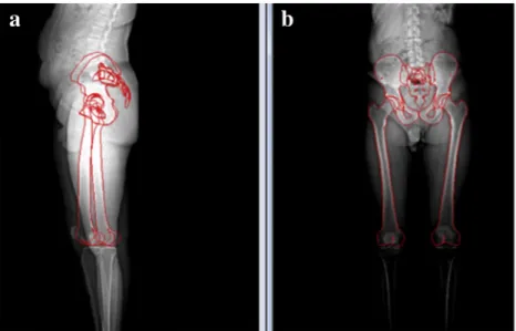
Recently, the EOS® imaging system has allowed semi-automated 3D reconstruction from two simultaneous and orthogonal size-calibrated 2D images of patients in a standing position (Figs. 1 and 2) (Dubousset et al., 2005, 2007, 2008; Rungprai et al., 2014). The main advantages of this technique are the relatively fast and easy calculation of many morphological and positional parameters due to the validated parameter-based reconstruction method (Chaibi et al., 2012; Mitton et al., 2006; Quijano et al., 2013), as well as its low irradiation, which is 6–9 times lower than conventional radiography (Chaibi et al., 2012; Deschênes et al., 2010; Quijano et al., 2013). The EOS® system addresses the limitations of CT and MRI by providing whole-body imaging, in weight-bearing, with low dose, with an acquisition time less than 20 s and parameter reconstruction times less than 10 min. It addresses the limitations of conventional 2D radiography by having simultaneous biplanar views, allowing out-of-plane parameters such as femoral torsion and pelvic rotation to be measured using the 3D model.

To the authors' knowledge, only three studies have quantiﬁed morphological parameters in non-OA and OA subjects in the standing position (Okuda et al., 2007; Than et al., 2012; Yoshimoto et al., 2005); however each has limitations. In theﬁrst study, the non-OA group had low back pain and only the sagittal-plane pelvic parameters were evaluated; in the second study, the OA group consisted only of females with hip OA secondary to acetabular dysplasia and again only the 2D pelvic parameters were evaluated; and in the third study only the lower limb parameters were evaluated.

The objectives of the present work were therefore, to provide a 3D quantitative description of the pelvis, hip and femoral morphology and relationships in a control group of asymptomatic adults and to assess the similarities and differences with a group of osteoarthritic subjects. In addition to the present healthy vs. OA study, these data provide a baseline and reference for future studies.

2. Methods

Sixty subjects were included in the study, divided evenly between a healthy group (HG) and an osteoarthritic (OA) group (Table 1). Both hips were evaluated, leading to a total of 120 lower limbs studied. The healthy group included 14 women and 16 men, averaging 46.0 years (range, 17 to 79 years; SD = 10.9). The OA group, pre-THA, included

(4)

18 women and 12 men, averaging 59.5 years (range, 25 to 81 years, SD = 15.7). The HG inclusion criteria were: absence of OA in either hip, judged radiologically by an orthopaedic surgeon and a specialist in physical medicine and rehabilitation; no previous arthroplasty or associated pathological condition of the lumbar spine, knee or ankle; and no clinical symptoms in these areas. To avoid extraneous postural effects, the inclusion criteria were: isolated hip OA (e.g. no OA of the knee or spine judged radiologically); no contralateral hip arthroplasty; and no joint arthroplasty of any other lower limb joint. The radiological OA criteria included joint space narrowing, the presence of osteophytes, and cortical bone thickening. Of the OA group, 17 had bilateral hip OA; the remaining 13 had unilateral hip OA (Table 1). The contralateral hip of the unilateral patients was not put into the healthy group since the pelvis, and possibly other joints, are still affected by the hip with OA. The effect of combining these groups was checked during the analysis. Our institutional review board approved the study.

Standing biplanar EOS® radiographs were obtained using a previ-ously published protocol (Lazennec et al., 2011b), with the subject standing comfortably and with the elbows fully ﬂexed. A 3D reconstruction was performed using previously described algorithms

(Baudoin et al., 2008; Chaibi et al., 2012; Quijano et al., 2013) and

validated for accuracy and reproducibility. The operator, a clinician specialized in neuro-orthopaedics, was trained for the reconstruction method. An expert orthopaedic surgeon selected the parameters to study based on their clinical relevance.

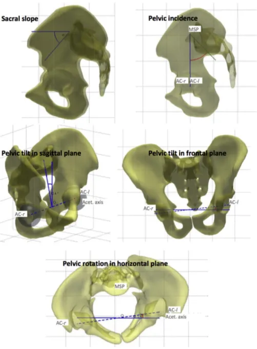
Pelvic reconstructions provided the following classical parameters (Fig. 3): sacral slope (SS), pelvic incidence (PI), sagittal pelvic tilt (PTs), frontal pelvic tilt (PTf) and horizontal pelvic rotation (PR)

(Dubousset et al., 2007, 2008; Duval-Beaupere et al., 2002; Legaye and

Duval-Beaupère, 2005; Vialle et al., 2005).

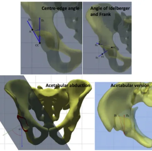
Acetabular parameters (Fig. 4) were: centre-edge angle (CEA), indicating the superior coverage of the femoral head; acetabular angle

of Idelberger and Frank (AIF), indicating acetabular depth (Tönnis, 1976); acetabular abduction (AA) (Stem et al., 2006) and acetabular version (AV) (Zilber et al., 2004).

Femoral parameters (Fig. 5) were: femoral length (L-FEM) (Strecker

et al., 1997), femoral head diameter (FHD), femoral mechanical angle

(FMA) (Yoshioka et al., 1987), hip_{–knee–shaft (HKS) angle, neck–} shaft angle (CCD angle) (Cooke et al., 1991), femoral head eccentricity (FHE), and femoral torsion (FT), each calculated in 3D.

Comparisons between the HG and OA groups, as well as the right and left hips, were performed using Student's t-tests for unpaired data, unequal variance, with significance set at P b 0.05. Although this is not the most conservative approach statistically due to the multiple comparisons, our goal was to identify potential differences or similari-ties warranting further study rather than to claim population results from this study. In cases where no significant difference was found, the sample size required to achieve 80% power was calculated and reported (assuming alpha = 0.05, a two-sided test and the worst-case standard deviation). If a large sample size (e.g. NN 100) is required to detect a difference, the difference is unlikely to be clinically significant. Correlations were calculated between each parameter to explore morphological relationships, with correlations above ρ = 0.63 highlighted (Pb 0.005); this threshold was chosen such that the param-eter explained more than 40% (i.e. 0.632_{) of the univariate variation,}

suggestive of a cause and effect relationship and potential clinical signiﬁcance. Our further goal is to provide researchers with a basis for future comparisons of these two groups, as well as a baseline for future longitudinal and post-surgery studies.

3. Results

Both the similarities and differences between the healthy and OA groups are revealing. The distributions of individual results demonstrate a wide range of individual proﬁles distinct from the group proﬁles.

Statistically signiﬁcant differences were seen between the healthy and osteoarthritic groups in the sacral slope, acetabular abduction, acetabular angle of Idelberger and Frank, femoral head eccentricity, and femoral mechanical axis angle (Pb 0.05) (Tables 2–4) (Fig. 6), as detailed below. Right–left differences were larger in the OA group compared to the healthy group for the centre-edge angle and femoral

Fig. 2. Patient-speciﬁc, parametric, 3D bone models ﬁt to EOS® images. The complex three-dimensional nature of the bones can be seen. Including the third dimension improves parameter accuracy over 2D projection-based imaging measurements.

Table 1

Demographics of the study groups.

Mean age Age range SD Sex Side Healthy (n = 30) 46.0 17–79 12.4 14F/16M – OA (n = 30) 59.5 25–81 15.6 18F/2M 18B/7R/5L

(5)

head diameter (Pb 0.05). The remaining parameters did not show statistically significant differences, which are equally important, as this shows that they are not related to the cause or effect of the disease. Pelvic incidence and the hip–knee–shaft angle parameters may have been underpowered since to detect a significant difference with 80% power would require a sample size of only 60 subjects in each group. Some subjects in both groups had numerous high or low values whereas others had only a few. The histograms (Fig. 6) reveal the surprising lack of distinction between many of the healthy and OA subjects, and the fact that the group differences are primarily defined by the high/low values. (SeeTable 5.)

Sacral slope for the OA group was almost 5° higher on average than for the healthy group (mean, 42.3° vs. 37.6°) (P = 0.04), although both had large ranges (31–64° vs. 22–64°, respectively).

The acetabulum was slightly more closed, i.e. more horizontal, in the OA group (AA = 53.2° vs. 55.0° in HG) (P = 0.02), with a similar upper limit but lower limit (43–63° vs. 49–63°).

AIF was higher in the OA group compared to the healthy group (52.3° vs. 50.8°) (P = 0.007), indicating a shallower acetabular socket, with comparable ranges of values (48–59° vs. 46–56°, respectively).

Femoral mechanical axis angle was only 1° higher in the OA group, but this was signiﬁcantly higher than the healthy group (93.0° vs. 92.0°) due to the number of high values (P = 0.02). The spread of the OA values was greater than for the HG values (88–97° vs. 84–98°).

Femoral head eccentricity showed a clear difference between the OA and healthy groups, with the OA group having 38% greater eccentricity compared to the healthy group (P = 0.003) (4.4 mm on average versus 3.2 mm), although a large range is still apparent in both groups (0.8– 11.3 mm OA vs. 0.8–7.3 mm healthy).

Left/right asymmetries existed in both the healthy and OA groups, with asymmetry being greater in the OA group for CEA (P = 0.03) and FHD (Pb 0.001). There was not a consistent difference between the bi-lateral and unibi-lateral OA subjects compared to the healthy subjects, therefore all OA subjects were considered together.

Fig. 3. Pelvic parameters, including sacral slope (SS), pelvic incidence (PI), pelvic tilt in the sagittal plane (PT-s), pelvic tilt in the frontal plane (PT-f) and pelvic rotation in the horizontal plane (PR). SS is the angle of the sacral plateau relative to the horizontal. PI is the angle between the perpendicular to the sacral slope and the line connecting the midpoint of the sacral plateau (MSP) to the acetabular centre (vertical here; may also be forward or back from vertical). PT-s is the angle between the line connecting the midpoint of the sacral plateau and the midpoint between the two acetabular centres (AC-r and AC-l). In two dimensions, PI = SS + PT-s. PT-f is the angle from the line connecting the acetabular centres (inter-acetabular line) to the horizontal; positive is tilting to the left (patient's right). PR is the angle from the inter-acetabular line to the EOS® frontal plane.

(6)

Similar relationships between parameters were seen in both groups. Right–left sides were correlated to varying amounts, with only femoral length correlated well enough to be predictive of the opposite side (HG/OA = L-FEM: 0.99/0.98; CEA: 0.59/0.65; AIF: 0.37/0.31;

FMA: 0.29/0.44; HKS: 0.08/0.41; CCD: 0.71/0.43; FHD: 0.95/0.80; FHE: 0.59/0.65).

Other correlations, greater than the deﬁned threshold, were found for: pelvic incidence vs. sacral slope (ρ = 0.78/0.71), pelvic rotation in

Fig. 4. Acetabular parameters, including centre-edge angle (CEA), indicating superior coverage, angle of Idelberger and Frank (AIF), indicating acetabular depth, acetabular abduction (AA) and acetabular version (AV). CEA is the angle between the line connecting the acetabular centre and the superior edge, with the vertical. AIF is the angle between lines D1 and D2, where D1 is the normal to the acetabular plane, passing through the acetabular centre and D2 is the line connecting where D1 intersects the acetabulum (FC) and the superior extent of the acetabulum; for example, an AIF of 45° corresponds to 100% of a hemisphere whereas an angle of 50° corresponds to only 83% of a hemisphere. AA is the angle between the normal to the acetabular plane and the vertical in 3D. AV is the angle between the plane of the acetabulum in the horizontal plane and the local sagittal (front–back) plane.

Fig. 5. Femoral parameters, including length of the femur (L-FEM), hip–knee–shaft angle (HKS), femoral mechanical angle (FMA), neck–shaft angle (CCD), diameter of the femoral head (FHD), femoral head eccentricity (FHE) and femoral torsion (FT). L-FEM is measured from the centre of the trochlear groove to the centre of the femoral head. HKS is the angle between this line and the anatomical femoral axis. FMA is the angle between the mechanical axis (L-FEM) and the distal bicondylar line. CCD is the angle between the femoral anatomical axis and the femoral neck axis. FHD is determined from a least squares sphere-ﬁt to the femoral head. FHE is the distance between the centre of the acetabular sphere and the centre of the femoral head sphere, both with a least-squaresﬁt. FT is calculated as the angle between the femoral neck and the distal bicondylar axis, projected onto the plane normal to the distal condyles.

(7)

the frontal plane vs. difference in femoral length (ρ = −0.79/−0.72), pelvic tilt vs. pelvic inclination (ρ = 0.64/0.62), and acetabular version vs. pelvic tilt (ρ = 0.63/0.69). No correlations greater than 0.1 were found for age; in other words, age accounted for less than 1% of the variation of any parameter.

4. Discussion

In this study, we quantitatively evaluated the hip, pelvis and femoral parameters in the standing position in patients with osteoarthritic and healthy hips. Although signiﬁcant differences exist between the two

Table 2

Pelvic parameters for healthy and osteoarthritic groups.

Healthy group Mean/range/SD Osteoarthritis group Mean/range/SD P-value HG vs. OA

Sample size for 80% power

Pelvic incidence (PI) 52.1° (29.0° to 75.6°) SD = 11.9° 56.3° (35.1° to 81.4°) SD = 11.5° 0.17 N = 59 Sacral slope (SS) 37.6° (22.4° to 63.6°) SD = 9.3° 42.3° (30.9° to 63.5°) SD = 8.5° 0.04 Signiﬁcant at N = 30

Pelvic tilt in the sagittal plane (PTs) 14.7°

(−4.0° to 28.8°) SD = 7.3° 14.3° (−2.7° to 32.5°) SD = 7.9° 0.86 N = 3062

Pelvic tilt in the frontal plane (PTf) 0.5°

(−3.7° to 3.4°) SD = 1.8° 0.5° (−4.3° to 3.8°) SD = 2.0° 0.57 N = inﬁnite

Pelvic rotation in the horizontal plane (PR) −0.1° (−6.5° to 6.7°) SD = 2.9° −0.8° (−15.9° to 5.4°) SD = 4.2° 0.42 N = 283 Table 3

Acetabular parameter for healthy and osteoarthritic groups. Healthy group Mean/range/SD Osteoarthritis group Mean/range/SD P-value HG vs. OA

Right Left Right Left

Centre-edge angle (CEA) 33.0° (26.1° to 47.8°) SD = 5.3° 33.0° (22.7° to 41.3°) SD = 4.6° 33.9° (19.2° to 52.9°) SD = 8.8° 33.6° (11.8° to 49.2°) SD = 8.8° 0.58 N = 950

Angle of Idelberger and Frank (AIF) 51.9° (4.7° to 56.9°) SD = 2.5° 50.8° (45.8° to 56.2°) SD = 2.6° 53.1° (46.0° to 58.5°) SD = 3.1° 52.3° (48.1° to 59.2°) SD = 2.7° 0.007 Signiﬁcant at N = 30

Acetabular abduction (AA) 54.4° (48.6° to 60.1°) SD = 3.1° 55.6° (48.5° to 62.5°) SD = 3.8° 52.7° (44.6° to 60.5°) SD = 4.3° 53.6° (43.4° to 63.3°) SD = 5.0° 0.02 Signiﬁcant at N = 30

Acetabular anteversion (AV) 18.4° (8.5° to 27.4°) SD = 4.5° 18.9° (5.5° to 26.4°) SD = 5.0° 18.1° (3.3° to 30.9°) SD = 5.6° 17.8° (6.4° to 29.8°) SD = 5.5° 0.48 N = 503 Table 4

Femoral parameter for healthy and osteoarthritic groups. Healthy group Mean/range/SD Osteoarthritis group Mean/range/SD P-value HG vs. OA

Right Left Right Left

Length of the femur (L-FEM) 423 mm (351 to 463 mm) SD = 28 mm 423 mm (352 to 460 mm) SD = 28 mm 418 mm (369 to 513 mm) SD = 31 mm 417 mm (366 to 517 mm) SD = 32 mm 0.60 N = 322

Femoral head diameter (FHD) 45.4 mm (38.2 to 51.2 mm) SD = 3.7 mm 45.1 mm (37.6 to 52.2 mm) SD = 3.6 mm 45.8 mm (40.4 to 53.5 mm) SD = 4.0 mm 45.2 mm (39.4 to 55.2 mm) SD = 4.1 mm 0.68 N = 1466

Femoral mechanical angle (FMA) 92.0° (88.2° to 95.6°) SD = 1.8° 92.0° (89.3° to 96.6°) SD = 1.9° 93.0° (84.3° to 96.8°) SD = 2.7° 92.9° (88.4° to 98.2°) SD = 2.6° 0.02 Signiﬁcant at N = 30 Hip–knee–shaft angle (HKS — 3D) 7.4° (3.5° to 1.7°) SD = 2.0° 5.6° (2.7° to 8.5°) SD = 1.1° 7.8° (4.8° to 13.2°) SD = 2.0° 6.8° (4.0° to 9.1°) SD = 1.2° 0.10 N = 50

Femoral head eccentricity (FHE) 3.4 mm (0.8 to 7.3 mm) SD = 1.7 mm 3.1 mm (1.2 to 6.9 mm) SD = 1.4 mm 4.6 mm (1.3 to 11.3 mm) SD = 2.5 mm 4.2 mm (0.8 to 6.9 mm) SD = 1.9 mm 0.001 Signiﬁcant at N = 30 Neck–shaft angle (CCD) 128.3° (120° to 143°) SD = 5.5° 126.7° (119° to 135°) SD = 4.1° 126.3° (113° to 144°) SD = 8.4° 127.1° (117° to 141°) SD = 6.7° 0.50 N = 866 Femoral torsion (FT) 1.8° (−37.1° to 37.6°) SD = 18.0° 12.2° (−29.8° to 32.0°) SD = 13.7° 8.5° (−28.8° to 40.1°) SD = 12.9° 13.2° (−14.4° to 40.1°) SD = 12.9° 0.10 N = 186

(8)

groups, each person needs to be treated individually due to the consid-erable overlap between groups. It is important to note that there is no ‘characteristic’ healthy or osteoarthritic patient and no one subject is average in all respects. An OA subject is more likely to have higher values in the parameters identiﬁed (leading to the perception of a

characteristic proﬁle) (Fig. 6), but most subjects could numerically belong to either group.

When planning for surgery, the patient's high and low parameters should be identiﬁed and analyzed for how they could affect the clinical outcome. The faster processing time of the EOS® system allows these

Fig. 6. Histograms of parameters with statistically signiﬁcant differences: sacral slope, angle of Idelberger and Frank, acetabular abduction, femoral head eccentricity, femoral mechanical angle, and the absolute differences between right and left centre-edge angles and right and left femoral head diameters. The main purpose of these histograms is to show the individual data, demonstrating the lack of distinction between most individuals with health and osteoarthritic hips, and that group differences are primarily deﬁned by their high or low values.

(9)

data to be acquired routinely. The baseline data provided by this study provide a point of comparison.

4.1. Advantages of three-dimensional analysis

The pelvis and femur are complex three-dimensional structures. Although many clinical parameters have been developed in 2D due to the availability of radiographic images, measurement errors are introduced when there is a substantial out-of-plane component. For example: femoral torsion ranged from−37° to +40°, affecting 2D parameter calculations; the average 2D HKS was 4.3° (HG) and 5.4° (OA) compared to the 3D HKS of 6.5° and 7.3°, with even larger individ-ual differences; horizontal pelvic rotation was up to 6.7° in the HG and up to 15.9° in the OA group, likewise affecting 2D calculations; and acetabular anteversion, a key parameter for THA, cannot be determined from a 2D radiograph.

4.2. Advantages of the weight-bearing position

Weight-bearing changes the orientation of the pelvis compared to supine, which inﬂuences all of the functional acetabular angles (e.g. abduction and anteversion in the horizontal and vertical planes) as well as sacral slope. If preoperative planning is to be done on an individ-ual basis, these functional positions must be considered (Lazennec et al.,

2013; Rousseau et al., 2013). Two-dimensional imaging may be

sufﬁcient to detect most abnormalities, but the comparative ease of 3D reconstruction and associated parameter calculation makes it easier toﬂag abnormal cases and to detect abnormalities that may not have originally been considered in a simple 2D radiographic analysis.

Potential causes and consequences are explored in turn below for each of the parameters with signiﬁcant group differences.

4.3. Increase in sacral slope (SS)

The higher SS (i.e. sacrum more horizontal) in OA patients is supported by previous studies (Okuda et al., 2007; Yoshimoto et al., 2005). Although this is classically considered to be the result of hip ﬂexion contracture that reduces the angle between the femur and pelvis in the standing position, with the sacrum tilting in concert with the pelvis, our data suggest otherwise. By deﬁnition, PI = PTs+ SS, or

equivalently, SS = PI− PTs. Pelvic incidence is the individual's

geomet-ric relationship between the sacral plateau and the acetabular centre, which is roughlyﬁxed in any given individual (Lazennec et al., 2013). In our study, sacral slope was 4.7° higher on average in the OA group, with pelvic incidence 4.2° higher and sagittal pelvic tilt 0.4° lower. While the latter two were not signiﬁcantly different between groups (P = 0.17 and P = 0.84), the trend suggests that, contrary to the classi-cal description, the difference in sacral slope relates more to a difference

in the geometric parameter of pelvic incidence than to the functional parameter of pelvic tilt.

4.4. Relationships of sacral slope with pelvic incidence (PI) and sagittal pelvic tilt (PTs)

Both sacral slope and sagittal pelvic tilt correlated with pelvic inci-dence (ρ = 0.62 to 0.78), but not with each other (ρ = −0.01/0.09). Since an increase in SS has been linked to an increase in lumbar lordosis to maintain the same position and horizontality of the head and eyes (Lazennec et al., 2011b; Schuller et al., 2011; Skalli et al., 2007), and SS may be higher in an OA patient (see above), vigilance is needed when planning lumbosacral fusion in patients with hip OA since the pelvis and femur are less able to provide compensatory motion. Similar vigilance is needed when planning for hip arthroplasty since the position of the pelvis affects the functional inclination and anteversion of the acetabulum (Lazennec et al., 2011b), as also seen by the correla-tion between sagittal pelvic tilt and acetabular abduccorrela-tion (ρ = 0.63) (Lazennec et al., 2012).

4.5. Increase in angle of Idelberger and Frank (AIF) and right–left asymme-try of centre-edge acetabular angle (CEA)

The higher AIF in the OA group indicates that the acetabulum was less deep. It is not clear whether this is a cause or result of the OA. On average, there was no difference in the healthy/OA CEA values or the right/left CEA values indicating that superior coverage is similar between groups and between sides. However, the larger right–left asymmetry between HG/OA shows that some individuals had large right–left differences (max 16.1°). Therefore the contralateral hip should not be taken as the model. Right/left asymmetries were not signi_{ﬁcantly different between the bilateral and unilateral OA patients.}

4.6. Acetabular abduction (AA)

For AA, the range is more relevant than the difference between groups. Particularly low or high abduction angles could result in prosthesis impingement, which should be taken into account during planning for arthroplasty surgery.

4.7. Increase in femoral mechanical angle (FMA)

The more angled anatomical axis of the femur in the OA group should be considered when planning knee arthroplasty with degenera-tive osteoarthritis of the hip. In particular, individual anatomy should be considered due to the large range of possible values, up to 98° in this group.

Table 5

Right/left asymmetry for healthy and osteoarthritic groups. Healthy group Mean/range/SD Osteoarthritis group Mean/range/SD P-value HG vs. OA

CEA |R–L| Δ = 3.6° (0.0° to 9.3°) SD = 2.6° Δ = 5.8° (0.2° to 16.1°) SD = 4.4° 0.03⁎ Significant at N = 30 FHD |R–L| Δ = 0.8 mm (0.0 to 4.0 mm) SD = 0.8 mm Δ = 2.0 mm (0.1 to 7.5 mm) SD = 1.6 mm b0.001⁎ Significant at N = 30 |LF(R)–LF(L)| Δ = 3.8 mm (0.1 to 10.5 mm) SD = 2.8 mm Δ = 4.2 mm (0.3 to 14.8 mm) SD = 3.6 mm 0.66 N = 636 ⁎ Significant P-value.

(10)

4.8. Increase in femoral head eccentricity (FHE) and in femoral head diameter (FHD) right/left asymmetry

The increase in femoral head eccentricity is likely directly related to the degenerative nature of the disease. The cause of the difference in right/left femoral head diameters is unclear. In neither case was there any correlation with age in the healthy group (ρ = 0.06 and −0.04, respectively, i.e. negligible), indicating that the differences are due to the disease rather than natural aging. In cases where the FHE is large (e.g. maximum 11.3 mm), the impact on hip arthroplasty could be profound since there is a direct relationship with femoral leg length and offset.

4.9. Relationship between femoral length (L-FEM) and pelvic inclination in the frontal plane (PT-f)

This correlation is expected since, if one leg is shorter than the other, the frontal pelvic inclination is one of the compensatory mechanisms. Neither the length of the femur nor the right/left asymmetries differed be-tween groups, but individual differences were large, up to 14.8 mm in the OA group. This preoperative status must be considered in the planning of the prosthesis placement. The global view of the standing patient provid-ed by EOS® makes this easier.

Our average healthy parameter values were within a standard deviation of that from previous studies: pelvic (Baudoin et al., 2008; Chaibi et al., 2012; Okuda et al., 2007; Strecker et al., 1997; Yoshimoto

et al., 2005), acetabular (Fowkes et al., 2011; Lubovsky et al., 2010,

2012; Tohtz et al., 2010), and femoral: (Cooke et al., 1991; Moreland

et al., 1987; Than et al., 2012).

There are several limitations to this study. First, the number of studied cases was relatively small (30 healthy subjects and 30 OA pa-tients); although underpowered for some parameters (a sample size of 60 could be sufficient for two of the non-significant parameters), this sample size was sufficient to detect the presence or lack of trends in a number of parameters and relationships, which will help guide fu-ture studies. In the cases for which large sample sizes are required to de-tect a difference, the effect size, if any, is likely of low clinical relevance. A larger study with at least 60 subjects should be conducted. Secondly, the average age of the healthy population was lower than that of the os-teoarthritis population since the development of degenerative diseases starts at a later age, resulting in non-homogeneous groups; fortunately the lack of correlation with age of any of the parameters in either the healthy or OA groups (ρ b 0.1) suggests that this difference did not play a role in the differences between groups. Thirdly, there may be ad-ditional parameters not studied, particularly inherently 3D parameters such as femoral head sphericity, that could show important differences; these become possible to include in future studies now that routine 3D measurements are possible. The most important limitation is that it is unclear whether the differences identified developed over time in indi-viduals with OA or whether these were pre-existing, possibly contribut-ing to the development of OA. A longitudinal study to track changes within the same patients, which is planned for our healthy population, would be valuable.

5. Conclusion

This study has highlighted the similarities and differences, as well as therelationships, in hip, pelvis and femoral parameters in healthy and OA subjects in the standing position. Individual characteristics must be taken into account when planning a hip, knee or spine surgery to im-prove the clinical outcome and quality of life of the patient. The low-dose EOS® system allows these parameters to be considered globally, and provides more relevant results due to the weight-bearing on the joints, and the ability to calculatethe parameters in three-dimensions.

The signiﬁcant differences between groups are suggestive of causes or effects of disease, which should be explored further. Correlations

between key parameters suggest important inter-relationships that should be kept in mind when treating any one part of the body. Con_{ﬂict of interest}

The data collection was performed within the ANR HIPEOS project, in collaboration with the EOS Imaging Company. There was no direct ﬁnancial support for the present study.

Acknowledgements

The authors would like to thank Adrien Brusson and Pr Robain Gilberte for their statistical support as well as Lucas Vancura and Yasmina Chaibi for the origin of the software and bone parameter images.

References

Babisch, J.W., Layher, F., Amiot, L.-P., 2008. The rationale for tilt-adjusted acetabular cup navigation. J. Bone Joint Surg. Am. 90, 357–365.http://dx.doi.org/10.2106/JBJS.F. 00628.

Baudoin, A., Skalli, W., de Guise, J.A., Mitton, D., 2008. Parametric subject-speciﬁc model for in vivo 3D reconstruction using bi-planar X-rays: application to the upper femoral extremity. Med. Biol. Eng. Comput. 46, 799–805. http://dx.doi.org/10.1007/s11517-008-0353-8.

Callanan, M.C., Jarrett, B., Bragdon, C.R., Zurakowski, D., Rubash, H.E., Freiberg, A.A., Malchau, H., 2011. The John Charnley Award: risk factors for cup malpositioning: quality improvement through a joint registry at a tertiary hospital. Clin. Orthop. 469, 319–329.http://dx.doi.org/10.1007/s11999-010-1487-1.

Chaibi, Y., Cresson, T., Aubert, B., Hausselle, J., Neyret, P., Hauger, O., de Guise, J.A., Skalli, W., 2012. Fast 3D reconstruction of the lower limb using a parametric model and statistical inferences and clinical measurements calculation from biplanar X-rays. Comput. Methods Biomech. Biomed. Eng. 15, 457–466.http://dx.doi.org/10.1080/ 10255842.2010.540758.

Cooke, T.D., Scudamore, R.A., Bryant, J.T., Sorbie, C., Siu, D., Fisher, B., 1991.A quantitative approach to radiography of the lower limb. Principles and applications. J. Bone Joint Surg. (Br.) 73, 715–720.

DeFrances, C.J., Hall, M.J., 2007.2005 National Hospital Discharge Survey. Adv. Data 1–19.

Deschênes, S., Charron, G., Beaudoin, G., Labelle, H., Dubois, J., Miron, M.-C., Parent, S., 2010. Diagnostic imaging of spinal deformities: reducing patients radiation dose with a new slot-scanning X-ray imager. Spine 35, 989–994.http://dx.doi.org/10. 1097/BRS.0b013e3181bdcaa4.

Dubousset, J., Charpak, G., Dorion, I., Skalli, W., Lavaste, F., Deguise, J., Kalifa, G., Ferey, S., 2005.A new 2D and 3D imaging approach to musculoskeletal physiology and pathology with low-dose radiation and the standing position: the EOS system. Bull. Acad. Natl Med. 189, 287–297 (discussion 297–300).

Dubousset, J., Charpak, G., Skalli, W., Kalifa, G., Lazennec, J.-Y., 2007.EOS stereo-radiography system: whole-body simultaneous anteroposterior and lateral radiographs with very low radiation dose. Rev. Chir. Orthop. Reparatrice Appar. Mot. 93, 141–143.

Dubousset, J., Charpak, G., Skalli, W., de Guise, J., Kalifa, G., Wicart, P., 2008. Skeletal and spinal imaging with EOS system. Arch. Pediatr. 15, 665–666.http://dx.doi.org/10. 1016/S0929-693X(08)71868-2.

Duval-Beaupère, G., Schmidt, C., Cosson, P., 1992.A Barycentremetric study of the sagittal shape of spine and pelvis: the conditions required for an economic standing position. Ann. Biomed. Eng. 20, 451–462.

Duval-Beaupere, G., Marty, C., Barthel, F., Boiseaubert, B., Boulay, C., Commard, M.C., Coudert, V., Cosson, P., Descamps, H., Hecquet, J., Khoury, N., Legaye, J., Marpeau, M., Montigny, J.P., Mouilleseaux, B., Robin, G., Schmitt, C., Tardieu, C., Tassin, J.L., Touzeau, C., 2002.Sagittal proﬁle of the spine prominent part of the pelvis. Stud. Health Technol. Inform. 88, 47–64.

Fowkes, L.A., Petridou, E., Zagorski, C., Karuppiah, A., Toms, A.P., 2011. Deﬁning a reference range of acetabular inclination and center-edge angle of the hip in asymptomatic individuals. Skelet. Radiol. 40, 1427–1434. http://dx.doi.org/10.1007/s00256-011-1109-3.

Huda, W., 2007. Radiation doses and risks in chest computed tomography examinations. Proc. Am. Thorac. Soc. 4, 316–320.http://dx.doi.org/10.1513/pats.200611-172HT. Kim, J.S., Park, T.S., Park, S.B., Kim, J.S., Kim, I.Y., Kim, S.I., 2000.Measurement of femoral

neck anteversion in 3D. Part 2: 3D modelling method. Med. Biol. Eng. Comput. 38, 610–616.

Lazennec, J.-Y., Charlot, N., Gorin, M., Roger, B., Arafati, N., Bissery, A., Saillant, G., 2004. Hip–spine relationship: a radio-anatomical study for optimization in acetabular cup positioning. Surg. Radiol. Anat. 26, 136–144. http://dx.doi.org/10.1007/s00276-003-0195-x.

Lazennec, J.-Y., Boyer, P., Gorin, M., Catonné, Y., Rousseau, M.A., 2011a. Acetabular anteversion with CT in supine, simulated standing, and sitting positions in a THA patient population. Clin. Orthop. 469, 1103–1109. http://dx.doi.org/10.1007/ s11999-010-1732-7.

Lazennec, J.-Y., Brusson, A., Rousseau, M.-A., 2011b. Hip–spine relations and sagittal balance clinical consequences. Eur. Spine J. 20, 686–698.http://dx.doi.org/10.1007/ s00586-011-1937-9.

(11)

Lazennec, J.Y., Brusson, A., Rousseau, M.-A., 2012. THA patients in standing and sitting positions: a prospective evaluation using the low-dose“full-body” EOS® imaging system. Semin. Arthroplast. 23, 220–225.http://dx.doi.org/10.1053/j.sart.2013.01. 005.

Lazennec, J.Y., Brusson, A., Rousseau, M.A., 2013. Lumbar-pelvic-femoral balance on sitting and standing lateral radiographs. Orthop. Traumatol. Surg. Res. 99, S87–S103.

http://dx.doi.org/10.1016/j.otsr.2012.12.003.

Legaye, J., Duval-Beaupère, G., 2005.Sagittal plane alignment of the spine and gravity: a radiological and clinical evaluation. Acta Orthop. Belg. 71, 213–220.

Legaye, J., Duval-Beaupère, G., Hecquet, J., Marty, C., 1998.Pelvic incidence: a fundamental pelvic parameter for three-dimensional regulation of spinal sagittal curves. Eur. Spine J. 7, 99–103.

Lubovsky, O., Peleg, E., Joskowicz, L., Liebergall, M., Khoury, A., 2010. Acetabular orientation variability and symmetry based on CT scans of adults. Int. J. Comput. Assist. Radiol. Surg. 5, 449–454.http://dx.doi.org/10.1007/s11548-010-0521-9.

Lubovsky, O., Wright, D., Hardisty, M., Kiss, A., Kreder, H., Whyne, C., 2012. Acetabular orientation: anatomical and functional measurement. Int. J. Comput. Assist. Radiol. Surg. 7, 233–240.http://dx.doi.org/10.1007/s11548-011-0648-3.

Mahaisavariya, B., Sitthiseripratip, K., Tongdee, T., Bohez, E.L., Vander Sloten, J., Oris, P., 2002. Morphological study of the proximal femur: a new method of geometrical assessment using 3-dimensional reverse engineering. Med. Eng. Phys. 24, 617–622.

http://dx.doi.org/10.1016/S1350-4533(02)00113-3.

Mitton, D1., Deschênes, S., Laporte, S., Godbout, B., Bertrand, S., de Guise, J.A., Skalli, W., 2006.3D reconstruction of the pelvis from bi-planar radiography. Comput. Methods Biomech. Biomed. Eng. 9 (1), 1–5 (Feb).

Moreland, J.R., Bassett, L.W., Hanker, G.J., 1987.Radiographic analysis of the axial alignment of the lower extremity. J. Bone Joint Surg. Am. 69, 745–749.

Okuda, T., Fujita, T., Kaneuji, A., Miaki, K., Yasuda, Y., Matsumoto, T., 2007. Stage-speciﬁc sagittal spinopelvic alignment changes in osteoarthritis of the hip secondary to developmental hip dysplasia. Spine 32, E816–E819.http://dx.doi.org/10.1097/BRS. 0b013e31815ce695.

Polkowski, G.G., Nunley, R.M., Ruh, E.L., Williams, B.M., Barrack, R.L., 2012. Does standing affect acetabular component inclination and version after THA? Clin. Orthop. 470, 2988–2994.http://dx.doi.org/10.1007/s11999-012-2391-7.

Quijano, S., Serrurier, A., Aubert, B., Laporte, S., Thoreux, P., Skalli, W., 2013. Three-dimensional reconstruction of the lower limb from biplanar calibrated radiographs. Med. Eng. Phys.http://dx.doi.org/10.1016/j.medengphy.2013.07.002.

Robertsson, O., Dunbar, M., Pehrsson, T., Knutson, K., Lidgren, L., 2000. Patient satisfaction after knee arthroplasty: a report on 27,372 knees operated on between 1981 and 1995 in Sweden. Acta Orthop. Scand. 71, 262–267.http://dx.doi.org/10.1080/ 000164700317411852.

Rousseau, M.-A., Brusson, A., Lazennec, J.-Y., 2013. Assessment of the axial rotation of the pelvis with the EOS(®) imaging system: intra- and inter-observer reproducibility and accuracy study. Eur. J. Orthop. Surg. Traumatol. http://dx.doi.org/10.1007/s00590-013-1281-3.

Rungprai, C., Goetz, J.E., Arunakul, M., Gao, Y., Femino, J.E., Amendola, A., Phisitkul, P., 2014. Foot and ankle radiographic parameters: validation and reproducibility with a biplanar imaging system versus conventional radiography. Foot Ankle Int. 35 (11), 1166–1175.http://dx.doi.org/10.1177/1071100714545514.

Schuller, S., Charles, Y.P., Steib, J.-P., 2011. Sagittal spinopelvic alignment and body mass index in patients with degenerative spondylolisthesis. Eur. Spine J. 20, 713–719.

http://dx.doi.org/10.1007/s00586-010-1640-2.

Skalli, W., Champain, S., Mosnier, T., 2007. Biomécanique du rachis [WWW Document]. URL,

http://www.reedoc-irr.fr/Record.htm?idlist=1&record=19341489124911696619

(accessed 2.10.14).

Stem, E.S., O'Connor, M.I., Kransdorf, M.J., Crook, J., 2006. Computed tomography analysis of acetabular anteversion and abduction. Skelet. Radiol. 35, 385–389.http://dx.doi. org/10.1007/s00256-006-0086-4.

Strecker, W., Keppler, P., Gebhard, F., Kinzl, L., 1997.Length and torsion of the lower limb. J. Bone Joint Surg. (Br.) 79, 1019–1023.

Subburaj, K., Ravi, B., Agarwal, M., 2009. Automated identiﬁcation of anatomical landmarks on 3D bone models reconstructed from CT scan images. Comput. Med. Imaging Graph. 33, 359–368.http://dx.doi.org/10.1016/j.compmedimag.2009.03.001. Than, P., Szuper, K., Somoskeöy, S., Warta, V., Illés, T., 2012. Geometrical values of the normal and arthritic hip and knee detected with the EOS imaging system. Int. Orthop. 36, 1291–1297.http://dx.doi.org/10.1007/s00264-011-1403-7.

Tohtz, S.W., Sassy, D., Matziolis, G., Preininger, B., Perka, C., Hasart, O., 2010. CT evaluation of native acetabular orientation and localization: sex-speciﬁc data comparison on 336 hip joints. Technol. Health Care 18, 129–136.http://dx.doi.org/10.3233/THC-2010-0575. Tönnis, D., 1976.Normal values of the hip joint for the evaluation of X-rays in children

and adults. Clin. Orthop. 39–47.

Vialle, R., Levassor, N., Rillardon, L., Templier, A., Skalli, W., Guigui, P., 2005. Radiographic analysis of the sagittal alignment and balance of the spine in asymptomatic subjects. J. Bone Joint Surg. Am. 87, 260–267.http://dx.doi.org/10.2106/JBJS.D.02043. Yoshimoto, H., Sato, S., Masuda, T., Kanno, T., Shundo, M., Hyakumachi, T., Yanagibashi, Y.,

2005.Spinopelvic alignment in patients with osteoarthrosis of the hip: a radiographic comparison to patients with low back pain. Spine 30, 1650–1657.

Yoshioka, Y., Siu, D., Cooke, T.D., 1987.The anatomy and functional axes of the femur. J. Bone Joint Surg. Am. 69, 873–880.

Zilber, S., Lazennec, J.Y., Gorin, M., Saillant, G., 2004. Variations of caudal, central, and cranial acetabular anteversion according to the tilt of the pelvis. Surg. Radiol. Anat. 26, 462–465.http://dx.doi.org/10.1007/s00276-004-0254-y.