Prediction of necking in thin sheet metals using an elastic‒plastic model coupled with ductile damage and bifurcation criteria

Science Arts & Métiers (SAM)

is an open access repository that collects the work of Arts et Métiers Institute of Technology researchers and makes it freely available over the web where possible.

This is an author-deposited version published in: https://sam.ensam.eu Handle ID: .http://hdl.handle.net/10985/17483

To cite this version :

Yasser BOUKTIR, Hocine CHALAL, Farid ABED-MERAIM - Prediction of necking in thin sheet metals using an elasticplastic model coupled with ductile damage and bifurcation criteria -International Journal of Damage Mechanics - Vol. 27, n°6, p.801–839 - 2018

Any correspondence concerning this service should be sent to the repository Administrator : archiveouverte@ensam.eu

1

Prediction of necking in thin sheet metals using an

elastic‒plastic model coupled with ductile damage and

bifurcation criteria

Yasser Bouktir 1,2, Hocine Chalal 1,3 and Farid Abed-Meraim 1,3,*

1

Laboratoire d'Étude des Microstructures et de Mécanique des Matériaux, LEM3, UMR CNRS 7239, Arts et Métiers ParisTech, 4 rue Augustin Fresnel, 57078 Metz

Cedex 3, France 2

Laboratoire Procédés de Fabrication, LPF, École Militaire Polytechnique, Bordj El Bahri, 16046, Algérie

3

Laboratory of Excellence on Design of Alloy Metals for low-mAss Structures, DAMAS, Université de Lorraine, France

Abstract

In this paper, the conditions for the occurrence of diffuse and localized necking in thin sheet metals are investigated. The prediction of these necking phenomena is undertaken using an elastic‒plastic model coupled with ductile damage, which is then combined with various plastic instability criteria based on bifurcation theory. The bifurcation criteria are first formulated within a general three-dimensional modeling framework, and then specialized to the particular case of plane-stress conditions. Some theoretical relationships or links between the different investigated bifurcation criteria are established, which allows a hierarchical classification in terms of their conservative character in predicting critical necking strains. The resulting numerical tool is implemented into the finite element code ABAQUS/Standard to predict forming limit diagrams (FLDs), in both situations of a fully three-dimensional formulation and a plane-stress framework. The proposed approach is then applied to the prediction of

2 diffuse and localized necking for a DC06 mild steel material. The predicted FLDs confirm the above-established theoretical classification, revealing that the general bifurcation criterion provides a lower bound for diffuse necking prediction, while the loss of ellipticity criterion represents an upper bound for localized necking prediction. Some numerical aspects related to the prestrain effect on the development of necking are also investigated, which demonstrates the capability of the present approach in capturing the strain-path changes commonly encountered in complex sheet metal forming operations.

Keywords

Stability and bifurcation, Ductility, Constitutive behavior, Elastic‒plastic material, Forming limit diagrams

* Corresponding author: F Abed-Meraim

Tel.: +(33) 3.87.37.54.79; fax: +(33) 3.87.37.54.70.

3

Introduction

During sheet metal forming processes, various types of defects related to operating conditions and/or material characteristics may occur. Among them, plastic instabilities associated with the occurrence of diffuse and localized necking are particularly detrimental, since they limit sheet metal formability. In this context, Keeler and Backofen (1963) and Goodwin (1968) proposed the nowadays well-known concept of Forming Limit Diagram (FLD), to characterize the formability of thin sheet metals subjected to in-plane stretching. The determination of FLDs was originally based on experimental measurements, which turned out to be very time consuming and entailing non-negligible costs, not to mention their potential lack of reproducibility. To overcome these drawbacks, significant efforts have been devoted over the last decades to the development of theoretical indicators that are able to predict the formability limits of thin sheet metals. To this end, a complete approach to the prediction of critical limit strains requires essentially two developments. The first consists of an advanced constitutive model capable of reproducing the essential physical phenomena that occur during forming operations, while the second pertains to relevant criteria for the reliable prediction of plastic instabilities.

Along with the evolution of necking in sheet metal forming processes, ductile damage plays an important role with regard to the formability limits of thin sheet metals. This requires accurate modeling of the initiation of ductile damage and its evolution during loading, in order to reproduce the softening mechanisms observed experimentally at large deformations. In this field, two well-established theories of ductile damage have been developed over the past few decades. The first theory, which has been initiated by the work of Gurson (1977), and further modified by Tvergaard and Needleman (see, e.g., Tvergaard, 1981; Tvergaard and Needleman 1984), is based on a micromechanical analysis of void growth that describes the complex ductile damage

4 mechanisms in porous materials. In this approach, the void volume fraction is introduced as damage variable, thus accounting for the dependence of the material response on hydrostatic pressure. Several improvements have been made in the literature to this type of ductile damage theory, but at the expense of a large number of material parameters (see, e.g., Rousselier, 1987; Gologanu et al., 1997; Pardoen et al., 1998; Benzerga and Besson, 2001; Monchiet et al., 2008). The second theory, known as continuum damage mechanics (CDM), is based on the thermodynamics of irreversible processes and is widely used for modeling ductile damage in metallic materials (see, e.g., Lemaitre, 1992; Voyiadjis and Kattan, 1992; Chaboche, 1999). In this approach, the damage variable represents the surface density of microcracks across a given plane, and can be modeled as isotropic scalar variable (see, e.g., Lemaitre, 1985, 1992; Chaboche et al., 2006), or a tensor variable for anisotropic damage (Chow and Wang, 1987; Chow and Lu, 1989; Chaboche, 1993; Zhu and Cescotto, 1995; Abu Al-Rub and Voyiadjis, 2003, Brünig, 2003). Three main variants for the CDM theory have been essentially developed in the literature, which are based on the following three fundamental assumptions: the strain equivalence principle, the stress equivalence principle and the energy equivalence principle. The strain equivalence principle employs the concept of effective stress, as proposed by Lemaitre (1971), and subsequently used by Simo and Ju (1987a, 1987b) and Ju (1989). In contrast to the strain equivalence principle, the stress equivalence principle is based on the concept of effective strain, as summarized by the works of Simo and Ju (1987a, 1987b). As to the third variant for the CDM theory, which is the elastic energy equivalence principle, it was first introduced by Cordebois and Sidoroff (1979) as an alternative to the available strain or stress equivalence principles, and extended by Saanouni and co-workers during the last decades to the total energy equivalence assumption (see, e.g., Saanouni et al., 1994, 2011; Saanouni and Chaboche, 2003; Saanouni, 2008, 2012; Saanouni and Hamed, 2013; Ghozzi et al., 2014; Rajhi et al., 2014; Yue et al., 2015; Badreddine et al.,

5 2010, 2016, 2017). This total energy equivalence principle defines the undamaged material state and its corresponding effective strain and stress variables, so that the total (elastic and inelastic) energy involved is equal to that for the damaged material state.

To predict the occurrence of diffuse or localized necking in sheet metal forming processes, the above-discussed constitutive models need to be coupled with plastic instability criteria. These criteria can be classified into four categories. The first category of criteria is based on Considère’s maximum force principle (Considère, 1885), who proposed a diffuse necking criterion in the particular case of uniaxial tension. Later, Swift (1952) extended Considère’s criterion to the case of in-plane biaxial loading. For localized necking, Hill (1952) proposed an alternative criterion based on bifurcation theory, which states that localized necking occurs along the direction of zero extension. It is worth noting that Hill’52 criterion is only applicable to the left-hand side of the FLD and, therefore, it was often combined with Swift’52 criterion to determine a complete FLD. Within the category of maximum force principle criteria, Hora et al. (1994, 1996) and Mattiasson et al. (2006) proposed two extensions of Considère’s criterion for the prediction of localized necking, which take into account the strain-path changes. The second category of criteria is based on the approach that assumes the existence of an initially inhomogeneous region, with an initial imperfection, from which localized necking may occur. The initial imperfection may take the form of geometric imperfection, which led to the so-called M‒K approach (Marciniak and Kuczyński, 1967), and was subsequently extended by Hutchinson and Neale (1978), by allowing the groove, postulated with an initial orientation, to rotate in the sheet plane, or material imperfection (see, e.g., Yamamoto, 1978). The third category of criteria is derived from bifurcation or stability theories. These criteria have sound theoretical foundations, since they investigate the possibility of bifurcation or instability in the constitutive description itself, without introducing arbitrarily

user-6 defined parameters, such as the initial imperfection size in the M‒K approach. Drucker (1950, 1956) and, later, Hill (1958) developed quite general bifurcation conditions, based on the loss of uniqueness for the solution of the associated boundary value problem, which will be referred to in the current work as the general bifurcation criterion (GB). A local formulation for the GB criterion, which corresponds to the positiveness of the second-order work, may be used for the prediction of diffuse necking in sheet metals. In the same context, Valanis (1989) proposed an alternative criterion, designated as limit-point bifurcation (LPB), which is less conservative than the GB criterion. The LPB criterion is associated with the stationarity of the first Piola‒Kirchhoff stress state, which corresponds to the singularity of the associated analytical tangent modulus. Following the pioneering works of Hill (1952, 1958, 1962), Rudnicki and Rice (1975), Stören and Rice (1975) and Rice (1976) proposed a localization bifurcation criterion to predict the localization of deformation in the form of planar shear bands or localized necking in thin metal sheets. The latter criterion corresponds to the loss of ellipticity (LE) of the partial differential equations governing the associated boundary value problem. An alternative localization criterion, more conservative than the LE criterion, was proposed by Bigoni and Hueckel (1991) and Neilsen and Schreyer (1993), which consists in the loss of strong ellipticity (LSE) of the equations governing the boundary value problem. Some other variants for the above-discussed bifurcation criteria are also worth mentioning as well as further analytical developments with the aim of deriving closed-form expressions for the critical limit strains associated with diffuse or localized necking (see, e.g., Doghri and Billardon, 1995; Loret and Rizzi, 1997a, 1997b; Rizzi and Loret, 1997; Sánchez et al., 2008). In particular, Benallal and co-workers (see, e.g., Benallal et al., 1993; Pijaudier-Cabot and Benallal, 1993; Lemaitre et al., 2009) combined the CDM theory with the bifurcation analysis for the prediction of strain localization in rate-independent materials. In these

7 works, closed-form solutions were derived for both local and nonlocal damage-based constitutive equations.

The fourth and last category of plastic instability criteria relies on the theory of stability, and the associated perturbation analysis, for the prediction of diffuse or localized necking (see, e.g., Fressengeas and Molinari, 1987; Dudzinski and Molinari, 1991; Toth et al., 1996; Boudeau, 1998). This class of criteria represents an interesting alternative to the bifurcation approach, especially in the case of strain-rate-dependent materials. However, it is noticeable that this latter approach is less commonly used in the literature, as compared to the M‒K analysis or the bifurcation theory.

In the current contribution, an elastic‒plastic model, with Hill’48 anisotropic plastic yield surface and mixed isotropic‒kinematic hardening, is coupled with the CDM theory, and more specifically, with the Lemaitre isotropic damage model. Referring to the earlier works of Benallal et al. (1993) and Doghri and Billardon (1995), who coupled the CDM theory with the LE criterion, the proposed elastic‒plastic‒damage model is combined with the above-described four bifurcation criteria to predict the occurrence of diffuse and localized necking in thin sheet metals. The resulting numerical tool is implemented into the finite element code ABAQUS/Standard, within the framework of large plastic strains and a fully three-dimensional formulation. Specially modified versions of the proposed approach are also implemented in the two particular frameworks of small strains and plane-stress conditions.

The remainder of paper is organized as follows. The constitutive equations of the fully coupled elastic‒plastic‒damage model are introduced in the next Section (i.e., second Section), along with their numerical implementation and validation. The bifurcation criteria adopted for the prediction of diffuse and localized necking are presented in the third Section, within a general modeling framework. Then, the

8 bifurcation criteria are specialized to the two particular frameworks of plane-stress conditions and small strain analysis. Also, a theoretical classification of these bifurcation criteria is established, in terms of their conservative character in predicting the critical limit strains. In the fourth Section, the numerical tool resulting from the present approach is first validated, and then applied to the prediction of FLDs for a steel material. The simulation results confirm the theoretical hierarchy previously established for the bifurcation criteria with regard to their order of prediction for the critical necking strains. Finally, the main results are summarized and conclusions are drawn.

Elasto-plastic model coupled with ductile damage

In this Section, the constitutive equations of the elastic‒plastic model coupled with ductile damage are described. This constitutive modeling is developed within the framework of phenomenological behavior laws with rate-independent associative plasticity. The damage is first introduced through an isotropic scalar variable describing the degradation of the material elasticity properties. Then, a general thermodynamic framework is used to derive the fully coupled constitutive equations under the postulate of strain equivalence principle. Finally, the implementation of the resulting fully coupled elastic‒plastic‒damage model into the finite element software ABAQUS/Standard is performed via a user-defined material (UMAT) subroutine, and validated by comparing the numerical predictions with those given by existing hardening models available in ABAQUS as well as with reference solutions taken from the literature.

9

Anisotropic elastic‒plastic model coupled with ductile damage

The concept of continuum damage mechanics (CDM) has been widely used in the literature to describe the degradation of the material mechanical properties during loading. The CDM theory was first introduced by Kachanov (1958) to model creep rupture. Subsequently, the CDM approach has been further developed and formulated within the framework of thermodynamics to model mainly three types of ductile damage: fatigue damage (Chaboche, 1974), creep damage (Rabotnov, 1963; Hult, 1974) and ductile plastic damage (see, e.g., Lemaitre, 1985; Lemaitre and Dufailly, 1977). More specifically, three damage representation theories have been developed in the literature, which are based on three fundamental assumptions; namely, the strain equivalence principle, the stress equivalence principle and the energy equivalence principle. The first class of damage representation theories, which is based on the strain equivalence principle, employs the concept of effective stress, as proposed by Lemaitre (1971), and subsequently used by Simo and Ju (1987a, 1987b) and Ju (1989). By adopting this concept, the constitutive equations of the damaged material are derived from those of the undamaged material by substituting the effective stress tensor σɶ by its expression in terms of the Cauchy stress tensor σ_{, as follows:}

1 d

= −

σ

σ_{ɶ , (1)}

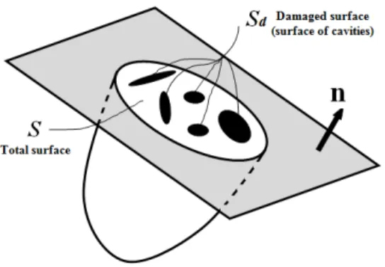
where σ _{is the Cauchy stress tensor in the damaged material, and σɶ the effective stress} tensor in an equivalent undamaged material. The scalar damage variable d , varying from 0 to 1 (with d =0 for an undamaged material, and d =1 for a fully damaged material), represents the surface density of cavities and cracks within a given plane (see Figure 1), and is defined by the following relationship:

10 1 eff d S S d S S = = − , (2)

where S is the surface of defects (cavities and cracks), _d S_eff denotes the effective surface (undamaged surface), and S is the total surface.

Figure 1. Schematic representation of a partially damaged section.

The second class of damage representation theories is based on the stress equivalence principle, as summarized by the works of Simo and Ju (1987a, 1987b), who introduced the concept of effective strain. Finally, Cordebois and Sidoroff (1979) proposed the elastic energy equivalence assumption, which assumes the equality between the elastic energy defined in the real damaged configuration and the one defined in the fictive undamaged configuration. This leads to the definition of a single couple of state variable related to the plastic flow. This idea has been extended later by Saanouni and co-workers (see, e.g., Saanouni et al., 1994, 2011; Saanouni and Chaboche, 2003; Saanouni, 2008, 2012; Saanouni and Hamed, 2013; Ghozzi et al., 2014; Rajhi et al., 2014; Yue et al., 2015; Badreddine et al., 2010, 2016, 2017) to the total energy equivalence assumption, from which a couple of effective state variables associated with each dissipative phenomenon can be defined.

11 In this subsection, the elastic−plastic constitutive equations coupled with the Lemaitre isotropic damage model are formulated within the framework of the thermodynamics of irreversible processes with state variables. The strain equivalence principle, using the concept of the effective stress, is adopted here to derive the fully coupled elastic−plastic−damage model. Assuming isothermal conditions, the Helmholtz free energy is taken as state potential, which can be additively decomposed as follows:

( )

Elastic contribution Plastic contribution

1

(1 ) : : :

2 3

e e X Csat X r

ρψ= −d ε _{C ε +} α α+ρψ r _{, (3)}

where ρ is the density, εe _{is the elastic strain tensor, and C is the fourth-order}

elasticity tensor. The second-order tensor α _{represents the back-strain internal variable,} whose associated thermodynamic force is the back-stress tensor X . The latter represents the kinematic hardening, i.e. the translation of the yield surface in the stress space, with X_sat and C being the associated material parameters. The potential _X ψr

( )

in Eq. (3) is a function of the scalar internal variable r , which represents the isotropic strain hardening. The associated thermodynamic force is the scalar variable R , which measures the size variation of the yield surface in the stress space.

The thermodynamic forces associated with each internal variable, i.e.

(

)

are derived from the state potential (see Eq. (3)) as follows: Cauchy stress tensor =ρ∂ψ_e = −

(

)

∂

σ _{C ε}

ε . (4)

Isotropic hardening stress

r ψ ψ R ρ ρ r r ∂ ∂ = = ∂ ∂ . (5)

12 Kinematic hardening stress

3 sat X ψ 2 ρ∂ X C = = ∂ X α α . (6)

Damage driving force 1 : : 2 e ψ e e Y ρ d ∂ = − = ∂ ε C ε . (7)

The above damage driving force is commonly called the “elastic strain energy density release rate”, which represents the variation of internal energy density due to damage growth at constant stress (see, e.g., Lemaitre, 1992; Lemaitre et al., 2000). It can be easily shown that, for linear isotropic elasticity, the expression of Y reduces to e

(

) (

)

J = σɶ′ ′σɶ _{is the equivalent effective stress in the sense of von Mises,}

H σ

′ = −

σɶ σɶ _{ɶ 1 is the deviatoric part of the effective stress and} 1 _:

3

H

σ_ɶ = σɶ _{1 is the}

hydrostatic effective stress, while E and υ denote, respectively, the Young modulus and Poisson ratio.

The second principle of thermodynamics, written in the form of the Clausius−Duhem inequality, must be always satisfied in order to ensure the validity of the model. In the case of isothermal processes, the Clausius−Duhem inequality writes

: −ρψ≥0

σ _{D ɺ , (9)}

where the second-order tensor D represents the strain rate, which is additively decomposed into two second-order tensors De and Dp, representing the elastic strain rate and the plastic strain rate, respectively (i.e., = e+ p

13 The free energy rate ψɺ in Eq. (9) writes

: e : e ψ ψ ψ ψ ψ r d r d ∂ ∂ ∂ ∂ = + + + ∂ε D ∂α α ∂ ∂ ɺ ɺ ɺ ɺ . (10)

Substituting the above equation in Eq. (9), and using the definition of the associated thermodynamic forces, the Clausius−Duhem inequality becomes

: p − : −R r Y d+ e ≥0

σ _{D X αɺ ɺ} ɺ _{. (11)}

In the particular case when the plastic dissipation is negligible, the following condition must be always satisfied:

0 e

Y dɺ≥ , (12)

which requires the damage rate dɺ to be positive, since Y is a positive quadratic e

function (see Eq. (7)).

Once all the state variables are defined, their evolution laws are derived from a dissipation potential F , which is a convex function of the associated thermodynamic forces. Its general form is given by

(

)

( )

where the first term F_p

(

)

3 :

4X_sat X X is related to the nonlinear part of the kinematic hardening, and the last term

( )

d

14 By applying the classical normality rule pertaining to generalized standard materials, the evolution laws are written as

p e F λ F r λ R F λ F d λ Y ∂  =  _∂  ∂  _{= −}  _∂  ∂  _{= −}  _∂  _∂  ₌ ∂  D σ α X ɺ ɺ ɺ ɺ ɺ ɺ ɺ , (14)

where λɺ is the plastic multiplier.

In this work, the plastic potential F_p in Eq. (13) is assumed to be equal to the plastic yield function, which leads to the classical associative plasticity theory. Accordingly, the plastic potential F_p can be written in the following generic form:

( , )

p

F =σ σɶ′ _X −Y _{, (15)}

where σ is the equivalent effective stress, while Y = Y + R is a measure of the size of ₀

the yield surface, with Y being the initial yield stress. ₀

The initial anisotropy of the material is taken into account here via the equivalent effective stress σ . In the literature, several plastic yield surfaces have been used to represent the plastic anisotropy of materials (see, e.g., Hill, 1948, 1990, 1993; Barlat et al., 1991; Banabic et al., 2003). In this work, the quadratic Hill’48 yield criterion is adopted for modeling the plastic anisotropy of the material. The corresponding equivalent effective stress is given by the following expression:

15

( , ) ( ) ( )

σ σɶ′ _X = σɶ′−_X : :_M σɶ′−_{X , (16)} where M is a fourth-order tensor that contains the six anisotropy coefficients of the quadratic Hill’48 yield criterion.

Using the above definitions, the plastic yield conditions, written in the form of Kuhn–Tucker inequalities, can be expressed as follows:

0 ( ) ( ) 0 0 0 p p F R Y λ λF  _{= ′− : : ′− − − ≤}  ≥   ₌  σ_{ɶ X M} σ_{ɶ X} ɺ ɺ . (17)

The plastic strain rate D , defined by Eq. (14), can be expressed in the case of p Hill’48 yield criterion as

p F λ∂ λ = = ∂ D V σ ɺ _{ɺ ɶ , (18)} where 1 ( ) 1 d σ ′ : − = − M σ _X

Vɶ ɶ is the plastic flow direction, normal to the yield surface.

Hardening evolution laws

From the evolution laws given by Eq. (14) and the definition of the plastic potential F_p

(see Eq. (15)), the evolution law for the isotropic strain hardening r is given by

F r λ λ R ∂ = − = ∂ ɺ ɺ ɺ . (19)

16 To provide the best description for the experimental stress‒strain response that characterizes the material strain-hardening behavior, several well-known hardening functions have been proposed in the literature. The most commonly used isotropic hardening laws are adopted in this work, due to their simple expressions that involve a reduced number of parameters. Table 1 provides the expressions of these classical isotropic hardening laws, as functions of the equivalent plastic strain ε , in the case of plasticity uncoupled from damage. When damage is coupled with plasticity, then the equivalent plastic strain ε in Table 1 should be replaced by λ to account for the coupling with damage. Indeed, the equivalent plastic strain rate εɺ is related to the plastic multiplier λɺ by the following relationship:

1 λ ε d = − ɺ ɺ _{, (20)}

which is derived from the plastic work equivalence principle (i.e., σ εɺ =(σɶ′ −_X) :_DP_).

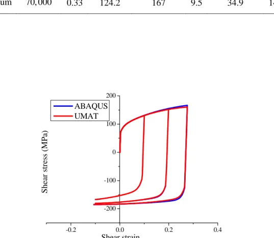
Table 1. Commonly used isotropic hardening laws. Isotropic

hardening law Hollomon Ludwig Swift Voce

Y kεn 0 n Y +kε k ε

(

)

(

)

Similarly, the evolution law for the back-strain tensor α _{is derived as}

(

)

17

(

)

where Vɶ is defined by Eq. (18). Note that the saturation direction for the back-stress variable X , whose evolution law is given by Eq. (22), coincides with that of the plastic flow direction (see Eq. (18)). However, other kinematic hardening models have been proposed in the literature, in which the saturation direction for the back-stress tensor X differs from the plastic flow direction. In particular, the well-known Armstrong−Frederick kinematic hardening law (see Armstrong and Frederick, 1966) has been originally proposed based on the following rate form (see also, e.g., Haddadi et al., 2006; Butuc et al., 2011):

(

)

nɶ ɶ is the saturation direction, which differs from the plastic flow direction given by Eq. (18). Note that in the case of the von Mises yield surface, the above saturation direction nɶ coincides with that of the plastic flow direction Vɶ . In this work, the hardening parameters as well as the Hill’48 anisotropy coefficients, used for the prediction of FLDs for a DC06 mild steel material, were experimentally identified by Haddadi et al. (2006). In the latter reference, the original Armstrong−Frederick kinematic hardening law (see Eq. (23)), together with the Swift isotropic hardening law and the Hill’48 plastic yield criterion, were considered in the identification procedure. Consequently, the nonlinear kinematic hardening law given by Eq. (23) is adopted in the current contribution. Adopting this choice, it should be noted that the evolution law given by Eq. (23) does not derive directly from the current thermodynamic approach. Nevertheless, it is very easy to slightly modify the state potential as well as the dissipation potential given by Eqs. (3) and (13), respectively, by introducing the

fourth-18 order tensor M and its inverse, so that Eq. (23) derives straightforwardly from these potentials, thus providing a consistent thermodynamic framework.

Damage evolution law

Softening behavior that takes place at large strain during loading is accounted for in this work by coupling the elastic‒plastic model with the Lemaitre ductile damage (Lemaitre, 1985). Different formulations can be found in the literature to define the damage potential for ductile materials. In this work, the following damage potential is adopted (see, e.g., Lemaitre, 1985; Saanouni et al. (2010)):

(

)

Y are the damage-related parameters, while Ye is defined by Eq. (8).

The associated damage evolution law derives from the damage potential F_d as

(

)

Elastic–plastic tangent modulus

According to the strain equivalence principle (see Eq. (1)), the Cauchy stress can be expressed using the following relationship:

19

(

)

(

)

1 d

= − : −

σ _C ε ε _{. (26)}

From the above equation, the Cauchy stress rate is derived as:

(

)

(

)

which can be rewritten in the following compact rate form:

ep

= :

σɺ _{C D, (28)}

where Cep is the elastic‒plastic tangent modulus, which is part of the ingredients required in the formulation of the bifurcation criteria developed in the next Section. In order to determine the expression of the elastic‒plastic tangent modulus Cep, the plastic multiplier λɺ needs to be first derived using the consistency condition Fɺp =0 along with

the evolution equations described in the previous Section, which writes (Haddag et al., 2009) Y λ H : : = : : + : X+ V C D V C V V H ɺ ɶ , (29)

where V =

(

)

governs the evolution of isotropic hardening (i.e., Yɺ = =Rɺ H λ_Yɺ). By combining Eqs. (18), (25), (27), and (29), Eq. (28) can be rewritten in the following form:

(

)

(

) (

)

(

)

20

[

]

(

)

Numerical implementation of the fully coupled model and its validation

Explicit time integration scheme

The resulting fully coupled model is implemented into the finite element code ABAQUS/Standard. This allows solving boundary value problems (BVP), which are governed, within the framework of isothermal processes and quasi-static analysis, by the following strong form of equilibrium equations on a given domain Ω :

( )

where ∂Ωt and ∂Ωu are complementary boundary subsurfaces of the global surface

Ω

∂ (i.e., ∂ = ∂Ω Ω_t∪∂Ω_{u and}

t u

Ω Ω

∂ ∩∂ = ∅), b is the body force vector, t is the externally-applied force vector on ∂Ω_{t, n is a unit vector normal to}

t

Ω

∂ , u is the displacement field, and ˆu is the prescribed displacement, which is applied on the boundary subsurface ∂Ω_{u. In the context of the finite element method, an alternative to}

the above strong form of equilibrium equations is the weak variational formulation, which is commonly called the principle of virtual works (PVW).

21 The constitutive equations described in the previous Section together with the weak form of the BVP allow us to derive the quasi-static finite element formulation, which is expressed here by the following set of nonlinear equations:

=

⋅

K u f , (33)

where K is the stiffness matrix, whose calculation requires the consistent tangent modulus and the discrete gradient operator of each individual finite element, while f is the generalized force vector. For each increment of the applied loading, ABAQUS/Standard solves the above system of equations iteratively using the Newton−Raphson method in order to obtain the nodal displacement vector u of the studied structure. On the other hand, the stress state as well as the consistent tangent modulus, required for setting up the global equilibrium system (see Eq. (33)), have to be computed and updated at each integration point. To achieve this, the explicit forward fourth-order Runge–Kutta integration scheme is used in this work. This choice is a reasonable compromise in terms of computational efficiency, accuracy, and convergence. However, it requires small time increments to ensure accuracy and stability (see, e.g., Li and Nemat-Nasser, 1993; Kojic, 2002).

One can notice that, for the fully coupled model, the evolution of all internal variables can be written in the form of the following global differential equation:

( )

= y

yɺ h y , (34)

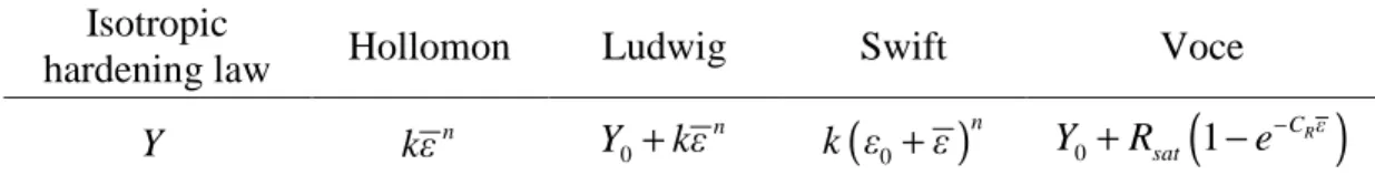
where vector y includes all internal variables of the present model. The implementation of this compact form, using the fourth-order Runge–Kutta explicit time integration scheme, is straightforward and allows incorporating various hardening laws and plastic yield surfaces (see Mansouri et al. (2014) for more details). The resulting explicit time integration algorithm is summarized in Table 2.

22 Note that, within the large strain framework, the use of objective derivatives for the tensorial variables is required in order to ensure the incremental objectivity of the model. Several objective rates have been developed in the literature, which allow simplifying the time derivatives of the constitutive equations, thus making them identical in form to a small-strain formulation. Another convenient way, which is quite equivalent to the use of objective rates, is the formulation and time integration of the constitutive equations in the so-called local objective frames. Different objective local frames have been proposed; one possible choice is the co-rotational frame associated with the anti-symmetric part W of the velocity gradient G , resulting in the conventional Jaumann rate. Another choice has been suggested by the polar decomposition theorem for the deformation gradient: F=V R , where V is the left ⋅ stretch tensor and R is the rotation tensor, which leads to the objective derivative of Green−Naghdi. The goal of such objective derivatives is to satisfy the material invariance by eliminating all the rotations that do not contribute to the material response.

Although the co-rotational Jaumann rate is the most commonly-used objective derivative, it has some well-recognized drawbacks. The main downside that has been pointed out in the use of the Jaumann rate consists of undesirable oscillations in the shear stress−strain response, as a result of large rotation of the stress principle axes, in particular when kinematic hardening is considered (see, e.g., Dafalias, 1985). It must be noted, however, that in the current work, only in-plane biaxial loading paths are considered for the prediction of conventional FLDs for sheet metals, which excludes the occurrence of shear strains during the simulations. Moreover, the limit strains expected from the application of the present bifurcation criteria, which correspond to the occurrence of diffuse or localized necking, are relatively small when compared to the large strains that sheet metals can undergo before fracture. Consequently, the Jaumann

23 rate is adopted in this work to describe the rotation of the material frame, which is consistent with the choice adopted in the ABAQUS software.

Table 2. Outline of the explicit time integration algorithm. For t = 0 , initialization of the state variables y₀ =0 Input data: ∆ε and y_n

(

)

Set ∆σ0 =0 and ∆y0 =0

For i=1,...,N (with N =4 for the 4th-order Runge–Kutta method) Compute σi =σn+ ∆ai σi−1 and yi =yn+ ∆ai yi−1, with

1 1 = 0, , ,1 2 2       a

• Plastic yield condition: if

(

)

i

p i i i

F σɶ′ _X R < _{then (elastic loading)}

(

)

i di

∆ = −σ _C ∆ε_,

i

∆ =y 0 , C_ialg = −

(

)

• Else, if ∆ε:_Vɶ_i < 0 _{then (elastic unloading)}

Apply the same treatment as in the previous operation

• Otherwise (plastic loading)

(

)

λ

(

)

(

)

(

)

(

)

Update stress and state variables

1 1 = + N n n i i i b + = ∆

∑

∑

1 = N alg alg i i i b =

∑

24

Numerical validation

The constitutive equations of the above elastic‒plastic‒damage model have been implemented into the finite element code ABAQUS/Standard, within the framework of large strains and a three-dimensional formulation. The numerical validation of this finite element implementation of the model is conducted stepwise in this subsection. In a first step, the numerical implementation of the elastic‒plastic model alone (i.e., without coupling with damage) is preliminarily validated through various classical tests.

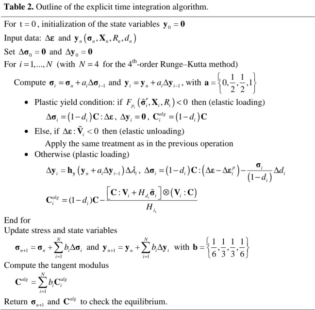
The first numerical simulations consist of Bauschinger shear tests. The latter allow validating the nonlinear hardening behavior, which is described by the combined isotropic and kinematic hardening model. More specifically, the combined hardening model based on the Voce isotropic hardening law and the Armstrong–Frederick kinematic hardening law, together with the von Mises yield criterion, is used in this simulation, which allows comparing the numerical results with those obtained using the same combined hardening model available in the ABAQUS software. The associated elasticity and hardening parameters, which correspond to a standard aluminum material, are summarized in Table 3. Three Bauschinger shear tests are simulated as follows: three different amounts of shear strain, i.e. 0.1, 0.2 and 0.3, are first prescribed to the studied aluminum material, then followed by a reverse shear loading path up to a shear strain of ‒0.1. Figure 2 reports the simulated shear stress−strain curves obtained with the developed UMAT subroutine and the built-in ABAQUS model. These comparisons with the reference results given by ABAQUS reveal the good accuracy of the developed integration algorithm in the case of combined nonlinear hardening model.

Table 3. Elasticity and hardening material parameters used for the simulations. Material E(MPa) υ Y0(MPa) Rsat(MPa) CR Xsat(MPa) CX

25 Aluminum 70, 000 0.33 124.2 167 9.5 34.9 146.5 -0.2 0.0 0.2 0.4 -200 -100 0 100 200 S h ea r st re ss ( M P a) Shear strain ABAQUS UMAT

Figure 2. Shear stress−strain curves obtained with the developed UMAT subroutine and the built-in ABAQUS model.

In order to evaluate the accuracy of the numerical implementation of the anisotropic behavior, which is based on the Hill’48 yield criterion, simulations of classical uniaxial tensile tests at 0°, 45° and 90° from the rolling direction are performed here. To achieve this, the aluminum material presented in the previous validation tests is used here with the Hill’48 yield criterion. The corresponding anisotropy coefficients are reported in Table 4. It is worth noting that the description of plastic anisotropy available in ABAQUS, which is based on the Hill’48 yield criterion, can only be combined with

26 isotropic hardening. Accordingly, to allow consistent comparisons, only the Voce isotropic hardening model is used in the current simulations of uniaxial tensile tests at different orientations from the rolling direction. In addition to the anisotropy coefficients given in Table 4, the elasticity and Voce hardening parameters used in these simulations are taken from Table 3.

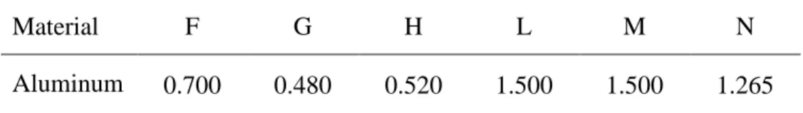
Table 4. Hill’48 anisotropy coefficients for the studied aluminum material.

Material F G H L M N

Aluminum 0.700 0.480 0.520 1.500 1.500 1.265

Figure 3 shows the simulated stress−strain curves for the uniaxial tensile tests at 0°, 45° and 90° from the rolling direction. It is clear that the numerical results given by the developed UMAT subroutine are in excellent agreement with those obtained with the built-in ABAQUS model for all considered orientations. Moreover, Figure 4 reports the normalized yield surfaces for both the von Mises and Hill’48 yield criteria, where it can be seen that the yield surfaces provided by the UMAT subroutine and the built-in ABAQUS model coincide.

27 0.0 0.1 0.2 0.3 0.4 0.5 0.6 0.7 0 50 100 150 200 250 300 0° 45° T ru e st re ss ( M P a) True strain ABAQUS UMAT 90°

Figure 3. Uniaxial stress−strain curves obtained with the developed UMAT subroutine and the built-in ABAQUS model, at 0°, 45° and 90° from the rolling direction.

-1 0 1 -1 0 1 σ₂ /Y σ₁/Y

ABAQUS - von Mises UMAT - von Mises ABAQUS - Hill'48 UMAT - Hill'48

Figure 4. von Mises and Hill’48 normalized yield surfaces obtained with the developed UMAT subroutine and the built-in ABAQUS model.

28 To further validate the tensorial aspect of the elastic−plastic model, without coupling with damage, simulations are performed on a rectangular plate with a hole, which involve heterogeneous stress / strain states within the plate. The geometry, dimensions and loading conditions for this test are all specified in Figure 5. The plate is subjected to a prescribed displacement of 2 mm along the length direction. The mixed hardening model available in ABAQUS, which is based on the Voce isotropic hardening combined with the Armstrong−Frederick kinematic hardening and the von Mises yield surface, is adopted in these simulations. The associated elasticity and hardening parameters are taken from Table 3. Due to the symmetry, only one quarter of the plate is modeled. Figure 6 shows the simulation results, in terms of load−displacement responses, as obtained with the UMAT subroutine and the built-in ABAQUS model. These numerical results reveal the excellent agreement between the two models. Moreover, Figure 7 displays the distribution of the equivalent plastic strain within the plate, as predicted by the developed UMAT and the built-in ABAQUS model. As clearly shown by this figure, the distribution of the equivalent plastic strain is well reproduced by the implemented model when compared with the reference ABAQUS results.

1 0 0 m m 50 mm R 8 mm Thickness t = 1 mm

29 Figure 5. Heterogeneous mechanical test based on a rectangular plate with a hole.

0.0 0.4 0.8 1.2 1.6 2.0 0 4000 8000 12000 16000 F o rc e (N ) Displacement (mm) ABAQUS

UMAT (without damage)

Figure 6. Numerical load−displacement curves obtained with the UMAT subroutine and the built-in ABAQUS model for the rectangular plate with a hole.

Figure 7. Equivalent plastic strain distribution obtained with the UMAT subroutine and the built-in ABAQUS model for the rectangular plate with a hole.

30 Now that the elastic−plastic model without coupling with damage has been validated through the above numerical simulations, it will be evaluated in what follows in the case of coupling with damage. Note that, because the fully coupled elastic−plastic−damage model is not available in ABAQUS, the numerical results will be compared with reference solutions taken from the literature. In the works of Doghri and Billardon (1995), a phenomenological elastic‒plastic model with a von Mises plastic yield surface and Ludwig’s isotropic hardening has been coupled with the Lemaitre damage approach and used to predict the uniaxial tensile response for three fictitious materials. The elasticity and hardening parameters as well as the damage parameters for the studied materials are summarized in Table 5, which correspond to standard steel materials with three different values for the hardening exponent n (see the expression of the Ludwig hardening law given in Table 1).

Table 5. Elasticity, hardening, and damage parameters for the studied materials (Doghri and Billardon, 1995).

Material E(MPa) υ Y (MPa) 0 k(MPa) n

β

Figure 8 compares the predictions yielded by the implemented model with the reference solutions taken from Doghri and Billardon (1995). These comparisons concern the evolution with deformation of the Cauchy stress and damage, for the three studied materials. It can be observed that the simulated Cauchy stress and damage variable coincide with their counterparts taken from the reference solutions, for the

31 three materials investigated, which validates the numerical implementation of the present model. 0.00 0.02 0.04 0.06 0.08 0.10 0.12 0.14 0 500 1000 1500 2000 C au ch y s tr es s [M P a] Logarithmic strain M1 (Reference) M1 (UMAT) M2 (Reference) M2 (UMAT) M3 (Reference) M3 (UMAT) 0.00 0.02 0.04 0.06 0.08 0.10 0.12 0.14 0.0 0.1 0.2 0.3 0.4 0.5 0.6 0.7 D am ag e v ar ia b le d Logarithmic strain M1 (Reference) M1 (UMAT) M2 (Reference) M2 (UMAT) M3 (Reference) M3 (UMAT)

Figure 8. Comparison between the results of the current implemented model and the reference solutions taken from Doghri and Billardon (1995) in terms of simulations of uniaxial tensile tests for the three studied materials: (a) True stress−strain response, and

(b) damage evolution.

Modeling of material instabilities based on bifurcation theory

Various theoretical criteria have been developed in the literature for the prediction of diffuse and localized necking, and most of them are based on the maximum force principle, bifurcation analysis, and multi-zone methods. In this paper, attention is focused on the prediction of diffuse and localized necking with the bifurcation approach. Four plastic instability criteria are presented in this Section: two diffuse necking indicators based on the general bifurcation (GB) and limit-point bifurcation

32 (LPB) criteria, respectively; and two localized necking indicators based on the loss of ellipticity (LE) and loss of strong ellipticity (LSE) criteria, respectively. These necking criteria are first presented in their general theoretical framework, and then will be specialized to the case of plane-stress conditions, small strain assumptions as well as large strain framework.

Before introducing these bifurcation criteria, the tensorial variables involved in their theoretical formulations are defined hereafter.

The large strain elastic−plastic formulation involves the multiplicative decomposition of the deformation gradient F into an elastic part F and a plastic part e

p

F as follows:

= e⋅ p

F F F . (35)

The first Piola‒Kirchhoff stress tensor B (also known as the Boussinesq stress tensor), which is the work conjugate to the above-defined deformation gradient F , is defined in terms of the Cauchy stress tensor σ _{by B=JF}−1T ⋅σ_{, with J being the}

Jacobian (i.e., determinant of F ), and F−1T the transpose of the inverse of the deformation gradient. Making use of the previously described constitutive equations, it is possible to derive a fourth-order tangent modulus B

L , which allows relating the work-conjugate variables B and F through the following rate form relationship:

B

= :

Bɺ L Fɺ . (36)

The velocity gradient G is defined in terms of the deformation gradient F by the following expression:

1

= ⋅ −

33 Within the large strain framework, the nominal stress tensor Ν , which is defined as the transpose of the first Piola‒Kirchhoff stress tensor B (i.e., N=B ), can be related T to the velocity gradient G by the following rate form relationship:

= :

Νɺ _{L G, (38)}

where L is the corresponding tangent modulus, which will be derived here within the framework of an updated Lagrangian approach. Note that the derivation of this tangent modulus L requires several steps. First, the stress‒strain constitutive relation, which is expressed by Eq. (28) in a (material) co-rotational frame, is rewritten in a fixed frame in terms of the Jaumann derivative of the Cauchy stress tensor. Then, the nominal stress rate tensor is expressed in terms of the Cauchy stress rate tensor, using an updated Lagrangian approach. Finally, combining the resulting equations and exploiting the different definitions of stresses and associated work-conjugate variables, the expression of the tangent modulus L is given by the following relationship (see, e.g., Haddag et al., 2009; Abed-Meraim et al., 2014a):

1 2 3 ep = + − − L C T T T , with

(

)

(

)

Finally, considering that N and B are transpose of each other, the fourth-order tangent modulus L involved in Eq. (36) can be easily expressed in terms of L , using B index notation, as follows:

B

ijkl jikl

34

General bifurcation criterion

Introduced by Drucker (1950, 1956) and Hill (1958), the general bifurcation criterion (GB) is a necessary condition for the loss of uniqueness of the solution to the boundary value problem for rate-independent solids. The condition for which any bifurcation for the rate boundary value problem is excluded corresponds to the positiveness of the second-order work, defined over the structure in its reference undeformed configuration as follows: 0 B 0 Ω ∆ : :∆ _dΩ >₀

∫

where Ω0 is the volume of the solid in its reference undeformed configuration.

The condition given by the above equation is a non-bifurcation condition that excludes all types of bifurcation, such as geometric instabilities or material instabilities, and depends on the geometry of the structure and boundary conditions. The use of a local formulation for the criterion given by Eq. (41) allows predicting plastic instabilities in stretched sheet metals, such as diffuse necking

B

∆_{F L}ɺ: :∆_F ɺ >_{0, (42)}

The above condition is generally more restrictive than that given by Eq. (41) and, accordingly, it may be considered as a lower bound to the occurrence of diffuse or localized necking. In practice, the satisfaction of the positive definiteness of the quadratic form given in Eq. (42) requires the condition of positiveness of all of the eigenvalues of the symmetric part of the tangent modulus L . B

35

Limit-point bifurcation criterion

A particular case of the GB criterion is the limit-point bifurcation (LPB) criterion, according to which plastic instability is associated with a stationary state for the first Piola‒Kirchhoff stress, which leads to the following condition (Valanis, 1989; Neilsen and Schreyer, 1993):

B

= : =

Bɺ L Fɺ 0. (43)

The above condition is reached when the tangent modulus L becomes singular, or B in an equivalent way, when its smallest eigenvalue vanishes. It should be noted that, within the framework of small strains, associative plasticity, and with no coupling with damage, both GB and LPB criteria lead to the same prediction of necking, due to the resulting symmetry of the tangent modulus L (Abed-Meraim et al., 2014a). B

Loss of ellipticity criterion

Rice and co-workers (see Rudnicki and Rice, 1975; Rice, 1976) proposed a strain localization criterion based on the loss of ellipticity (LE) condition. In such an approach, the localization of deformation in the form of an infinite band defined by its normal n (see Figure 9) is viewed as a transition from a homogeneous state of deformation towards a heterogeneous one corresponding to a discontinuity in the velocity gradient.

36 Figure 9. Schematic illustration of an infinite localization band and its orientation. The equilibrium conditions along the localization band, which express the continuity of the nominal stress rate vector across the discontinuity surfaces, write

⋅ =

n Nɺ 0, (44)

where Nɺ =Nɺ+−Nɺ denotes the jump in the nominal stress rate across the localization − band planes. Using Maxwell’s compatibility condition, the jump in the velocity gradient can be written in the following form:

= ⊗

G cɺ n, (45)

where the jump amplitude vector cɺ= G ⋅n characterizes the localization bifurcation mode (e.g., shear mode when cɺ⊥n). By combining the above equations, the critical condition, which corresponds to the loss of ellipticity of the associated boundary value problem, can be derived for a non-trivial solution for vector cɺ , and writes (see, e.g., Rice, 1976, Benallal et al., 1993)

37 where Q is called the acoustic tensor. The complete expression of L is given in Eq. (39).

The above loss of ellipticity condition is numerically solved by computing the determinant of the acoustic tensor Q for each loading increment. The numerical detection of strain localization is achieved when the minimum of the determinant of the acoustic tensor Q , over all possible normal vectors to the localization band, becomes non-positive.

Loss of strong ellipticity criterion

Within the same family of criteria, based on bifurcation theory, the loss of strong ellipticity (LSE) criterion was proposed by Bigoni and Zaccaria (1992), Bigoni (1996) to predict the occurrence of strain localization. The condition of LSE is a special case of the loss of positiveness of the second-order work, given by the GB criterion (Hill, 1958). In the latter, no restriction is imposed on the form of the velocity gradient Fɺ involved in Eq. (42), and thus all types of bifurcation modes, i.e. diffuse or localized modes, can be predicted. If one restricts the velocity gradient mode ∆Fɺ , in Eq. (42), to take a compatible form, then one recovers the LSE condition from the GB criterion. Accordingly, for restrictive localized modes that satisfy the compatibility condition (Neilson and Schreyer, 1993), the LSE condition can be written in the following form:

0 , 1

⋅ ⋅ > ∀ ≠ =

c Q cɺ ɺ cɺ 0 n , (47)

where the acoustic tensor Q= ⋅ ⋅n L n is the same as that discussed in the previous subsection. In practice, the satisfaction of the strong ellipticity condition is equivalent to the condition of positive definiteness of the acoustic tensor Q , which in turn amounts to

38 the positiveness of all of the eigenvalues of the symmetric part of the acoustic tensor Q (Bigoni and Hueckel, 1991; Neilson and Schreyer, 1993). It is worth noting that, within the framework of small strains, associative plasticity, and with no coupling with damage, both LE and LSE criteria predict the same critical limit strains, due to the resulting symmetry of the acoustic tensor Q .

Theoretical classification of the bifurcation criteria

In this subsection, a theoretical classification is attempted for the bifurcation criteria previously described and summarized in Table 6, according to their order of prediction of plastic instabilities. To achieve this, a well-known mathematical property is introduced here as follows:

Let A be a given matrix and Asym its symmetric part (i.e., Asym =

(

)

T

A being the transpose of A ). Then, the real parts of the eigenvalues η_iA of matrix A are bounded by the smallest and largest eigenvalues

η

( )

( )

( )

( )

( )

min sym max sym

sym i i sym i Sp η η Sp η ≤ ≤ A A A A A Re _{, (48)}

where Re

( )

. From the above mathematical property, the following inequalities can be derived:

39

( )

(

)

_{( )}

(

( )

)

η

η

( )

(

( )

)

(

( )

)

η

η

As discussed in the previous subsections, the LPB criterion is a particular case of the GB criterion. Accordingly, by virtue of the above properties, the GB criterion is more conservative than the LPB criterion (Franz et al., 2013; Abed-Meraim et al., 2014a). In other words, the singularity of the tangent modulus L cannot occur before the loss ofB positive definiteness of the symmetric part of the tangent modulus L (see Eq. (49)). B

By adopting the same mathematical reasoning as above, one can demonstrate that the LSE criterion is more conservative than the LE criterion. In other words, the singularity of the acoustic tensor Q cannot occur before the loss of positive definiteness of the symmetric part of the acoustic tensor Q (see Eq. (50)).

Another hierarchical classification can be established, which involves the GB criterion and the LSE criterion, the latter being a special case of the former. Indeed, the GB condition requires the positive definiteness of the quadratic form given in Eq. (42) over a larger space, while the LSE condition is restricted to a subspace of localized deformation modes (i.e., those satisfying the compatibility condition). Accordingly, the GB criterion is more conservative than the LSE criterion.

The above discussions allow us to establish the following general theoretical classification: the GB criterion is interpreted as a lower bound to diffuse or localized necking, while the LE criterion appears as an upper bound to the occurrence of localized necking. Intermediate modes ranging between these two bounds are provided by the LPB criterion and the LSE criterion. Figure 10 illustrates the expected order of

40 occurrence of necking, as predicted by the different bifurcation criteria, on the basis of the above-established theoretical classification.

Table 6. Summary of the bifurcation criteria investigated.

Criterion Condition Mode

General bifurcation _∆ B _∆ 0 : : = F Lɺ F ɺ diffuse or localized Limit-point bifurcation B: = L Fɺ 0 diffuse or localized Loss of strong ellipticity c n L n cɺ⋅ ⋅ ⋅ ⋅ =( ) ɺ 0 _localized Loss of ellipticity det(n L n⋅ ⋅ =) 0 localized

Loss of ellipticity

Major strain

Minor strain Loss of strong ellipticity

Limit-point bifurcation General bifurcation

Figure 10. Illustration of the expected order of occurrence of necking, as predicted by the different bifurcation criteria.