1
Can the collapse of a fly ash heap develop into an air-fluidized flow? -
Reanalysis of the Jupille accident (1961)
Frédéric Stilmant*, Michel Pirotton, Pierre Archambeau, Sébastien Erpicum and Benjamin Dewals, University of Liege (ULg), Hydraulics in Environmental and Civil Engineering, Liège, Belgium
*
Corresponding author. Tel.: +32-4-366-92-67; E-mail: f.stilmant@ulg.ac.be.
Abstract
A fly ash heap collapse occurred in Jupille (Liege, Belgium) in 1961. The subsequent flow of fly ash reached a surprisingly long runout and had catastrophic consequences. Its unprecedented degree of fluidization attracted scientific attention. As drillings and direct observations revealed no water-saturated zone at the base of the deposits, scientists assumed an air-fluidization mechanism, which appeared consistent with the properties of the material. In this paper, the air-fluidization assumption is tested based on two-dimensional numerical simulations. The numerical model has been developed so as to focus on the most prominent processes governing the flow, with parameters constrained by their physical interpretation. Results are compared to accurate field observations and are presented for different stages in the model enhancement, so as to provide a base for a discussion of the relative influence of pore pressure dissipation and pore pressure generation. These results show that the apparently high diffusion coefficient that characterizes the dissipation of air pore pressures is in fact sufficiently low for an important degree of fluidization to be maintained during a flow of hundreds of meters.
Keywords: landslide; fluidization; numerical modeling
1. Introduction
Fly ash is a residue of the combustion of coal in thermal power plants. During decades, it used to be piled up onto heaps reaching heights of tens of meters. However, not enough attention was paid to the stability of these heaps (Bishop, 1973). Because of insufficient compaction, absence of a drainage system, or inadequate site choice, several fly ash heaps collapsed in the past. Nowadays, several fly ash heaps still require careful monitoring as they threaten inhabited areas.
Predicting the spatial extent, depth of deposits, and propagation time of such sliding events is of particular relevance in a risk management perspective. For this purpose, numerical models can take advantage of the vast body of knowledge available in the field of landslide modeling. However, a catastrophic event of that kind, which took place in Jupille (Liege, Belgium) in 1961 and which has been carefully documented by contemporary authors (Albrecht et al., 1961; Calembert and Dantinne, 1964), raise a still unresolved question: can the distinctive properties of fly ash (particles fineness, potential high porosity) promote a distinctive fluidization mechanism?
2
Over the past decades, several kinds of landslides have been described as being astonishingly mobile, such as sturzstrome (Hsü, 1975) and pyroclastic flows (Hayashi and Self, 1992). Although questionable (Legros, 2002), a widespread indicator of mobility for landslides is the ratio of fall height HCM to distance LCM travelled by the center of mass of their deposits. This ratio is compared to the friction angle of the material so as to highlight the degree of fluidization of the landslide. The decrease of the HCM/LCM ratio with the volume of the landslide is a well-established and universal trend that underlines a universal mechanism behind such different landslide events (Hayashi and Self, 1992; Legros, 2002). Compared to data available in literature, the uniqueness of the fly ash flow in Jupille (1961) is emphasized by its low HCM/LCM ratio despite a relatively low volume of displaced material (as detailed in section 3). To our knowledge, it is the only accident of that type reported in scientific literature. As such, it provides a valuable and unique input to the scientific discussion on the mechanism of these mass movements.
Calembert and Dantinne’s investigation of the fly ash heap collapse (Calembert and Dantinne, 1964) led them to assume that an air-fluidization mechanism was the reason for the high mobility of the flow in the absence of any water-saturated layer in its deposits. Bishop (1973) followed their interpretation. Nowadays, fluidization by air is no longer accepted as a general mechanism to explain the mobility of nonsaturated landslides (Legros, 2002). However, it remains a relevant mechanism to explain the mobility of pyroclastic flows, i.e., flows of dense mixtures of volcanic gas and particles (Roche et al., 2010; Roche, 2012).
As Calembert and Dantinne (1964) have identified a possible process that could have triggered a relative motion between the fly ash particles and the important amount of interstitial air, we test here this air-fluidization assumption using a two-dimensional numerical model that aims at reproducing the location of the deposits following the Jupille 1961 fly ash heap collapse. Air-fluidization is postulated in the model and simulations have been conducted to verify whether the dynamic pore pressures can persist long enough to enable a flow of hundreds of meters.
This paper starts with a comprehensive description of the accident (section 2) so that the available data can be used as a new benchmark to validate numerical models. The phenomenon is then discussed based on information from literature (section 3). Section 4 details the numerical model used to simulate the flow, while the results are presented and discussed in section 5. Finally, the conclusion emphasizes that the possibility of an air-fluidization phenomenon should not be disregarded in risk analyses dealing with fly ash heap failures.
2. Case study
In the late 1950s, fly ash produced by a thermal power plant was heaped up at the head of a narrow valley in Jupille (Liege, Belgium). The heap reached a height of 29 m and extended over an area of 4 ha. On 3 February 1961, ~ one-third of the 600,000 tons of ash collapsed and flew on a distance of about 700 m within about a minute. The flow destroyed numerous houses and led to several casualties.
3
Descriptions of the heap and the deposits left by the flow, as well as measurements of the physical and mechanical properties of the material can be found in papers by Albrecht et al. (1961) and Calembert and Dantinne (1964). The latter authors arrived first in the disaster area and performed a more thorough study.
2.1. Properties of fly ash
Fly ash takes the form of small spherical particles, some of them hollow. The fly ash piled up in Jupille had a well-sorted grading, with a mean diameter d50 of 35 µm (Table 1).
A key property of the heap material was its high porosity and, as a result, its low bulk density (1000 to 1600 kg/m³ – Table 2). Measurements of the density of the solid phase gave values of 2150 kg/m³ without grinding and 2600 kg/m³ after grinding. Thus, the grinding process revealed that the amount of air entrapped in the hollow particles represented 17% of the solid phase volume (Calembert and Dantinne, 1964).
<insert Table 1 near here> <insert Table 2 near here>
The hydraulic conductivity of the heap material was found by Calembert and Dantinne (1964) to vary between 3.5 and 6.5 × 10⁻⁶ m/s. These values give a permeability of about 5 × 10-13 m².
The mechanical characteristics of the low-compacted, nonsaturated fly ash were a low friction angle, ranging from 17.1 to 22.5° with a mean of 20°, and an apparent cohesion caused by capillarity forces. The apparent cohesion seemed to be very high, as suggested by the surprisingly stable steep slopes of the remaining part of the heap. Apparent cohesion is, however, dependent on the water content and it vanishes when the ash is saturated.
2.2. Heap characteristics and site topography
The Jupille heap was an almost homogeneous mass of 607,535 tons of fly ash (Fig. 1). As the heap had been raised on a relatively impervious ground composed of an upper layer of loamy clay, a water table was present at its base. A drilling in the part of the heap that was not affected by the failure revealed a water-saturated layer 5 m above the ground (total height of the heap at the drilling: 20 m) (Calembert and Dantinne, 1964).
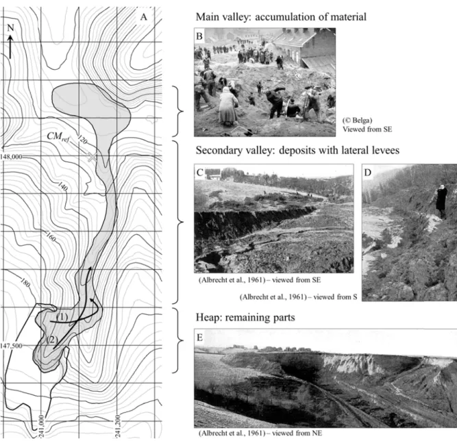
Calembert and Dantinne (1964) give precise topographic maps (scale of 1:1700; contour intervals of 2 m) of the natural topography below the heap, the heap surface before the collapse, and the heap surface after the collapse. Based on these high resolution data, an accurate digital elevation model (DEM) could be created with a kriging method: topographic data are distributed on a 1 × 1 m Cartesian grid (Fig. 1A). Initial material heights were distributed on the same grid (Fig. 1B). A third DEM was created, including the remaining part of the heap as part of the topography instead of the initial material heights (Fig. 1C).
A topographic map covering the entire valley in which the flow occurred is not given by Calembert and Dantinne (1964). Therefore, the DEM used here is based on current topographic data of this narrow and steep-sided valley with a mild-sloped thalweg (~ 3°). A protection embankment built after the collapse has been removed from the model (Fig. 2).
4 <insert Fig. 1 near here>
<insert Fig. 2 near here>
2.3. Collapse and post-failure deposits
The failure of the heap occurred in two phases, as sketched by the arrows in Fig. 2: the initial collapse of the northern part of the heap was followed by a second and more important collapse. The first destabilized mass climbed the opposite slope of the secondary valley before sliding back to the thalweg; the second mass fell in the direction of the thalweg and followed its path. The flow ended in the main valley where it spread out and impacted several houses. The difference between the DEMs in Figs. 1B and 1C indicates that the overall volume of displaced material was about 206,300 m³ (Calembert and Dantinne (1964) gave an estimation of 100,000 to 150,000 m³).
The contour of the deposits was mapped by Calembert and Dantinne (1964) based on aerial photography (Fig. 2). An interesting aerial photograph of the site 11 days after the accident can be found in Bishop (1973, Fig. 25a).
In the secondary valley, the flow left thin deposits, ~ 20 to 30 m wide, bounded by 4-m-high lateral levees (Albrecht et al., 1961). In the main valley, the deposits formed a lens, the thickness of which reached 10 m at its NW end. The lens was delimited by steep slopes, even at the places were the flow had not been stopped by houses. In the houses impacted by the flow, fly ash is reported to have filled each corner, even in the cellars (Calembert and Dantinne, 1964).
The day after the collapse, drillings were made in the deposits in the secondary valley, at a distance of about 100 m from the heap. These drillings showed that there was no mud layer at the base of the deposits. At that time, the deposits in the main valley looked dry. Their water content was found to be equal to that in the upper part of the remaining heap. With a porosity of 0.587, this means a degree of saturation of about 64%. All these observations made by Calembert and Dantinne (1964) in relation with the water content in the deposits contrast with those of Albrecht et al. (1961), who arrived two days later, at a time when the small stream flowing in the secondary valley had made its way through the deposits.
Specific surface measurements on samples from the deposits in the secondary valley revealed a graded bedding, in which larger particles covered finer ones (Calembert and Dantinne, 1964).
2.4. Interpretation
Calembert and Dantinne (1964) ascribed the failure of the fly ash heap to a rising water table caused by heavy rainfalls that occurred at the end of January 1961. They pointed out the contraction of the lower layer of loose ash as it became saturated with water. The porosity values given in Table 2 show that the nonsaturated ash contracts by 25% when it reaches the saturation point. Values from Albrecht et al. (1961) even suggest a contraction of 50%. This contraction implied the creation of cavities in the body of the heap. The upper, nonsaturated part of the heap thus lost its base and fell down. Calembert and Dantinne (1964) highlighted
5
the important volume of air contained in the heap at the time when this falling occurred: in the upper, nonsaturated part, air occupied more than one third of the volume (Table 2). Based on this observation, Calembert and Dantinne (1964) suggested that, as ash particles fell, their permanent contact network was lost and they were left in suspension. These authors therefore compared the flow to a density current and suggested that the ash that reached the main valley was the ash that initially belonged to the upper part of the heap.
3. Discussion on fluidization
3.1. Mobility of the flow
The mobility of a landslide is generally described by the ratio of the fall height HCM of the center of mass to its runout LCM. For the Jupille fly ash flow, these values can be estimated at
HCM = 45 m and LCM = 500 m (Fig. 2). This gives an HCM/LCM ratio of 0.09. In literature, the
HCM/LCM ratio is often approximated by the ratio of the maximum fall height Hmax to the runout distance of the flow Lmax. For the Jupille fly ash flow, the Hmax/Lmax ratio is 0.07.
Several authors have gathered data for different types of landslides and they have evidenced that the Hmax/Lmax ratio decreases when the volume of the displaced material increases. Several regression formulae have been proposed to predict Hmax/Lmax as a function of the volume of the material. Table 3 provides the Hmax/Lmax ratios given by these regression formulae for the 206,300 m³ volume of the Jupille fly ash flow. Only submarine landslides display Hmax/Lmax ratios as low as the 0.09 value observed in Jupille. All other categories of landslides are much less mobile at such low volumes. This confirms the very unique and distinctive behavior of the Jupille fly ash flow.
It has been argued that the runout Lmax instead of the Hmax/Lmax ratio is a function of the volume of the landslide and that Hmax only adds scatter to the data (Legros, 2002). If the runout Lmax is assumed not to depend on the fall height Hmax, then the 700-m runout of the Jupille fly ash flow is no more an outlier (Table 3). However, the formulae used in Table 3 are based on landslides with fall heights generally larger than several hundreds of meters.
<insert Table 3 near here>
3.2. Mean degree of fluidization of the flow
Calembert and Dantinne (1964) rejected the assumption of a water-fluidized flow because they could not find any water-saturated layer at the base of the deposits. A crude calculation of the degree of fluidization of the flow shows that the thickness of such a layer would be substantial, as shown below.
A simple Coulomb slide-block model shows that the HCM/LCM ratio gives an estimate of the apparent friction coefficient at the base of a landslide (Iverson, 2003b):
app tan CM CM H L (1)
6
For the Jupille fly-ash flow, the HCM/LCM ratio of 0.09 corresponds to an apparent friction angle φapp = 5.1°. The physical meaning of this parameter is questionable for large flows, in which spreading, more than sliding, accounts for the runout distance (Staron and Lajeunesse, 2009). The 206,300 m³ volume of displaced material in the case study is however below the threshold of 106 m³, above which spreading effects dominate (Davies, 1982; Iverson, 2003b). Equation (1) neglects the cohesion of the material involved in the landslide. Even if there is a lack of studies on this subject, we assume a breakdown of the apparent cohesion of fly ash by vibrations at the onset of the flow (Calembert and Dantinne, 1964; Geldart, 1973; Iverson, 1997). The very low HCM/LCM ratio supports this assumption.
If a water-fluidization process is postulated, the low value of the apparent friction angle, as compared to the friction angle of the material φ = 20°, would be explained by a reduction in the normal stresses σb caused by basal pore pressures pb:
app app
tan tan tan 1 b tan
b b b b p p (2)
With φapp = 5.1° and φ = 20°, the degree of fluidization pb/σb would be equal to 0.75. If the flow was saturated over a depth hw, the basal pore pressure could be expressed by pb =
αρwghw, in which α would be the ratio of dynamic to hydrostatic pressures. Iverson et al. (2010) observed values of α of about 2 in large-scale water-saturated debris flow experiments. The total stress σb is given by ρgh, with ρ the bulk density and h the flow height (see section 4.2). Thus, a degree of fluidization of 0.75 requires a saturated depth of about 30% of the flow height, which is quite substantial. However, α values higher than 2 could be expected for flows of particles as fine as fly ash.
3.3. Diffusion of air pore pressures
The assumed heap undermining by a rising water table that led huge volumes of ash fall onto an important layer of air is an air-fluidization process that shares similarities with experiments by Roche et al. (2008, 2010) and Roche (2012).
In these experiments, small glass beads were piled up in a horizontal channel closed by a gate, and they were fluidized by a vertical air influx at the base of the reservoir. The gate was then suddenly opened, so as to let the particles flow to the channel, and the air influx was stopped at the same time. The resulting flow was a dense flow with a runout distance twice as long as the runout distance without initial fluidization. Thus, these experiments suggest that the assumption of a density current is not necessary to explain the high mobility of air-fluidized particles.
Records of free surface profiles, particle velocities, and basal pore pressures were made during the air-fluidization experiments. The results showed that initially fluidized particles behave like an inviscid fluid for most of their propagation, which means that energy dissipation is really low (Roche et al., 2008). Pore pressure measurements showed that dynamic pore pressures persist in the flowing mass. In nonfluidized masses, a light self-fluidization phenomenon is even observed (Roche et al., 2010).
7
The air-fluidization results of Roche et al. (2010) can be transposed to Jupille fly ash flow as, according to a classification by Geldart (1973) based on particles size and density, the fly ash particles of diameters in-between 20 and 100 µm belong to the same class (so called ‘group A’) as the glass beads used in the air-fluidization experiments. This class of particles represents ~ 60% of the mass of fly ash involved in the Jupille flow. Fluidization of group A particles is homogenous (no channelization; no bubbles at the minimum fluidization influx). This would not generally be the case for cohesive particles, but Geldart (1973) reported that stirrers can break the effects of cohesion. The agitation induced by the failure of a fly ash heap is likely to have a similar effect on the apparent cohesion of the particles. The air-fluidization experiments are of high relevance for the case study because, as demonstrated hereafter, this process enables us to explain the observations reported by Calembert and Dantinne (1964) by means of a more acceptable mechanism than a density current.
Montserrat et al. (2012) showed that the pore pressure evolution at the base of a static column of initially fluidized particles can be modeled with a one-dimensional vertical diffusion equation and two boundary conditions:
2 2 2 f p p p D D c t z z (3) 0 0 0 z h z p p z (4)In this equation, p is the pore pressure (Pa), t, the time (s), z, the vertical coordinate (m), h, the material height (m), D, the diffusion coefficient (m²/s), γ, the permeability compliance (Pa-1) and cf, the compressibility of air (Pa-1). The diffusion coefficient is defined as
f n f k n c c D (5)where k is the permeability of the material (m²), µ, the viscosity of air (Pa s), nf, the porosity (–), and cn the porosity compressibility (Pa-1).
A dimensional analysis shows that the last term in Eq. (3) can be neglected for thin layers of particles (Montserrat et al., 2012), which is the case in the experiments (heights < 40 cm). Moreover, cn can be neglected when the mixture is not expanded by the fluidization process (which is the case for fluidization rates up to ~ 90%). Montserrat et al. (2012), as well as Roche (2012), computed linear diffusion coefficients by fitting numerical or analytical solutions of Eq. (3) (without the quadratic term) on experimental results. They found values of the order of 10-2 m²/s. These values increased with the height of the initially fluidized column.
<insert Table 4 near here>
In order to verify whether the diffusion coefficients found by Montserrat et al. (2012) and Roche (2012) can be transposed to the Jupille fly ash flow, characteristics of both materials
8
are compared in Table 3. The permeability of fly ash is 22 times lower and its porosity 1.6 times higher than for glass beads. Equation (5) then suggests that the diffusion coefficient of fly ash is 35 times lower than for glass beads. However, an important difference between the case study and the experiments arises from the material heights, which are about 2 orders of magnitude higher in the first case. This means that the pressure necessary to fluidize the material is accordingly higher. This has an impact on the diffusion coefficient through the compressibility of air, cf, which can be approximated as the inverse of the pressure. In the end, the diffusion coefficient expected in the case study is ~ 2–3 times higher than in the air-fluidization experiments.
4. Mathematical and numerical model
4.1. Shallow flow description
The modeling of flows at the earth surface can take advantage of the existence of a main direction of propagation and make use of the so-called ‘shallow flow description’ of mass and momentum conservation. Such an approach is generally considered as state-of-the-art (Iverson, 1997), even if simpler approaches (such as the kinematic wave model) perform surprisingly better in some cases (Ancey et al., 2012).
Like natural landslides and debris flows, fly ash flows are mixtures of several phases (solid particles, water, and air) whose interactions give the flows their distinctive features. They should therefore not be modeled as a single-phase medium with an intrinsic rheology but their modeling should include equations for the evolution of each phase (Iverson, 2003a). This can be achieved either based on the ‘mixture theory’, which uses a simplified equation for the fluid-phase evolution, or with the ‘phase averaged theory’, which writes down mass and momentum equations for each phase (Pitman and Le, 2005). Here, the first approach is followed. The model reproduces the prevailing phenomena governing the flow, i.e., the reduction of the shear resistance by pore pressures and the vertical diffusion of these pressures. No liquid phase is modeled.
The set of equations is made up of mass and momentum conservation of the mixture and basal pore pressure evolution (Iverson and Denlinger, 2001). They are written in a horizontal reference frame:
, , , , 2 2 2 2 0 1 1 x y b x x x y xx b y x xy zz b xz b xy zz b yz b b b b b y y yy x y h u h u h t x y z u h u h u u h h h t x y x y x z u h u u h u h h h t x y y x y p p u p u p D t x y z (6)9
In these equations, the independent variables are the time t (s), the spatial coordinates in the horizontal plane x and y (m), and the vertical coordinate z (m). The primitive unknowns are the flow depth h (m), the flow velocities ux and uy (m/s), and the basal pore pressure p (Pa). The bulk density ρ (kg/m³) and the diffusion coefficient D (m²/s) are constant parameters; zb (m) stands for the topography, which is fixed. The normal stresses σxx and σyy (defined as positive in compression) and the shear stresses τxy, τxz, and τxy must be expressed as functions of the four primitive unknowns so as to close the set of equations. Normal stresses must be seen as total stresses (Iverson, 1997). Variables with a bar are depth-averaged variables; subscripts b denote local variables at the bottom of the flow.
Equation (6) assumes that the mixture is incompressible. Montserrat et al. (2012) observed mixture expansions only for degrees of fluidization higher than ~ 90%.
The flow velocities are supposed to be uniform over the flow depth. This is correct at the fronts of air-fluidized flows, where the flow is plug-like, but not in their bodies, where pronounced velocity gradients and a static basal layer are observed (Girolami et al., 2010).
4.2. Stresses and stress gradients
Expressions of the stresses in Eq. (6) classically take advantage of the z-momentum equation and the shallowness of the flow, which underline the ‘hydrostatic’ distribution of the mean stress within the flow (Savage and Hutter, 1989). A dimensional analysis of the x- and y-momentum equations also shows that the basal stresses σzz,b, τxz,b, and τyz,b prevail over the internal stress gradients; the normal stress gradients should, however, be kept for a proper modeling of nonuniform flows (Savage and Hutter, 1989). Therefore, we assume
, 0 0 2 zz b xx yy xy xy gh h h gh x y (7)In dense granular flows, basal shear stresses are proportional to the normal stress (GDR MiDi, 2004; Forterre and Pouliquen, 2008). This proportionality holds when an interstitial fluid is present, provided that the pore pressure p is subtracted from the total normal stress (Cassar et al., 2005). The friction coefficient increases with the shear rate experienced by the flow, but this dependence is negligible in the case study owing to important flow depths and small particle sizes; the friction coefficient is thus taken as the tangent of the static friction angle φ. The shear stress is assumed to be aligned with the depth-averaged flow velocity:
, 2 2 , 2 2 tan tan x xz b b x y y yz b b x y u gh p u u u gh p u u (8)4.3. Pore pressures evolution
The pore pressure evolution equation in (6) is a local continuity equation in which two processes are considered (Iverson and Denlinger, 2001):
10 diffusion, occurring in the z direction; and
passive convection, prevailing over diffusion in the x and y directions.
A derivation of the diffusive term for the case of air can be found in Montserrat et al. (2012). The quadratic term from Eq. (3) can be dropped because of the impermeability condition (4). The evaluation of the diffusive term would normally require a computation of the whole pressure field over the flow depth (e.g., Iverson and Denlinger, 2001; Roche, 2012). To avoid the difficulties linked with such a computation (definition of an initial distribution), we approximated the second spatial derivative by the best finite difference expression consistent with the boundary conditions (4). The pore pressure evolution equation then reads (Iverson et al., 2010) x
2 2 b b b y b p D p u p u p t x y h (9)The diffusion term in Eq. (9) displays a very interesting behavior: pore pressures are dissipated more rapidly in areas where the flow depth h is low, i.e., at the margins of the flow. This feature is shared by other formulations of the vertical diffusion model (Iverson and Denlinger, 2001). Such a model induces a spatial distribution of the resistance to flow, which has been identified by many authors as a fundamental feature of water- or air-fluidized granular flows (Iverson, 2005; Ancey, 2007; Girolami et al., 2010) and appears to be of importance for the Jupille fly ash flow (lateral levees, steep flow front). Even nonfluidized granular flows display such a behavior, because of the dependence of the friction coefficient on the shear rate (Félix and Thomas, 2004; Mangeney et al., 2007). However, as this dependence has been identified as negligible in the present case study, pore pressure effects are thought to prevail.
4.4. Numerical model
Numerical modelling of the flow was performed with an adapted version of the academic hydraulic model WOLF 2D, developed at the University of Liege. A detailed description of the initial model was provided by Dewals et al. (2008) and Erpicum et al. (2010b).
The model solves Eq. (6) using a Cartesian grid and a second-order accurate finite volume scheme. The fluxes are computed by a self-developed flux vector splitting, which is Froude-independent and well-balanced with respect to the pressure and bottom slope terms (Erpicum et al., 2010b). The time integration is performed by means of a three-step Runge-Kutta algorithm, and a semi-implicit treatment of the bottom friction term is used. The time step is adaptive and computed based on the Courant-Friedrichs-Lewy (CFL) stability criterion, with a CFL number equal to 0.5. It takes values of the order of 10-3 – 10-2 s.
This finite volume model has already proven its validity and efficiency for the analysis of natural and artificial floods (Ernst et al., 2010; Erpicum et al., 2010a; Dewals et al., 2011), as well as numerous other applications including complex turbulent flows (Dewals et al., 2008; Erpicum et al., 2009; Roger et al., 2009; Dufresne et al., 2011).
11
5. Results
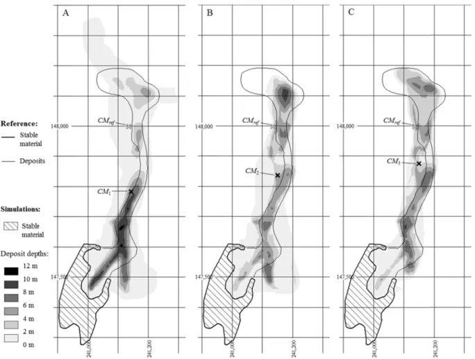
The numerical results are presented in three steps so as to highlight the influence of pore pressure generation and dissipation (Table 5). In step 1, instantaneous fluidization is assumed and no diffusion phenomenon is considered: the degree of fluidization is uniform and remains constant during the flow. In step 2, the diffusion of pore pressures is taken into account: this induces a progressive decrease in the degree of fluidization that becomes nonuniform during the propagation of the flow. In step 3, progressive fluidization is considered: the failure-triggering degree of fluidization is not reached in the whole heap at the same time.
The assessment of the accuracy of the results is based on two features of the final deposits: the area they cover and their morphology. The runout area is compared to the reference displayed in Fig. 2. The deposit depths could be compared to the approximate values given in section 2.3, but a comparison based on the location of the center of mass gives a more synthetic overview of the depth distribution. The reference location of the center of mass displayed in Fig. 2 is obtained by assuming a mean deposit depth of 3 m in the secondary valley and a mean deposit depth of 7 m in the main valley. This simple assumption is consistent with the volume of displaced material given in section 2.3.
<insert Table 5 near here>
5.1. Results with a uniform and constant degree of fluidization
In a first step, the whole mass of the material situated above the failure surface displayed in Fig. 1C is assumed to be instantaneously fluidized and no pore pressure dissipation is taken into account during the subsequent flow. A degree of fluidization of 75% is postulated (Table 5) in accordance with section 3.2. Results are displayed in Fig. 3A and 4. The runout distance is largely overestimated. However, the distance travelled by the center of mass is underestimated by more than 200 m because most of the material stops in the secondary valley and does not reach the main valley. These results are in contradiction with the observations reported in section 2.3. They underline that the mobility of the actual flow cannot be reached with a model that neglects pore pressure dissipation.
5.2. Influence of pore pressure dissipation
In a second step, vertical diffusion is included in the simulations. Fig. 3 displays the results obtained starting with a completely fluidized material (Table 5). The diffusion coefficient
D = 0.25 m²/s is taken one order of magnitude higher than the diffusion coefficients in
small-scale laboratory tests, but it remains an acceptable value given the complex pore pressure dissipation mechanisms that take place in such a large-scale flow. The simulation highlights that despite the high diffusion coefficient (with water in place of air, the diffusion coefficient would be ~ 1000 times lower), the diffusion phenomenon is still sufficiently slow for pore pressures to be kept high enough during a flow of hundreds of meters.
Results are displayed in Fig. 3B and 4. Even if the runout distance is now underestimated, the final center of mass lies closer to its estimated reference location than in step 1. The ratio of the distance travelled by the center of mass to the distance travelled by the flow front is thus increased. An important part of the fly ash mass now reaches the larger valley. The
12
longitudinal section displayed in Fig. 4 shows that this mass has a steep front. This is induced by the spatial distribution of the resistance to flow induced by the diffusion model (section 4.3) and is in accordance with observations. The result of step 2 shares another similarity with the observed deposit’s morphology: the presence of lateral levees (Fig. 3B).
<insert Fig. 3 near here> <insert Fig. 4 near here>
An important difference between numerical results and observations is the runout area in the vicinity of the heap. The assumption of an instantaneous fluidization leads to an initially widespread flow as compared to the relatively concentrated flow observed in reality. There is thus a waste of momentum in this region because, in the simulations, an important mass rushes in a wrong direction before being redirected by the topography of the valley. Step 3, in which the collapse is progressive, improves this aspect.
5.3. Influence of pore pressure generation
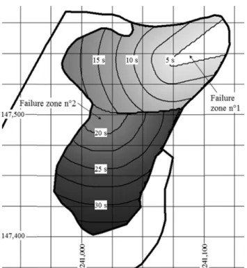
In a last step, the progressive nature of the failure is taken into account. For this purpose, a distinction is made between a nonfluidized and a fluidized state. In the first state, no pore pressures are taken into account in the basal friction terms and a specific cohesion of c/ρ = 200 m²/s² is added to Eq. (8) so that the entire heap is stable. In the fluidized state, pore pressures are initiated and the cohesion of the material disappears. The time at which the initially stable material becomes fluidized is prescribed a priori, as shown in Fig. 5. The spatial distribution used for the time of failure enables us to reproduce the two phases of the failure, as shown in Fig. 2. Note that in a risk analysis, the time of failure is not known, but the method followed here can be replaced by a method based on a dynamic threshold to account for a progressive failure.
<insert Fig. 5 near here> <insert Fig. 6 near here>
Results are displayed in Figs. 3C and 4. The objective of a more concentrated flow in the initial phase is reached. This has an impact on the overall runout distance and on the amount of fly ash that piles up in the main valley. Even if the flow duration is longer with a progressive collapse (78 s instead of 57 s in step 2), the vertical diffusion process is still low enough to ensure a sufficient degree of fluidization during propagation. This is shown in Fig. 6, which compares the degree of fluidization after 60 s for steps 1 to 3. This figure also shows the preferential decrease of pore pressure at the margins of the flow, as explained in section 4.3.
6. Conclusion
The fly ash heap collapse that occurred in Jupille in 1961 developed into a highly fluidized flow. Based on field evidence, Calembert and Dantinne (1964) suggested that, instead of water, interstitial air played a key role in the fluidization process. Air-fluidization theories proposed in the 1960s and 1970s have since been rejected in the field of landslide modeling
13
and air is generally considered to play only a secondary role (Legros, 2002). However, in the Jupille case study, the identified failure mechanism and the properties of the material support the assumption of an air-fluidized flow. The initial collapse phase was a downfall of the upper, nonsaturated layer of the heap onto its undermined base, followed by a diffusion of the resulting pore pressures through the mass of fly ash. In this paper, this assumed failure mechanism was tested using a 2D numerical model focusing on the most prominent processes governing the flow. The aim was to verify whether an air-fluidization theory was consistent with field observations.
Based on the analysis of observed data, we first underlined the high degree of fluidization of the flow. Then, assuming that the high degree of fluidization resulted from the compression of the interstitial air, numerical results have shown that, even if a high diffusion coefficient is used, an important degree of fluidization can be maintained inside the flow during most of its propagation. Progressive enhancements of the model as regards pore pressure generation and dissipation showed that these phenomena are critical to reproduce the field observations: they increased the mobility of the computed flow and led to deposits displaying the same morphological characteristics observed in reality (steep front, lateral levees). Although further enhancements are needed to accurately reproduce the lateral spreading in the secondary valley, these results confirm the overall agreement between field data and numerical predictions based on the assumption of air fluidization. Further developments can take advantage of the description of the available data of the Jupille fly ash flow presented in this paper.
References
Albrecht, K., Brühl, H., Langguth, H.R., 1961. Eine Kippenrutschung in Moulins-sous-Fléron bei Lüttich. Geologische Mitteilungen 2(1), 38-48.
Ancey, C., 2007. Plasticity and geophysical flows: a review. Journal of Non-Newtonian Fluid Mechanics 142, 4-35.
Ancey, C., Andreini, N., Epely-Chauvin, G., 2012. Viscoplastic dambreak waves: review of simple computational approaches and comparison with experiments. Advances in Water Resources 48, 79-91.
Bishop, A.W., 1973. The stability of tips and spoil heaps. Quarterly Journal of Engineering Geology and Hydrogeology 6, 335-376.
Calembert, L., Dantinne, R., 1964. L'avalanche de cendres volantes survenue à Jupille (Liège) le 3 février 1961. In: Spronck, R. (Ed.), Amici et Alumni - Hommage à Ferdinand Campus. Georges Thone, Liège, Belgium, pp. 41-57.
Cassar, C., Nicolas, M., Pouliquen, O., 2005. Submarine granular flows down inclined planes. Physics of Fluids 17, 103301.
Corominas, J., 1996. The angle of reach as a mobility index for small and large landslides. Canadian Geotechnical Journal 33, 260-271.
Davies, T.R.H., 1982. Spreading of rock avalanche debris by mechanical fluidization. Rock Mechanics 15, 9-24.
14
Dewals, B., Kantoush, S., Erpicum, S., Pirotton, M., Schleiss, A.J., 2008. Experimental and numerical analysis of flow instabilities in rectangular shallow basins. Environmental Fluid Mechanics 8, 31-54.
Dewals, B., Erpicum, S., Detrembleur, S., Archambeau, P., Pirotton, M., 2011. Failure of dams arranged in series or in complex. Natural Hazards 56(3), 917-939.
Dufresne, M., Dewals, B., Erpicum, S., Archambeau, P., Pirotton, M., 2011. Numerical investigation of flow patterns in rectangular shallow reservoirs. Engineering Applications of Computational Fluid Mechanics 5(2), 247-258.
Ernst, J., Dewals, B., Detrembleur, S., Archambeau, P., Erpicum, S., Pirotton, M., 2010. Micro-scale flood risk analysis based on detailed 2D hydraulic modelling and high resolution geographic data. Natural Hazards 55(2), 181-209.
Erpicum, S., Meile, T., Dewals, B., Pirotton, M., Schleiss, A.J., 2009. 2D numerical flow modeling in a macro-rough channel. International Journal for Numerical Methods in Fluids 61(11), 1227-1246.
Erpicum, S., Dewals, B., Archambeau, P., Detrembleur, S., Pirotton, M., 2010a. Detailed inundation modelling using high resolution DEMs. Engineering Applications of Computational Fluid Mechanics 4(2), 196-208.
Erpicum, S., Dewals, B., Archambeau, P., Pirotton, M., 2010b. Dam-break flow computation based on an efficient flux-vector splitting. Journal of Computational and Applied Mathematics 234(7), 2143-2151.
Félix, G., Thomas, N., 2004. Relation between dry granular flow regimes and morphology of deposits: formation of levées in pyroclastic deposits. Earth and Planetary Science Letters 221, 197-213.
Forterre, Y., Pouliquen, O., 2008. Flows of dense granular media. Annual Reviews of Fluid Mechanics 40, 1-24.
GDR MiDi, 2004. On dense granular flows. The European Physical Journal E 14, 341-365. Geldart, D., 1973. Types of gas fluidization. Powder Technology 7, 285-292.
Girolami, L., Roche, O., Druitt, T.H., Corpetti, T., 2010. Particle velocity fields and depositional processes in laboratory ash flows, with implications for the sedimentation of dense pyroclastic flows. Bulletin of Volcanology 72, 747-759.
Hayashi, J.N., Self, S., 1992. A comparison of pyroclastic flow and debris avalanche mobility. Journal of Geophysical Research 97, 9063-9071.
Hsü, K.J., 1975. Catastrophic debris streams (sturzstroms) generated by rockfalls. Geological Society of America Bulletin 86(1), 129-140.
Iverson, R.M., 1997. The physics of debris flows. Reviews of Geophysics 35(3), 245-296. Iverson, R.M., 2003a. The debris-flow rheology myth. In: Rickenmann, D., Chen, C.L.
(Eds.), Debris-flow Hazards Mitigation: Mechanics, Prediction, and Assessment. Millpress, Roterdam, The Netherlands, pp. 303-314.
Iverson, R.M., 2003b. How should mathematical models of geomorphic processes be judged? In: Wilcock, P.R., Iverson, R.M. (Eds.), Prediction in Geomorphology. Geophysical Monograph Series. AGU, Washington, DC, pp. 83-94.
Iverson, R.M., 2005. Debris-flow mechanics. In: Jakob, M., Hungr, O. (Eds.), Debris-flow Hazards and Related Phenomena. Praxis, Springer, Berlin, Heidelberg, pp. 105-134.
15
Iverson, R.M., Denlinger, R.P., 2001. Flow of variably fluidized granular masses across three-dimensional terrain - 1. Coulomb mixture theory. Journal of Geophysical Research 106, 537-552.
Iverson, R.M., Logan, M., LaHusen, R.G., Berti, M., 2010. The perfect debris flow? Aggregated results from 28 large-scale experiments. Journal of Geophysical Research 115, F03005.
Legros, F., 2002. The mobility of long-runout landslides. Engineering Geology 63, 301-331. Mangeney, A., Bouchut, F., Thomas, N., Vilotte, J.P., Bristeau, O., 2007. Numerical
modelling of self-channeling granular flows and their levee-channel deposits. Journal of Geophysical Research 112, F02017.
Montserrat, S., Tamburrino, A., Roche, O., Niño, Y., 2012. Pore fluid pressure diffusion in defluidizing granular columns. Journal of Geophysical Research 117, F02034.
Pitman, E.B., Le, L., 2005. A two-fluid model for avalanche and debris flows. Philosophical Transactions of the Royal Society A 363, 1573-1601.
Roche, O., 2012. Depositional processes and gas pore pressure in pyroclastic flows: an experimental perspective. Bulletin of Volcanology 74, 1807-1820.
Roche, O., Montserrat, S., Niño, Y., Tamburrino, A., 2008. Experimental observations of water-like behavior of initially fluidized, dam break granular flows and their relevance for the propagation of ash-rich pyroclastic flows. Journal of Geophysical Research 113, B12203.
Roche, O., Montserrat, S., Niño, Y., Tamburrino, A., 2010. Pore fluid pressure and internal kinematics of gravitational laboratory air-particle flows: insights into the emplacement dynamics of pyroclastic flows. Journal of Geophysical Research 115, B09206.
Roger, S., Dewals, B., Erpicum, S., Schwanenberg, D., Schüttrumpf, H., Köngeter, J., Pirotton, M., 2009. Experimental and numerical investigations of dike-break induced flows. Journal of Hydraulic Research 47(3), 349-359.
Savage, S.B., Hutter, K., 1989. The motion of a finite mass of granular material down a rough incline. Journal of Fluid Mechanics 199, 177-215.
Staron, L., Lajeunesse, E., 2009. Understanding how volume affects the mobility of dry debris flows. Geophysical Research Letters 36, L12402.
Figure
Fig. 1. failure s (1964). × 50 m)es
(A) Topog surface inter Contour in ); bold lines graphy befo rpolated on ntervals are s show the li re heap con a 1 × 1 m C 5 m; refere imit of the h 16 nstruction, Cartesian gr ence grid is heap and th (B) fly ash rid from ma in 1972 Be he failure su h heap befo aps by Calem elgian Lamb rface. ore failure, mbert and D bert coordin and (C) Dantinne nates (50Fig. 2. ( area cov initial fl 100 m deposits (A) Topogr vered by th flow directio reference g s. raphy interp he fly ash f ons (arrows grid in 19 polated on a flow accord s), and estim 72 Belgian 17 a 1 × 1 m C ding to Cale mated final n Lambert Cartesian gri embert and location of coordinate id (contour Dantinne ( f center of m s. (B-E) P intervals of (1964) (fille mass (CMref Photographs f 2.5 m), ed area), f); 100 × s of the
Fig. 3. D uniform account Fig. 4. valley. Deposit dep m and consta t; (C) step 3 Longitudin pths and ce ant degree o – pore pres nal section o nter of mas of fluidizati ssure genera of final dep 18 ss locations ion; (B) ste ation and di posits along s (CM) for t ep 2 – pore issipation ta g the thalwe three simula pressure dis aken into ac eg of the se ations: (A) ssipation ta ccount. econdary a step 1 – aken into and main
Fig. 5. T Fig. 6. D and for – pore dissipat Time at whi Degree of fl three simul pressure di tion taken in
ich the mate
luidization i lations: (A) issipation t nto account. erial becom in the flow, step 1 – un aken into a . 19 mes fluidized , 60 s after t niform and account; (C d in the step the initial fa constant de C) step 3 – p 3 numerica ailure, for fl egree of flui pore press al simulatio low depths idization; (B sure generat on. > 10-4 m B) step 2 tion and
20
Tables
Table 1
Fly ash grading. Percentages are on a mass basis. Measurements were performed on four probes taken from the remaining part of the heap at depths varying between 0.6 and 2.3 m. Minimum and maximum values are obtained from the deepest and shallowest probes, respectively. Data source: Calembert and Dantinne (1964).
d10 d20 d50 d60 d80 d90
Mean value (µm) 11 18 35 45 106 420
Range of values (µm) 10-12 17-20 32-40 39-54 63-181 93-1211
Table 2
Representative densities and volumetric properties of the fly ash of the heap. Data source: CD: Calembert and Dantinne (1964); ABL: Albrecht et al. (1961).
Ref. Bulk density Porosity Degree of saturation Upper, nonsaturated part
CD ABL 1020 kg/m³ 1000 kg/m³ 0.67 0.71 45.3% 56.3% Lower, water-saturated part
CD ABL 1510 kg/m³ 1600 kg/m³ 0.55 0.41 100% 100%
21 Table 3
Hmax/Lmax ratio and runout for different categories of landslides having a volume of 206,300 m³, as computed by regression formulae given by different authors.
Authors Landslide category Ratio Hmax/Lmax Runout Lmax Hayashi and Self (1992) Volcanic debris avalanches 0.23
Nonvolcanic debris avalanches 0.59
Pyroclastic flows 0.30
Corominas (1996) Rockfalls 0.43
Debris flows 0.27
Earth flows and mudslides 0.26
Translational slides 0.30
Legros (2002) Nonvolcanic landslides 0.57 960 m
Volcanic landslides 0.55 570 m
Martian landslides 2.11 350 m
Submarine landslides 0.06 1090 m
Debris flows / 8590 m
Table 4
Comparison between characteristics of the material used in air-fluidization experiments (Roche, 2012) and the material involved in the Jupille case study (Calembert and Dantinne, 1964).
Material Particle
size
Solid phase density
Porosity Permeability Material height
µm kg/m³ m² m
Experiments Glass beads 60 – 90 2500 0.4 1.1 × 10⁻¹¹ 0.05 – 0.35 Case study Fly ash 40 2150 0.667 5 × 10-13 5 – 30
22 Table 5
Assumptions and parameters used for numerical simulations.
Step 1 Step 2 Step 3
Pore pressure generation Instantaneous Instantaneous Progressive Pore pressure dissipation None Vertical diffusion Vertical diffusion
Friction angle 20° 20° 20°
Initial degree of fluidization 0.75 1.00 1.00
Diffusion coefficient None 0.25 m²/s 0.25 m²/s