The TRAPPIST survey of southern transiting planets. I. Thirty eclipses of the ultra-short period planet WASP-43 b

(1)

arXiv:1201.2789v2 [astro-ph.EP] 31 May 2012

Astronomy & Astrophysicsmanuscript no. WASP-43 _{ESO 2012}c

June 1, 2012

The TRAPPIST survey of southern transiting planets. I

Thirty eclipses of the ultra-short period planet WASP-43 b

⋆

M. Gillon

1

, A. H. M. J. Triaud

2

, J. J. Fortney

3

, B.-O. Demory

4

, E. Jehin

1

, M. Lendl

2

, P. Magain

1

, P. Kabath

5

,

D. Queloz

2

, R. Alonso

2

, D. R. Anderson

6

, A. Collier Cameron

7

, A. Fumel

1

, L. Hebb

8

, C. Hellier

6

, A. Lanotte

1

,

P. F. L. Maxted

6

, N. Mowlavi

2

, B. Smalley

6 1_{Université de Liège, Allée du 6 août 17, Sart Tilman, Liège 1, Belgium}

2_{Observatoire de Genève, Université de Genève, 51 Chemin des Maillettes, 1290 Sauverny, Switzerland} 3_{Department of Astronomy and Astrophysics, University of California, Santa Cruz, CA 95064, USA}

4 _{Department of Earth, Atmospheric and Planetary Sciences, Department of Physics, Massachusetts Institute of Technology, 77} Massachusetts Ave., Cambridge, MA 02139, USA

5_{European Southern Observatory, Alonso de Cordova 3107, Casilla 19001, Santiago, Chile} 6_{Astrophysics Group, Keele University, Staffordshire ST5 5BG, UK}

7_{School of Physics and Astronomy, University of St. Andrews, North Haugh, Fife, KY16 9SS, UK} 8_{Department of Physics and Astronomy, Vanderbilt University, Nashville, TN 37235, USA}

Received date / accepted date

ABSTRACT

We present twenty-three transit light curves and seven occultation light curves for the ultra-short period planet WASP-43 b, in addition to eight new measurements of the radial velocity of the star. Thanks to this extensive data set, we improve significantly the parameters of the system. Notably, the largely improved precision on the stellar density (2.41 ± 0.08 ρ⊙) combined with constraining the age to be

younger than a Hubble time allows us to break the degeneracy of the stellar solution mentioned in the discovery paper. The resulting stellar mass and size are 0.717 ± 0.025 M⊙and 0.667 ± 0.011 R⊙. Our deduced physical parameters for the planet are 2.034 ± 0.052

MJupand 1.036 ± 0.019 RJup. Taking into account its level of irradiation, the high density of the planet favors an old age and a massive

core. Our deduced orbital eccentricity, 0.0035+0.0060

−0.0025, is consistent with a fully circularized orbit. We detect the emission of the planet

at 2.09 µm at better than 11-σ, the deduced occultation depth being 1560 ± 140 ppm. Our detection of the occultation at 1.19 µm is marginal (790 ± 320 ppm) and more observations are needed to confirm it. We place a 3-σ upper limit of 850 ppm on the depth of the occultation at ∼0.9 µm. Together, these results strongly favor a poor redistribution of the heat to the night-side of the planet, and marginally favor a model with no day-side temperature inversion.

Key words.stars: planetary systems - star: individual: WASP-43 - techniques: photometric - techniques: radial velocities

1. Introduction

There are now more than seven hundreds planets known to or-bit around other stars than our Sun (Schneider 2011). A signifi-cant fraction of them are Jovian-type planets orbiting within 0.1 AU of their host stars. Their very existence poses an interest-ing challenge for our theories of planetary formation and evo-lution, as such massive planets could not have formed so close to their star (D’Angelo et al. 2010; Lubow & Ida 2010). Long neglected in favor of disk-driven migration theories (Lin et al. 1996), the postulate that past dynamical interactions combined with tidal dissipation could have shaped their present orbit has raised a lot of interest recently (e.g. Fabrycky & Tremaine 2007, Naoz et al. 2011, Wu & Lithwick 2011), partially thanks to the discovery that a significant fraction of these planets have high orbital obliquities that suggest past violent dynamical perturba-tions (e.g. Triaud et al. 2010).

Send offprint requests to: michael.gillon@ulg.ac.be

⋆ _{Based on data collected with the TRAPPIST and Euler telescopes}

at ESO La Silla Observatory, Chile, and with the VLT/HAWK-I instru-ment at ESO Paranal Observatory, Chile (program 086.C-0222).

Not only the origin of these planets but also their fate raises many questions. Their relatively large mass and small semi-major axis imply tidal interactions with the host star that should lead in most cases to a slow spiral-in of the planet and to a trans-fer of angular momentum to the star (e.g. Barker & Ogilvie 2009, Jackson et al. 2009, Mastumura et al. 2010), the end result be-ing the planet’s disruption at its Roche limit (Gu et al. 2003). The timescale of this final disruption depends mostly on the timescale of the migration mechanism, the tidal dissipation ef-ficiency of both bodies, and the efef-ficiency of angular momentum losses from the system due to magnetic braking. These three pa-rameters being poorly known, it is desirable to detect and study in depth ‘extreme’ hot Jupiters, i.e. massive planets having ex-ceptionally short semi-major axes that could be in the final stages of their tidal orbital decay.

The WASP transit survey detected two extreme examples of such ultra-short period planets, WASP-18 b (Hellier et al. 2009) and WASP-19 b (Hebb et al. 2010), both having an orbital period smaller than one day. Thanks to their transiting nature, these sys-tems were amenable for a thorough characterization that made possible a study of the effects of their tidal interactions (Brown et al. 2011). Notably, photometric observations of some of their

(2)

occultations made possible not only to probe both planets’ day-side emission spectra but also to bring strong constraints on their orbital eccentricity (Anderson et al. 2010, Gibson et al. 2010, Nymeyer et al. 2011), a key parameter to assess their tidal his-tory and energy budget. The same WASP survey has recently an-nounced the discovery of a third ultra-short period Jovian planet called WASP-43 b (Hellier et al. 2011b, hereafter H11). Its or-bital period is 0.81 d, the only hot Jupiter having a smaller pe-riod being WASP-19 b (0.79 d). Furthermore, it orbits around a very cool K7-type dwarf that has the lowest mass among all the stars orbited by a hot Jupiter (0.58 ± 0.05M⊙, Te f f = 4400 ± 200 K, H11), except for the recently announced M0 dwarf KOI-254 (0.59 ± 0.06M⊙, Te f f = 3820 ± 90 K, Johnson et al. 2011).

Nevertheless, H11 presented another plausible solution for the stellar mass that is significantly larger, 0.71 ± 0.05M⊙. This

de-generacy translates into a poor knowledge of the physical pa-rameters of the system.

With the aim to improve the characterization of this interest-ing ultra-short period planet, we performed an intense ground-based photometric monitoring of its eclipses (transits and occul-tations), complemented with new measurements of the radial ve-locity (RV) of the star. These observations were carried out in the frame of a new photometric survey based on the 60cm robotic telescope TRAPPIST1 _{(TRAnsiting Planets and PlanetesImals}

Small Telescope; Gillon et al. 2011a, Jehin et al. 2011). The

concept of this survey is the intense high-precision photomet-ric monitoring of the transits of southern transiting systems, its goals being (i) to improve the determination of the physical and orbital parameters of the systems, (ii) to assess the presence of undetected objects in these systems through variability studies of the transit parameters, and (iii) to measure or put an upper limit on the very-near-IR thermal emission of the most highly irradiated planets to constrain their atmospheric properties. We complemented the data acquired in the frame of this program for the WASP-43 system by high-precision occultation time-series photometry gathered in the near-IR with the VLT/HAWK-I in-strument (Pirard et al., 2004, Casali et al. 2006) in our program 086.C-0222. We present here the results of the analysis of this extensive data set. Section 2 below presents our data. Their anal-ysis is described in Sec. 3. We discuss the acquired results and drawn inferences about the WASP-43 system in Sec. 4. Finally, we give our conclusions in Sec. 5.

2. Data

2.1. TRAPPISTI+zfilter transit photometry

We observed 20 transits of WASP-43 b with TRAPPIST and its thermoelectrically-cooled 2k × 2k CCD camera with a field of view of 22’ × 22’ (pixel scale = 0.65”). All the 20 transits were observed in an Astrodon ‘I+z’ filter that has a transmittance >90% from 750 nm to beyond 1100 nm2, the red end of the effec-tive bandpass being defined by the spectral response of the CCD. This wide red filter minimizes the effects of limb-darkening and differential atmospheric extinction while maximizing stel-lar counts. Its effective wavelength for Te f f = 4400 ± 200 K is λe f f _{= 843.5 ± 1.2 nm. The mean exposure time was 20s.} The telescope was slightly defocused to minimize pixel-to-pixel effects and to optimize the observational efficiency. We gener-ally keep the positions of the stars on the chip within a box of a few pixels of side to improve the photometric precision of our

1 _{see http://www.ati.ulg.ac.be/TRAPPIST}

2 _{see http://www.astrodon.com/products/filters/near-infrared/}

TRAPPIST time-series, thanks to a ‘software guiding’ system deriving regularly astrometric solutions on the science images and sending pointing corrections to the mount if needed. It could unfortunately not be used for WASP-43, because the star lies in a sky area that is not covered by the used astrometric catalogue (GSC1.1). This translated into slow drifts of the stars on the chip, the underlying cause being the imperfection of the telescope po-lar alignment. The amplitudes of those drifts on the total duration of the runs were ranging between 15 and 85 pixels in the right ascension direction and between 5 and 75 pixels in the declina-tion direcdeclina-tion. Table 1 presents the logs of the observadeclina-tions. The first of these 20 transits was presented in H11.

After a standard pre-reduction (bias, dark, flatfield correc-tion), the stellar fluxes were extracted from the images using the IRAF/DAOPHOT3aperture photometry software (Stetson, 1987). For each transit, several sets of reduction parameters were tested, and we kept the one giving the most precise photometry for the stars of similar brightness as WASP-43. After a careful selection of reference stars, differential photometry was then obtained. The resulting light curves are shown in Fig. 1 and 2.

2.2.EulerGunn-r′_{filter transit photometry}

Three transits of WASP-43 b were observed in the Gunn-r′

fil-ter (λe f f _{= 620.4 ± 0.5 nm) with the EulerCAM CCD camera} at the 1.2-m Euler Swiss telescope, also located at ESO La Silla Observatory. EulerCAM is a nitrogen-cooled 4k × 4k CCD cam-era with a 15’ × 15’ field of view (pixel scale=0.23”). Here too, the telescope was slightly defocused to optimize the photometric precision. The mean exposure time was 85s. The stars were kept approximately on the same pixels, thanks to a ‘software guiding’ system similar to TRAPPIST’s but using the UCAC3 catalogue. The calibration and photometric reduction procedures were sim-ilar to the ones performed on the TRAPPIST data. The logs of these Euler observations are shown in Table 1, while the result-ing light curves are visible in Fig. 2. Notice that the first of these

Euler transits was presented in H11.

2.3. TRAPPISTz′_{filter occcultation photometry}

Five occultations of WASP-43 b were observed with TRAPPIST in a Sloan z’ filter (λe f f _{= 915.9 ± 0.5 nm). Their logs are} pre-sented in Table 1. The mean exposure time was 40s. The cali-bration and photometric reduction of these occultation data were similar to the ones of the transits. Fig. 3 shows the resulting light curves with their best-fit models.

2.4. VLT/HAWK-I 1.19 and 2.09µm occultation photometry

We observed two occultations of WASP-43 b with the cryogenic near-IR imager HAWK-I at the ESO Very Large Telescope in our program 086.C-0222. HAWK-I is composed of four Hawaii 2RG 2048× 2048 pixels detectors (pixel scale = 0.106”), its to-tal field of view on the sky being 7.5’×7.5’. We choose to ob-serve the occultations within the narrow band filters NB2090 (λ = 2.095 µm, width = 0.020 µm) and NB1190 (λ = 1.186 µm, width = 0.020 µm), respectively. The small width of these cosmological filters minimizes the effect of differential extinc-tion. Furthermore, they avoid the largest absorption and

emis-3 _IRAF _is _distributed _by _the _National _Optical _Astronomy Observatory, which is operated by the Association of Universities for Research in Astronomy, Inc., under cooperative agreement with the National Science Foundation.

(3)

Date Instrument Filter Np Epoch Baseline σ σ120s βw βr CF

function [%] [%]

06 Dec 2010 TRAPPIST I+z 393 11 p(t2₎ _{0.35, 0.36} _{0.14, 0.17} _{1.26, 1.30} _{1.00, 1.90} _{1.26, 2.47}

09 Dec 2010 VLT/HAWK-I NB2090 183 13.5 p(t2_{) + p(l}1_{) + p(xy}1₎ _{0.055, 0.055} _{0.036, 0.036} _{1.04, 1.04} _{1.09, 1.14} _{1.14, 1.18}

28 Dec 2010 Euler Gunn-r′ 111 38 p(t2_{) + p(xy}2₎ _{0.10, 0.10} _{0.10, 0.10} _{1.54, 1.64} _{1.04, 1.15} _{1.61, 1.90}

30 Dec 2010 TRAPPIST z′ ₃₃₂ _40.5 _p(t2₎ _{0.30, 0.30} _{0.14, 0.14} _{1.04, 1.04} _{1.00, 1.00} _{1.04, 1.04}

01 Jan 2011 TRAPPIST I+z 407 43 p(t2_{) + p(xy}2₎ _{0.27, 0.27} _{0.11, 0.12} _{1.00, 1.01} _{1.00, 1.00} _{1.00, 1.01}

06 Jan 2011 TRAPPIST I+z 273 49 p(t2₎ _{0.24, 0.24} _{0.11, 0.11} _{1.07, 1.09} _{1.00, 1.38} _{1.07, 1.50}

09 Jan 2011 VLT/HAWK-I NB1190 115 51.5 p(t2_{) + p(b}1_{) + p(xy}1₎ _{0.087, 0.087} _{0.047, 0.048} _{2.22, 2.22} _{1.00, 1.00} _{2.22, 2.22}

23 Jan 2011 TRAPPIST I+z 244 70 p(t2_{) + p(xy}2₎ _{0.20, 0.20} _{0.08, 0.09} _{1.02, 1.02} _{1.00, 1.00} _{1.02, 1.02}

28 Jan 2011 Euler Gunn-r′ 114 76 p(t2_{) + p(xy}1₎ _{0.13, 0.13} _{0.13, 0.13} _{1.36, 1.42} _{1.17, 1.24} _{1.59, 1.76}

06 Feb 2011 Euler Gunn-r′ ₁₀₇ ₈₇ _p(t2₎ _{0.13, 0.15} _{0.13, 0.15} _{0.92, 1.07} _{1.10, 1.86} _{1.02, 1.99}

14 Feb 2011 TRAPPIST I+z 311 97 p(t2₎ _{0.21, 0.22} _{0.11, 0.12} _{1.05, 1.08} _{1.00, 1.42} _{1.05, 1.53}

08 Mar 2011 TRAPPIST I+z 285 124 p(t2₎ _{0.21, 0.22} _{0.11, 0.13} _{1.11, 1.15} _{1.00, 2.00} _{1.11, 2.30}

10 Mar 2011 TRAPPIST z′ ₂₁₆ _126.5 _p(t2₎ _{0.22, 0.22} _{0.17, 0.17} _{1.09, 1.09} _{1.00, 1.00} _{1.09, 1.09}

28 Mar 2011 TRAPPIST z′ 195 148.5 p(t2₎ _{0.28, 0.28} _{0.18, 0.18} _{0.81, 0.81} _{1.03, 1.04} _{0.84, 0.84}

02 Apr 2011 TRAPPIST z′ ₁₆₀ _154.5 _p(t2_{) + p(b}1₎ _{0.18, 0.18} _{0.11, 0.11} _{0.93, 0.93} _{1.27, 1.30} _{1.19, 1.21}

13 Apr 2011 TRAPPIST I+z 293 168 p(t2_{) + p(xy}2₎ _{0.23, 0.23} _{0.12, 0.13} _{1.00, 1.01} _{1.00, 1.00} _{1.00, 1.01}

17 Apr 2011 TRAPPIST I+z 289 173 p(t2₎ _{0.26, 0.27} _{0.13, 0.15} _{1.05, 1.09} _{1.00, 1.26} _{1.05, 1.36}

30 Apr 2011 TRAPPIST I+z 327 189 p(t2₎ _{0.32, 0.33} _{0.16, 0.17} _{1.31, 1.33} _{1.07, 1.30} _{1.40, 1.73}

09 May 2011 TRAPPIST I+z 280 200 p(t2₎ _{0.19, 0.20} _{0.10, 0.12} _{0.98, 1.05} _{1.00, 1.77} _{0.98, 1.85}

11 May 2011 TRAPPIST z′ 214 202.5 p(t2₎ _{0.21, 0.21} _{0.14, 0.14} _{1.03, 1.03} _{1.23, 1.29} _{1.27, 1.33}

18 May 2011 TRAPPIST I+z 250 211 p(t2₎ _{0.18, 0.18} _{0.10, 0.11} _{0.93, 0.96} _{1.10, 1.48} _{1.02, 1.42}

13 Jun 2011 TRAPPIST I+z 605 243 p(t2₎ _{0.33, 0.34} _{0.13, 0.14} _{0.97, 0.99} _{1.25, 1.87} _{1.22, 1.84}

Table 1. WASP-43 b photometric eclipse time-series used in this work. For each light curve, this table shows the date of acquisition,

the used instrument and filter, the number of data points, the epoch based on the transit ephemeris presented in H11, the selected baseline function (see Sec. 3.1), the standard deviation of the best-fit residuals (unbinned and binned per intervals of 2 min), and the deduced values for βw, βr, and CF = βr× βw(see Sec. 3.1). For the baseline function, p(ǫN) denotes, respectively, a N-order polynomial function of time (ǫ = t), the logarithm of time (ǫ = l), x and y positions (ǫ = xy), and background (ǫ = b). For the last five columns, the first and second value correspond, respectively, to the individual analysis of the light curve and to the global analysis of all data.

sion bands that are present in J and K bands, reducing thus sig-nificantly the correlated photometric noise caused by the com-plex spatial and temporal variations of the background due to the variability of the atmosphere. As this correlated noise is the main precision limit for ground-based near-IR time-series pho-tometry, the use of these two narrow-band filters optimizes the photometric quality of the resulting light curves. This is espe-cially important in the context of the challenging measurement of the emission of exoplanets.

The observation of the first occultation (NB2090 filter) took place on 2010 Dec 9 from 5h37 to 9h07 UT. Atmospheric con-ditions were very good, with a stable seeing and extinction. Airmass decreased from 2.1 to 1.05 during the run. Each of the 185 exposures was composed of 17 integrations of 1.7s each (the minimum integration time allowed for HAWK-I). We choose to do not apply a jitter pattern. Indeed, the background contribution in the photometric aperture is small enough to ensure that the low-frequency variability of the background cannot cause corre-lated noises with an amplitude larger than a few dozens of ppm in our light curves, making the removal of a background im-age unnecessary. Furthermore, staying on the same pixels during

the whole run allows minimizing the effects of interpixel sensi-tivity inhomogeneity (i.e. the imperfect flat field). The analysis of HAWK-I calibration frames showed us that the detector is nearly linear up to 10-12 kADU. The peak of the target image was above 10 kADU in the first images, so a slight defocus was applied to keep it below this level during the rest of the run. The mean full-width at half maximum of the stellar point-spread function (PSF) was 7.3 pixels = 0.77”, its standard deviation for the whole run being 0.57 pixels = 0.06”. The pointing was care-fully selected to avoid cosmetic defects on WASP-43 or on the comparison stars.

The second occultation (NB1190 filter) was observed on 2011 Jan 9 from 4h57 to 9h27 UT. The seeing varied strongly during the all run (mean value in our images =0.76”, with a stan-dard deviation = 0.19”, minimum = 0.51”, maximum = 1.22”) while the extinction was stable during the first part of the run and slightly variable during the second part. No defocus was applied, the peak of the target being in the linear part of the detector dy-namic in all images. Airmass decreased from 1.37 to 1.03, then increased to 1.13 during the run. Here too, no jitter pattern was

(4)

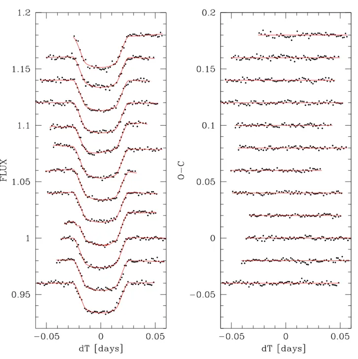
Fig. 1. Le f t : WASP-43 b transit photometry (12 first TRAPPIST transits) used in this work, binned per 2 min, period-folded on

the best-fit transit ephemeris deduced from our global MCMC analysis (see Sec. 3.3), and shifted along the y-axis for clarity. The best-fit baseline+transit models are superimposed on the light curves. The fifth and ninth models (from the top) show some wiggles because of their position-dependent terms. Right: best-fit residuals for each light curve binned per interval of 2 min.

applied. Each of the 241 exposures was composed of 17 integra-tions of 1.7s.

After a standard calibration of the images (dark-subtraction, flatfield correction), a cosmetic correction was applied. This cor-rection was done independently for each image and based on an automatic detection of the stars followed by a detection of out-lier pixels. This latter was based on a comparison of the value of each pixel to the median value of the eight adjacent pixels. For a pixel within a stellar aperture, a detection threshold of 50-σ was used, while it was 5-σ for the background pixels. Outlier pixels had their value replaced by the median value of the

ad-jacent pixels. At this stage, aperture photometry was performed with DAOPHOT for the target and comparison stars, and differ-ential photometry was obtained for WASP-43. Table 1 presents the logs of our HAWK-I observations, while Fig. 3 shows the resulting light curves with their best-fit models.

2.5.Euler/CORALIEspectra and radial velocities

We gathered eight new spectroscopic measurements of WASP-43 with the CORALIE spectrograph mounted on Euler. The spec-troscopic measurements were performed between 2011 Feb 02

(5)

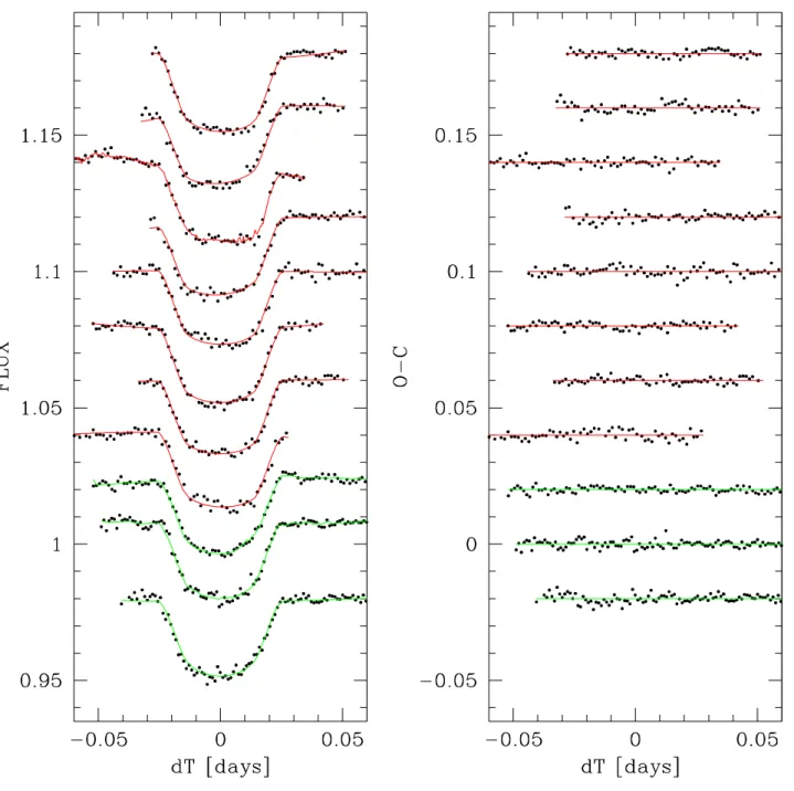
Fig. 2. Le f t : WASP-43 b transit photometry (8 last TRAPPIST transits + the 3 Euler transits) used in this work, binned per 2 min,

period-folded on the best-fit transit ephemeris deduced from our global MCMC analysis (see Sec. 3.3), and shifted along the y-axis for clarity. The best-fit baseline+transit models are superimposed on the light curves (red = TRAPPIST I + z filter; green = Euler Gunn-r′filter). The third, ninth and tenth models (from the top) show some wiggles because of their position-dependent terms.

Right: best-fit residuals for each light curve binned per interval of 2 min.

and March 12, the integration time being 30 min for all of them. RVs were computed from the calibrated spectra by weighted cross-correlation (Baranne et al. 1996) with a numerical spec-tral template. They are shown in Table 2. We analyzed these new RVs globally with the RVs presented in H11 and with our eclipse photometry (see Sec. 3.3).

3. Data analysis

Our analysis of the WASP-43 data was divided in two steps. In a first step, we performed individual analyses of the 30 eclipse light curves, determining independently for each light curves the corresponding eclipse and physical parameters. The aim of this first step was searching for potential variability among the eclipse parameters (Sec. 3.2). We then performed a global anal-ysis of the whole data set, including the RVs, with the aim to

(6)

Fig. 3. Le f t : WASP-43 b occultation photometry, binned per intervals of 2 min, period-folded on the best-fit transit ephemeris

deduced from our global MCMC analysis (see Sec. 3.3), and shifted along the y-axis for clarity. The best-fit baseline+occultation models are superimposed on the light curves (blue = TRAPPIST z′_{-filter; green = I NB1190 filter; red =}

VLT/HAWK-I NB2090 filter). Right: same light curves divided by their best-fit baseline models. The corresponding best-fit occultation models are superimposed.

obtain the strongest constraints on the system parameters (Sec. 3.3).

3.1. Method and models

Our data analysis was based on the most recent version of our adaptive Markov Chain Monte-Carlo (MCMC) algorithm (see Gillon et al. 2010 and references therein). To summa-rize, MCMC is a Bayesian stochastic simulation algorithm de-signed to deduce the posterior Probability Distribution Functions

(PDFs) for the parameters of a given model (e.g. Gregory 2005, Carlin & Louis 2008). Our implementation of the algorithm assumes as model for the photometric time-series the eclipse model of Mandel & Agol (2002) multiplied by a baseline model aiming to represent the other astrophysical and instrumental mechanisms able to produce photometric variations. For the RVs, the model is based on Keplerian orbits added to a model for the stellar and instrumental variability. Our global model can include any number of planets, transiting or not. For the RVs obtained during a transit, a model of the Rossiter-McLaughlin

(7)

Time RV σRV BS (BJDT DB-2,450,000) (km s−1) (m s−1) (km s−1) 5594.848273 -3.921 21 0.021 5604.730390 -4.149 19 0.052 5605.677373 -3.862 15 0.044 5626.663879 -4.123 18 0.035 5627.670365 -3.759 21 –0.039 5628.713064 -3.059 18 0.061 5629.686781 -3.388 17 –0.009 5632.715791 -3.126 22 0.115

Table 2. CORALIE radial-velocity measurements for WASP-43

(BS = bisector spans).

effect is also available (Gim´enez, 2006). Comparison between two models can be performed based on their Bayes factor, this latter being the product of their prior probability ratio multiplied by their marginal likelihood ratio. The marginal likelihood ra-tio of two given models is estimated from the difference of their Bayesian Information Criteria (BIC; Schwarz 1978) which are given by the formula:

BIC = χ2+ k log(N) (1)

where k is the number of free parameters of the model, N is the number of data points, and χ2 _{is the smallest chi-square found}

in the Markov chains. From the BIC derived for two models, the corresponding marginal likelihood ratio is given by e−∆BIC/2_.

For each planet, the main parameters that can be randomly perturbed at each step of the Markov chains (called jump

param-eters) are

– the planet/star area ratio dF = (Rp/R⋆)2, Rp and R⋆ being

respectively the radius of the planet and the star;

– the occultation depth(s) (one per filter) dFocc;

– the parameter b′ _{= a cos i}_p_/_R_⋆ _{which is the transit impact}

parameter in case of a circular orbit, a and ipbeing respec-tively the semi-major axis and inclination of the orbit;

– the orbital period P;

– the time of minimum light T0(inferior conjunction);

– the two parameters √e cos ω and √e sin ω, e being the

or-bital eccentricity and ω being the argument of periastron;

– the transit width (from first to last contact) W;

– the parameter K2 = K√_{1 − e}2_P1/3_{, K being the RV orbital}

semi-amplitude;

– the parameters √v sin I⋆cos β and

√

v sin I⋆sin β, v sin I⋆

and β being respectively the projected rotational velocity of the star and the projected angle between the stellar spin axis and the planet’s orbital axis.

Uniform or normal prior PDFs can be assumed for the jump and physical parameters of the system. Negative values are not al-lowed for dF, dFocc, b′, P, T0, W and K2.

Two limb-darkening laws are implemented in our code, quadratic (two parameters) and non-linear (four parameters). For each photometric filter, values and error bars for the limb-darkening coefficients are interpolated in Claret & Bloemen’s tables (2011) at the beginning of the analysis, basing on input values and error bars for the stellar effective temperature Teff,

metallicity [Fe/H] and gravity log g. For the quadratic law, the two coefficients u1 and u2 are allowed to float in the MCMC,

using as jump parameters not these coefficients themselves but

Filter u1 u2

I+z N(0.440, 0.0352₎ _{N(0.180, 0.025}2₎ Gunn-r′ _{N(0.625, 0.015}2₎ _{N(0.115, 0.010}2₎

Table 3. Prior PDF used in this work for the quadratic

limb-darkening coefficients.

the combinations c1 = 2 × u1+ u2and c2= u1− 2 × u2to

mini-mize the correlation of the obtained uncertainties (Holman et al. 2006). In this case, the theoretical values and error bars for u1

and u2deduced from Claret’s tables can be used in normal prior

PDFs. In all our analyses, we assumed a quadratic law and let u1

and u2float under the control of the normal prior PDFs deduced

from Claret & Bloemen’s tables. For the non-standard I + z fil-ter, the modes of the normal PDFs for u1and u2 were taken as

the averages of the values interpolated from Claret’s tables for the standard filters Ic and z′_{, while the errors were computed as}

the quadratic sums of the errors for these two filters. The prior PDFs deduced for WASP-43 are shown in Table 3. They were computed for Teff= 4400 ± 200K, log g = 4.5 ± 0.2 and [Fe/H] = −0.05 ± 0.17 (H11).

At the first step of the MCMC, the timings of the measure-ments are passed to the BJDT DB time standard, following the recommendation of Eastman et al. (2010) that outlined that the commonly-used BJDUT Ctime standard is not practical for high-precision timing monitoring as it drifts with the addition of one leap second roughly each year.

At each step of the Markov Chains, the stellar density is derived from Kepler’s third law and the jump parameters dF,

b′, W, √e cos ω and √e sin ω (Seager & Mallen-Ornelas 2003,

Winn 2010). Using as input values the resulting stellar density and values for Te f f and [Fe/H] drawn from their prior distri-butions, a modified version of the stellar mass calibration law deduced by Torres et al. (2010) from well-constrained detached binary systems (see Gillon et al. 2011b for details) is used to de-rive the stellar mass. The stellar radius is then dede-rived from the stellar density and mass. At this stage, the physical parameters of the planet (mass, radius, semi-major axis) are deduced from the jump parameters and stellar mass and radius. Alternatively, a value and error for the stellar mass can be imposed at the start of the MCMC analysis, In this case, a stellar mass value is drawn from the corresponding normal distribution at each step of the Markov Chains, allowing the code to deduce the other physical parameters. We preferred here to use this second op-tion, as WASP-43 was potentially lying at the lower edge of the mass range for which the calibration law of Torres et al. is valid, ∼ 0.6M⊙.

If measurements for the rotational period of the star and for its projected rotational velocity are available, they can be used in addition to the stellar radius values deduced at each step of the MCMC to derive a posterior PDF for the inclination of the star (Watson et al. 2010, Gillon et al. 2011b). We did not use this option here despite that the rotational period of the star was determined from WASP photometry to be 15.6 ± 0.4 days (H11), because the V sin I_∗ _{measurement presented by H11 (4.0 ± 0.4} km s−1_{) was presented by these authors as probably affected by}

a systematic error due to additional broadening of the lines. Several chains of 100,000 steps were performed for each analysis, their convergences being checked using the statisti-cal test of Gelman and Rubin (1992). After election of the best model for a given light curve, a preliminary MCMC analysis was performed to estimate the need to rescale the photometric

(8)

errors. The standard deviation of the residuals was compared to the mean photometric errors, and the resulting ratios βw were stored. βw represents the under- or overestimation of the white noise of each measurement. On its side, the red noise present in the light curve (i.e. the inability of our model to represent per-fectly the data) was taken into account as described by Gillon et al. (2010), i.e. a scaling factor βrwas determined from the stan-dard deviations of the binned and unbinned residuals for differ-ent binning intervals ranging from 5 to 120 minutes, the largest values being kept as βr. At the end, the error bars were mul-tiplied by the correction factor CF = βr × βw. For the RVs, a ‘jitter’ noise could be added quadratically to the error bars after the election of the best model, to equal the mean error with the standard deviation of the best-fit model residuals. In this case, it was unnecessary.

Our MCMC code can model very complex trends for the photometric and RV time-series, with up to 46 parameters for each light curve and 17 parameters for each RV time-series. Our strategy here was first to fit a simple orbital/eclipse model and to analyze the residuals to assess any correlation with the external parameters (PSF width, time, position on the chip, line bisector, etc.), then to use the Bayes factor as indicator to find the optimal baseline function for each time-series, i.e. the model minimiz-ing the number of parameters and the level of correlated noise in the best-fit residuals. For ground-based photometric time-series, we did not use a model simpler than a quadratic polynomial in time, as several effects (color effects, PSF variations, drift on the chip, etc) can distort slightly the eclipse shape and can thus lead to systematic errors on the deduced transit parameters. This is especially important to include a trend in the baseline model for transit light curve with no out-of-transit data before or af-ter the transit, and/or with a small amount of out-of-transit data. Having a rather small amount of out-of-transit data is quite com-mon for ground-based transit photometry, as the target star is visible under good conditions (low airmass) during a limited du-ration per night. In such conditions, an eclipse model can have enough degrees of freedom to compensate for a small-amplitude trend in the light curve, leading to an excellent fit but also to bi-ased results and overoptimistic error bars. Allowing the MCMC to ‘twist’ slightly the light curve with a quadratic polynomial in time compensates, at least partially, for this effect.

For the RVs, our minimal baseline model is a scalar Vγ

repre-senting the systemic velocity of the star. It is worth noticing that most of the baseline parameters are not jump parameters in the MCMC, they are deduced by least-square minimization from the residuals at each step of the chains, thanks to their linear nature in the baseline functions (Bakos et al. 2009, Gillon et al. 2010).

3.2. Individual analysis of the eclipse time-series

As mentioned above, we first performed an independent analysis of the transits and occultations aiming to elect the optimal model for each light curve and to assess the variability and robustness of the derived parameters. For all these analyses, the orbital pe-riod and eccentricity were kept respectively to 0.813475 days and zero (H11), and the normal distribution N(0.58, 0.052_{) M}

⊙

(H11) was used as prior PDF for the stellar mass. For the transit light curves, the jump parameters were dF, b′_{, W and T}₀_{. For the}

occultations, the only jump parameter was the occultation depth

dFocc, the other system parameters being drawn at each step of the MCMC from normal distributions deduced from the values + errors derived in H11.

Table 1 presents the baseline function selected for each light curve, the derived factors βw, βr, CF, and the standard deviation

of the best-fit residuals, unbinned and binned per 120s. These results allow us to assess the photometric precision of the used instruments.The TRAPPIST data show mean values for βwand βrvery close to 1, the I+z data having < βw>=1.03 and < βr >= 1.05, while the z′data have < βw >= 0.98 and < βr >= 1.11. This suggests that the photometric errors of each measurement are well approximated by a basic error budget (photon, read-out, dark, background, scintillation noises), and that the level of correlated noise in the data is small. Furthermore, we notice that most TRAPPIST light curves are well modeled by the ‘minimal model’, i.e. the sum of an eclipse model and a quadratic trend in time. Only one TRAPPIST transit light curve requires additional terms in x and y, while one occultation light curve acquired when the moon was close to full requires a linear term in background. The mean photometric errors per 2 min intervals can also be considered as very good for a 60cm telescope monitoring a V = 12.4 star: 0.11% and 0.15% in the I +z and z′_{filters, respectively,}

which is similar to the mean photometric error of Euler data, 0.12%. Euler data show also small mean values of < βw >= 1.27 and < βr >= 1.05. Their modeling requires PSF position terms for 2 out of 3 eclipses, despite the good sampling of the PSF and the active guiding system keeping the stars nearly on the same pixels. This could indicate that the flatfields’ quality is perfectible.

For the first HAWKI light curve, taken in the NB2090 filter, we notice that we have to account for a ‘ramp’ effect (the log(t) term) similar to the well-documented sharp variation of the ef-fective gain of the Spitzer/IRAC detector at 8 µm (e.g. Knutson et al. 2008), and also for a dependance of the measured flux with the exact position of the PSF center on the chip. This position effect could be decreased by spreading the flux on more pixels (defocus), but this would also increase the background’s contri-bution to the noise budget, potentially bringing not only more white noise but also some correlation of the measured counts with the variability of the local thermal structure. The photomet-ric quality reached by these NB2090 data (βr= 1.09, mean error of 360 ppm per 2 min time interval), can be judged as excellent. For the NB1190 HAWKI data, we had to include a dependance in the PSF width in the model. This is not surprising, consider-ing the large variability of the seeconsider-ing durconsider-ing the run. We also no-tice for these data that our error budget underestimated strongly the noise of the measurements (βw = 2.22), suggesting an un-accounted noise source. Still, the reached photometric quality remains excellent (βr= 1, mean error of 470 ppm per 2 min time interval).

Table 4 presents for each eclipse light curve the values and errors deduced for the jump parameters. Several points can be noticed.

– The emission of the planet is clearly (10-σ) detected at 2.09 µ_{m. At 1.19 µm, it is barely detected (∼ 2.3-σ). It is not} detected in any of the z′_{-band light curves.}

– The transit shape parameters b′_{, W, and dF, show scatters}

slightly larger than their average error, the corresponding ra-tio being, respectively, 1.24, 1.26, and 1.54. Furthermore, these parameters show significant correlation, as can be seen in Fig. 4.

– Fitting a transit ephemeris by linear regression with the

measured transit timings shown in Table 4, we ob-tained T (N) = _{2, 455, 528.868289(±0.000072) + N ×} 0.81347728(±0.00000060) BJDT DB. Table 4 shows (last col-umn) the resulting transit timing residuals (observed minus computed, O-C). Fig. 5 (upper panel) shows them as a func-tion of the transit epochs. The scatter of these timing

(9)

resid-uals is 2.1 times larger than the mean error, 18s. No clear pattern is visible in the O-C diagram.

The apparent variability of the four transit parameters is present in both TRAPPIST and Euler results. The correlation of the de-rived transit parameters is not consistent with actual variations of these parameters and favors biases from instrumental and/or astrophysical origin. This apparent variability of the transit pa-rameters could be explained by the variability of the star itself. Indeed, WASP-43 is a spotted star (H11), and occulted spots (and faculae) can alter the observed transit shape and bias the measured transit parameters (e.g. Huber et al. 2011, Berta et al. 2011). We do not detect clear spot signatures in our light curves, but our photometric precision could be not high enough to de-tect such low-amplitude structures, so we do not reject this hy-pothesis. On their side, unocculted spots should have a negligi-ble impact on the measured transit depths, considering the low amplitude of the rotational photometric modulation detected in WASP data (6 ± 1 mmag). Still, they could alter the slope of the photometric baseline and make it more complex. We represent this baseline as an analytical function of several external param-eters in our MCMC simulations, but the unavoidable inaccuracy of the chosen baseline model can also bias the derived results. As described in Sec. 2.1, no pointing corrections were applied dur-ing the TRAPPIST runs because of a stellar catalogue problem. Even if the resulting drifts did not introduce clear correlations of the measured fluxes with PSF positions, they could have slightly affected the shape of the transits. These considerations reinforce the interest of performing global analysis of extensive data sets (i.e. many eclipses) in order to minimize systematic errors and to reach high accuracies on the derived parameters.

3.3. Global analysis of photometry and radial velocities

The global MCMC analysis of our data set was divided in three steps. For each step of the analysis, the MCMC jump parameters were dF, W, b′_{, T}₀_{, P,} √_{e cos ω,} √_{e sin ω, three dF}_occ_{(for the}

z′_{, NB1190, and NB2090 filters), K}

2, and the limb-darkening

co-efficients c1and c2for the I + z and Gunn-r′filters. No model for

the Rossiter-McLaughlin was included in the global model, as no RV was obtained at the transit phase. For each light curve, we as-sumed the same baseline model than for the individual analysis. The assumed baseline for the RVs was a simple scalar (systemic velocity Vγ).

In a first step, we performed a chain of 100,000 steps with the aim to redetermine the scaling factors of the photometric er-rors. The deduced values are shown in Table 1. It can be noticed that the mean < βr>for the 20 transits observed by TRAPPIST in I + z filter is now 1.52, for 1.05 after the individual analysis of the lightcurves. We notice the same tendency for the Euler Gunn-r′_{transits: < βr}_>_{goes up from 1.05 to 1.42. Considering}

the apparent variability of the transit parameters deduced from the individual analysis of the light curves and their correlations, our interpretation of this increase of the < βr >is that a part of the correlated noise (from astrophysical source or not) of a tran-sit light curve can be ‘swallowed’ in the trantran-sit+baseline model, leading to a good fit in terms of merit function but also to bi-ased derived parameters. By relying on the assumption that all transits share the same profile, the global analysis allows to bet-ter separate the actual transit signal from the correlated noises of similar frequencies, leading to larger < βr >values. It is also worth noticing that the < βr >for the transits, 1.50, is larger than the one for the occultations, 1.12, which is consistent with the crossing of spots by the planet during transit, but can also

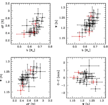
Fig. 4. Correlation diagrams for the transit parameters deduced

from the individual MCMC analysis of the 23 transit light curves. Top left: transit depth vs transit impact parameter. Top

right: transit duration vs transit impact parameter. Bottom left:

transit duration vs transit depth. Bottom right: TTV (observed minus calculated transit timing) vs transit duration. The filled black and open red symbols correspond, respectively, to the TRAPPIST and Euler light curves.

Epoch 0 50 100 150 200 250 -2 -1 0 1 2 Epoch 0 50 100 150 200 250 -2 -1 0 1 2

Fig. 5. T op: Observed minus calculated transit timings obtained

from the individual analysis of the transit light curves as a func-tion of the transit epoch. The filled black and open red sym-bols correspond, respectively, to the TRAPPIST and Euler light curves. Bottom: same but deduced from the global analysis of all transits.

(10)

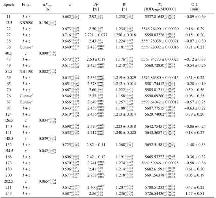
Epoch Filter dFocc b dF W T0 O-C [%] [%] [h] [BJDT DB-2450000] [min] 11 I + z 0.682+0.028 −0.035 2.92 +0.14 −0.13 1.250 +0.038 −0.034 5537.81648 +0.00043 −0.00048 −0.09 ± 0.69 13.5 NB2090 0.156+0.015 −0.016 22 I + z 0.673+0.030 −0.036 2.50 +0.10 −0.11 1.234 +0.024 −0.029 5546.76490 ± 0.00020 0.16 ± 0.29 27 I + z 0.716+0.019 −0.021 2.721 ± 0.077 1.250 ± 0.018 5550.83228 +0.00014 −0.00013 0.15 ± 0.20 38 I + z 0.645+0.043 −0.052 2.43 +0.11 −0.09 1.224 +0.029 −0.026 5559.78038 ± 0.00021 −0.07 ± 0.30 38 Gunn-r′ _0.640+0.035 −0.041 2.423 +0.088 −0.083 1.181 +0.019 −0.020 5559.78092 ± 0.00016 0.71 ± 0.22 40.5 z′ _0.090+0.061 −0.053 43 I + z 0.573+0.043 −0.047 2.60 ± 0.17 1.176 +0.022 −0.024 5563.84773 ± 0.00023 −0.12 ± 0.33 49 I + z 0.611+0.042 −0.048 2.425 +0.090 −0.079 1.210 +0.020 −0.021 5568.72830 +0.00018 −0.00017 −0.54 ± 0.26 51.5 NB1190 0.082+0.035 −0.037 59 I + z 0.643+0.022 −0.027 2.534 +0.067 −0.070 1.219 ± 0.029 5576.86380 ± 0.00015 0.51 ± 0.22 65 I + z 0.651+0.025 −0.030 2.378 +0.064 −0.060 1.212 ± 0.014 5581.74412 +0.00012 −0.00013 −0.28 ± 0.19 70 I + z 0.667+0.026 −0.032 2.60 +0.24 −0.22 1.222 +0.041 −0.038 5585.81211 +0.00039 −0.00038 0.59 ± 0.56 76 Gunn-r′ _0.546+0.058 −0.073 2.37 +0.10 −0.09 1.158 +0.023 −0.020 5590.69260 +0.00017 −0.00016 0.05 ± 0.25 87 Gunn-r′ _0.656+0.030 −0.037 2.649 +0.089 −0.087 1.257 +0.019 −0.020 5599.64042 ± 0.00017 −0.57 ± 0.25 97 I + z 0.643+0.032 −0.041 2.456 +0.068 −0.075 1.188 +0.017 −0.018 5607.77515 +0.00014 −0.00015 −0.63 ± 0.22 124 I + z 0.619+0.028 −0.029 2.456 +0.064 −0.059 1.213 ± 0.014 5629.74002 +0.00014 −0.00013 0.79 ± 0.20 126.5 z′ _0.034+0.033 −0.023 140 I + z 0.698+0.020 −0.024 2.570 +0.070 −0.072 1.223 ± 0.018 5642.75451 +0.00016 −0.00017 −0.86 ± 0.25 141 I + z 0.633+0.029 −0.037 2.712 +0.093 −0.094 1.240 ± 0.020 5643.56871 +0.00019 −0.00018 0.18 ± 0.27 148.5 z′ _0.039+0.042 −0.027 152 I + z 0.725+0.023 −0.027 2.82 ± 0.11 1.268 +0.024 −0.023 5652.51581 +0.00021 −0.00023 −1.48 ± 0.33 154.5 z′ _0.042+0.050 −0.029 168 I + z 0.606+0.033 −0.036 2.42 ± 0.12 1.191 +0.018 −0.016 5665.53222 +0.00022 −0.00021 −0.36 ± 0.32 173 I + z 0.670+0.029 −0.030 2.741 +0.098 −0.084 1.274 +0.029 −0.026 5669.59946 ± 0.00025 −0.58 ± 0.36 189 I + z 0.596+0.051 −0.072 2.41 +0.10 −0.11 1.214 +0.024 −0.026 5682.61592 +0.00020 −0.00021 0.61 ± 0.30 200 I + z 0.677+0.017 −0.021 2.738 +0.060 −0.070 1.218 +0.016 −0.015 5691.56378 +0.00013 −0.00012 0.05 ± 0.19 202.5 z′ _0.065+0.054 −0.044 211 I + z 0.642+0.022 −0.031 2.400 +0.067 0.073 1.207 +0.014 −0.017 5700.51232 +0.00015 −0.00014 0.47 ± 0.22 243 I + z 0.687+0.047 −0.052 2.56 +0.19 −0.16 1.236 +0.050 −0.043 5726.54436 +0.00056 −0.00044 1.57 ± 0.81

Table 4. Median and 1-σ errors of the posterior PDFs deduced for the jump parameters from the individual analysis of the eclipse

light curves. For each light curve, this table shows the epoch based on the transit ephemeris presented in H11, the filter, and the derived values for the occultation depth, impact parameter, transit depth, transit duration, and transit time of minimum light. The last column shows for the transits the difference (and its error) between the measured timing and the one deduced from the best-fitting transit ephemeris computed by linear regression, T (N) = 2455528.868289(0.000072) + N × 0.81347728(0.00000060) BJDT DB.

be explained by the much larger number of transits than occul-tations.

In a second step, we used the updated error scaling factors and performed a MCMC of 100,000 steps to derive the marginal-ized PDF for the stellar density ρ⋆. This PDF was used as input

to interpolate stellar tracks. As in Hebb et al. (2009), we used ρ−1/3_⋆ , mostly for practical reasons. Other inputs were the stel-lar effective and metallicity derived by H11, Teff = 4400 ± 200

K and [Fe/H] = -0.05 ± 0.17 dex. Those parameters were as-sumed distributed as a Gaussian. For each ρ−1/3_⋆ value from the MCMC, a random Gaussian value was drawn for stellar param-eters. That point was placed among the Geneva stellar evolu-tion tracks (Mowlavi et al. 2012) that are available in a grid fine enough to allow an MCMC to wander without computational systematic effects; a mass and age were interpolated. If the point fell off the tracks, it was discarded. Because of the way stars

be-have at these small masses, within the (ρ−1/3⋆ , Teff, [Fe/H]) space,

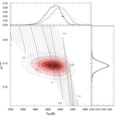
the parameter space over which the tracks were interpolated cov-ered stellar ages well above a Hubble time. A restriction on the age was therefore added. Only taking ages < 12 Gyr, we obtained the distribution as shown in Fig. 6, refining the stellar parame-ters to Teff= 4520 ± 120 K and [Fe/H] = -0.01 ± 0.12 dex. The

stellar mass is estimated to M⋆= 0.717 ± 0.025M_⊙. The output

distribution is very close to Gaussian as displayed in Fig. 6. In addition the output ρ−1/3_⋆ distribution has not been affected. Thus, our strongly improved precision on the stellar density combined with a constraint on the age (to be younger than a Hubble time) allows us to reject the main stellar solution proposed by H11 (M⋆= 0.58 ± 0.05M⊙). Because the allowed (ρ−1/3⋆ , Teff, [Fe/H])

space within the tracks still covers quite a large area, it is impos-sible at the moment to constrain the stellar age. The process is described in Triaud 2011 (PhD thesis).

(11)

Fig. 6. Main panel: modifield Herztsprung-Russell diagram

showing the posterior PDF of ρ−1/3_⋆ as a function of Teff after

interpolating with the Geneva stellar evolution tracks for stars on the main sequence. Masses are indicated and correspond to the bold tracks. The solid, dashed and dotted lines correspond to the 1-σ, 2-σ and 3-σ contours, respectively. Secondary

pan-els: marginalised PDF of ρ−1/3_⋆ and Teff. In both panels, there are

three histograms: dotted: input distribution; grey: output distri-bution; black: output distribution for ages < 12 Gyr.

Fig. 8. Euler/CORALIE RV measurements period-folded on the

best-fit transit ephemeris from the global MCMC analysis, cor-rected for the systemic RV, with the best-fit orbital model over-imposed.

We then performed a third MCMC step, using as prior distri-butions for M⋆, Teff, and [Fe/H], the normal distributions

match-ing the results of our stellar modelmatch-ing, i.e. N(0.717, 0.0252_{) M}

⊙,

N(4520, 1202

) K, and N(−0.01, 0.122_{) dex, respectively. The}

best-fit photometry and RV models are shown respectively in Fig. 7 and 8, while the derived parameters and 1-σ error bars are shown in Table 5.

MCMC Jump parameters

Planet/star area ratio (Rp/R⋆)2[%] 2.542+0.024_−0.025

b′_{= a cos i} p/R⋆[R⋆] 0.656 ± 0.010 Transit width W [h] 1.2089+0.0055 −0.0050 T0− 2450000 [BJDT DB] 5726.54336 ± 0.00012 Orbital period P [d] _{0.81347753 ± 0.00000071} RV K2[m s−1d1/3] 511.5+5.1_−5.0 √ e cos ω 0.020+0.022 −0.023 √ e sin ω −0.025+0.066 −0.064 dFocc,z′[ppm] 210+190 −130, < 850 (3-σ) dFocc,N B1190 790+320₋₃₁₀, < 1700 (3-σ) dFocc,N B2090 1560 ± 140 c1I+z 0.983 ± 0.050 c2I+z 0.065 ± 0.060 c1r′ 1.363 ± 0.047 c2r′ 0.401 ± 0.051

Deduced stellar parameters

u1I+z 0.406 ± 0.026 u2I+z 0.171 ± 0.024 u1r′ 0.625 ± 0.024 u2r′ 0.112 ± 0.020 Vγ[km s−1] −3.5950 ± 0.0040 Density ρ⋆[ρ⊙] 2.410+0.079_−0.075

Surface gravity log g⋆[cgs] 4.645+0.011_−0.010

Mass M⋆[M_⊙] 0.717 ± 0.025

Radius R⋆[R⊙] 0.667+0.010_−0.011

Teff[K]a 4520 ± 120

[Fe/H] [dex]a

−0.01 ± 012 Deduced planet parameters

RV K [ m s−1_] _547.9+5.5 −5.4 Rp/R⋆ 0.15945+0.00076_−0.00077 btr[R⋆] 0.6580+0.0089_−0.0095 boc[R⋆] 0.655+0.012_−0.013 Toc− 2450000 [BJDT DB] 5726.95069+0.00084_−0.00078

Orbital semi-major axis a [AU] _{0.01526 ± 0.00018} Roche limit aR[AU] 0.00768 ± 0.00016

a/aR 1.986+0.030_−0.029

a/R⋆ 4.918+0.053_−0.051

Orbital inclination ip[deg] 82.33 ± 0.20

Orbital eccentricity e 0.0035+0.0060

−0.0025, < 0.0298 (3-σ)

Argument of periastron ω [deg] ₋₃₂+115 −34

Equilibrium temperature Teq[K]b 1440+40₋₃₉

Density ρp[ρJup] 1.826+0.084_−0.078 Density ρp[g/cm3] 1.377+0.063_−0.059

Surface gravity log gp[cgs] 3.672+0.013_−0.012

Mass Mp[MJup] 2.034+0.052_−0.051 Radius Rp[RJup] 1.036 ± 0.019

Table 5. Median and 1-σ limits of the posterior marginalized

PDFs obtained for the WASP-43 system derived from our global MCMC analysis. a_{From stellar evolution modeling (Sect. 3.3).} b_{Assuming A=0 and F=1.}

(12)

Fig. 7. Left: TRAPPIST I + z (top) and Euler Gunn-r′(bottom) transit photometry period-folded on the best-fit transit ephemeris from the global MCMC analysis, corrected for the baseline and binned per 2 min intervals, with the best-fit transit models over-imposed. Right: same for the occultation photometry obtained by TRAPPIST in z′ filter (top), and by VLT/HAWK-I in NB1190 (middle) and NB2090 (bottom) filters, except that the data points are binned per 5 min intervals.

Global analysis of the 23 transits with free timings

As a complement to our global analysis of the whole data set, we performed a global analysis of the 23 transit light curves alone. The goal here was to benefit from the strong constraint brought on the transit shape by the 23 transits to derive more accurate transit timings and to assess the periodicity of the transit. In this analysis, we kept fixed the parameters T0 and P to the values

shown in Table 5, and we added a timing offset as jump param-eter for each transit. The orbit was assumed to be circular. The other jump parameters were dF, W, b′_{, and the limb-darkening}

coefficients c1and c2 for both filters. The resulting transit

tim-ings and their errors are shown in Table 6. Fitting a transit ephemeris by linear regression with these new derived transit timings, we obtained T (N) = 2, 455, 528.868227(±0.000078) +

N ×0.81347764(±0.00000065) BJDT DB. Table 6 shows (last col-umn) the resulting transit timing residuals (observed minus com-puted, O-C). Fig. 5 (lower panel) shows them as a function of the transit epochs. The scatter of these timing residuals is now 1.8 times larger than the mean error, 19s. Comparing the errors on the timings derived from individual and global analysis of the transit photometry, one can notice that the better constraint on the transit shape for the global analysis improves the error of a few timings, but that most of them have a slightly larger error because of the better separation of the actual transit signal from the red noise (see above).

4. Discussion

4.1. The physical parameters of WASP-43 b

Comparing our results for the WASP-43 system with the ones presented in H11, we notice that our derived parameters agree well with the second solution mentioned in H11, while being sig-nificantly more precise. WASP-43 b is thus a Jupiter-size planet,

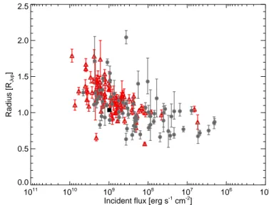
twice more massive than our Jupiter, orbiting at only ∼0.015 AU from a 0.72 M_⊙main-sequence K-dwarf. Despite having the smallest orbital distance among the hot Jupiters, WASP-43 b is far from being the most irradiated known exoplanet, because of the small size and temperature of its host star. Assuming a solar-twin host star, its incident flux ∼9.6 108_{erg s}−1_cm−2_would

cor-respond to a P = 2.63 d orbit (a = 0.0374 AU), i.e. to a rather typical hot Jupiter. With a radius of 1.04 RJup, WASP-43 b lies toward the bottom of the envelope described by the published planets in the Rp vs. incident flux plane (Fig. 9). Taking into account its level of irradiation, the high density of the planet favors an old age and a massive core under the planetary struc-ture models of Fortney et al. (2010). Our results are consistent with a circular orbit, and we can put a 3-σ upper limit <0.03 to the orbital eccentricity. Despite its very short period, WASP-43 b has a semi-major axis approximatively twice larger than its Roche limit aR, which is typical for hot Jupiters (Ford & Rasio 2006, Mastumura et al. 2010). As noted by these authors, the inner edge of the distribution of most hot Jupiters at ∼2 aR fa-vors migrational mechanisms based on the scattering of planets on much wider orbit and the subsequent tidal shortening and cir-cularization of their orbits. Thus, WASP-43 b does not appear to be a planet exceptionally close to its final tidal disruption, unlike WASP-19 b that orbits at only 1.2 aR(Hellier et al. 2011a).

4.2. The atmospheric properties of WASP-43 b

We have modeled the atmosphere of WASP-43 b using the meth-ods described in Fortney et al. (2005, 2008) and Fortney & Marley (2007). In Fig. 10, we compare the planet-to-star flux ratio data to three atmosphere models. The coldest model (or-ange) uses a dayside incident flux decreased by 1/2 to simulate the loss of half of the absorbed flux to the night side of the planet. Clearly the planet is much warmer than this model. In blue and

(13)

Epoch Filter Ttr O-C [BJDT DB-2450000] [min] 11 I + z 5537.81673+0.00047 −0.00046 0.36 ± 0.68 22 I + z _{5546.76494 ± 0.00022} _{0.30 ± 0.32} 27 I + z 5550.83219+0.00015 −0.00016 0.10 ± 0.23 38 I + z _{5559.78033 ± 0.00021} −0.07 ± 0.30 38 Gunn-r′ _5559.78078+0.00016 −0.00017 0.58 ± 0.24 43 I + z _{5563.84771 ± 0.00022} −0.08 ± 0.32 49 I + z _{5568.72836 ± 0.00015} −0.39 ± 0.22 59 I + z 5576.86380+0.00016 −0.00015 0.57 ± 0.23 65 I + z _{5581.74410 ± 0.00020} −0.25 ± 0.29 70 I + z 5585.81205+0.00021 −0.00022 0.56 ± 0.32 76 Gunn-r′ _{5590.69259 ± 0.00018} _{0.09 ± 0.26} 87 Gunn-r′ _5599.64043+0.00026 −0.00025 −0.51 ± 0.37 97 I + z _{5607.77517 ± 0.00014} −0.56 ± 0.20 124 I + z 5629.73995+0.00019 −0.00018 0.71 ± 0.27 140 I + z _{5642.75450 ± 0.00015} −0.86 ± 0.22 141 I + z _{5643.56872 ± 0.00028} _{0.21 ± 0.40} 152 I + z 5652.51586+0.00024 −0.00025 −1.39 ± 0.36 168 I + z 5665.53229+0.00019 −0.00018 −0.26 ± 0.27 173 I + z _{5669.59976 ± 0.00023} −0.14 ± 0.33 189 I + z 5682.61584+0.00022 −0.00023 0.49 ± 0.33 200 I + z 5691.56383+0.00022 −0.00023 0.11 ± 0.33 211 I + z 5700.51237+0.00014 −0.00015 0.52 ± 0.22 243 I + z _{5726.54399 ± 0.00035} _{1.00 ± 0.50}

Table 6. Median and 1-σ errors of the posterior PDFs

de-duced for the timings of the transits from their global analy-sis. The last column shows the difference (and its error) be-tween the measured timing and the one deduced from the best-fitting transit ephemeris computed by linear regression, T (N) = 2455528.868227(0.000078) + N × 0.81347764(0.00000065) BJDT DB.

red are two models where the dayside incident flux is increased by a factor of 4/3 to simulate zero redistribution of absorbed flux (see, e.g., Hansen 2008). The red model features a dayside tem-perature inversion due to the strong optical opacity of TiO and VO gases (Hubeny et al. 2003, Fortney et al. 2006). The blue model is run in the same manner as the red model, but TiO and VO opacity are removed.

The blue and red models are constructed to maximize the emission from the dayside of the planet. Figure 10 shows that only such bright models could credibly match the data points. While a dayside with no temperature inversion is slightly favored by the 1.2 µm data point, it is difficult to come to a firm conclu-sion. Day-side emission measurements from Warm Spitzer will help to better constrain the atmosphere as well. They will also allow getting an even smaller upper-limit on the orbital eccen-tricity.

Fortney et al. model fits to near infrared photometry of other transiting planets (e.g., Croll et al. 2010) have generally fa-vored inefficient temperature homogenization between the day and night hemispheres, although the warm dayside of WASP-43 b appears to be at the most inefficient end of this contin-uum. The apparent effeciency of temperature homogenization is expected to vary with wavelength. In particular, near infrared

1011 1010 109 108 107 106 105

Incident flux [erg s-1

cm-2 ] 0.0 0.5 1.0 1.5 2.0 2.5 Radius [R Jup ]

Fig. 9. Planetary radii as a function of incident flux.

WASP-43 b is shown as a black square. Grey filled circles are

Kepler planetary candidates (see Demory & Seager 2011).

Transiting giant planets previously published, and mostly from ground-based surveys, are shown as grey triangles. The rel-evant parameters Rp, Rs, Te f f and a have been drawn from http://www.inscience.ch/transits on August 29, 2011.

Fig. 10. Model planet-to-star flux ratios compare to the three

data points. The data are green diamonds with 1−σ error bars shown. The orange model assumes planet-wide redistribution of absorbed flux. The red and blue models assume no redistribution of absorbed flux, to maximize the day-side temperature. The red model includes gaseous TiO and VO and has a temperature in-version. [See the figure inset.] The blue and orange models have TiO and VO opacity removed, and do not have a temperature inversion. For each model, filled circles are model fluxes aver-aged over each bandpass. The data slightly favor a model with no day-side temperature inversion.

bands, at minima in water vapor opacity, are generally expected to probe deeper into atmospheres than the Spitzer bandpasses.

4.3. Transit timings

Dynamical constraints can be placed on short orbits companion planets from the 23 transits obtained in this study. The linear fit

(14)

2 3 4 5 Orbital Period [days]

0.1 1.0 10.0 100.0 1000.0 10000.0 Detectable Mass [M Earth ]

Fig. 11. Detectivity domain for a putative WASP-43 c planet,

as-suming ec= 0 (black) and ec= 0.05 (red). The solid curves de-limit the mass-period region where planets yield maximum TTV on WASP-43 b above 114 s (3-σ detection based on the present data). The dotted curves show the 1-σ threshold. Nearly hori-zontal solid, dashed and dotted lines shows RV detection limits for RV semi-amplitude K=5, 10 and 15 m s−1_{respectively.}

to the transit timings described above yields a reduced χ2_{of 4.6}

and the rms of its residuals is 38s. Two transits (epochs 140 and 152) have a O-C different from zero at the ∼4-σ level. The most plausible explanation for the significant scatter observed in the transit timings is systematic errors on the derived timings due to the influence of correlated noise. Another potential explanation is asymmetries in the transit light curves caused by the crossing of one or several star spots by the planet. In such cases, the fitted transit profile is shifted with time, producing timing variations.

We also explored the detectability domain of a second planet in the WASP-43 system. To this end, we followed Agol et al. (2005) and used the Mercury n-body integrator package (Chambers 1999). We simulated 3-body systems including a sec-ond companion with orbital periods ranging between 1.3 and 50 days, masses from 0.1 M_⊕ to 2.0 MJup and an orbital ec-centricities of ec = 0 and ec = 0.05. For each simulation, we computed the rms of the computed transits timings variations. The results are shown on Fig.11 where the computed 1-σ (red) and 3-σ (black) detection thresholds are plotted for each point in the mass-period plane. We also added RV detectability threshold curves based on 5 (solid), 10 (dash) and 15 (dot) m s−1

semi-amplitudes (K).

Based on the present set of timings, the timings variations caused by a 5 Earth mass companion in 2:1 resonance would have been detected with 3-σ confidence, while unseen with ra-dial velocities alone.

5. Conclusions

In this work we have presented 23 transit light curves and 7 oc-cultation light curves for the ultra-short period planet WASP-43 b. We have also presented 8 new measurements of the ra-dial velocity of the star. Thanks to this extensive data set, we have significantly improved the parameters of the system. Notably, our strongly improved precision on the stellar den-sity (2.41 ± 0.08ρ⊙) combined with a very reasonable constraint

on its age (to be younger than a Hubble time) allowed us to break the degeneracy of the stellar solution mentioned by H11. The resulting stellar mass and size are 0.717 ± 0.025M⊙ and

0.667 ±0.011R⊙. Our deduced physical parameters for the planet

are 2.034 ± 0.052MJup and 1.036 ± 0.019RJup. Taking into ac-count its level of irradiation, the high density of the planet favors an old age and a massive core. Our deduced orbital eccentricity, 0.0035+0.0060_−0.0025, is consistent with a fully circularized orbit.

The parameters deduced from the individual analysis of the 23 transit light curves show some extra scatter that we attribute to the correlated noise of our data and, possibly, to the crossing of spots during some transits. This conclusion is based on the correlation observed among the transit parameters. These results reinforce the interest of performing global analysis of extensive data sets in order to minimize systematic errors and to reach high accuracies on the derived parameters.

We detected the emission of the planet at 2.09 µm at better than 11-σ, the deduced occultation depth being 1560 ± 140 ppm. Our detection of the occultation at 1.19 µm is marginal (790 ± 320 ppm) and more observations would be needed to confirm it. We place a 3-σ upper limit of 850 ppm on the depth of the occultation at ∼0.9 µm. Together, these results strongly favor a poor redistribution of the heat from the dayside to the nightside of the planet, and marginally favor a model with no day-side temperature inversion.

Acknowledgements. TRAPPIST is a project funded by the Belgian Fund

for Scientific Research (Fond National de la Recherche Scientifique, F.R.S-FNRS) under grant FRFC 2.5.594.09.F, with the participation of the Swiss National Science Fundation (SNF). M. Gillon and E. Jehin are FNRS Research Associates. We are grateful to ESO La Silla and Paranal staffs for their continu-ous support. We thank the anonymcontinu-ous referee for his valuable suggestions.

References

Agol, E., Steffen, J., Sari, R., & Clarkson, W. 2005, MNRAS, 359, 567 Anderson, D. R., Gillon, M., Maxted P., et al. 2010, A&A, 513, L3 Bakos, G. ´A, Torres, G., P´al, A., et al. 2009, ApJ, 710, 1724 Baranne, A., Queloz, D., Mayor, M. et al. 1996, A&AS, 119, 373 Barker, A. J. & Ogilvie, G. I. 2009, MNRAS, 395, 2268 Berta, Z. K., Charbonneau, D., Bean, J., et al. 2011, ApJ, 736, 12

Brown, D. J. A., Collier Cameron, A., Hall, C., et al. 2011, MNRAS, 415, 605 Carlin, B. P. & Louis, T. A. 2008, Bayesian Methods for Data Analysis, Third

Edition (Chapman & Hall/CRC)

Casali, M., Pirard, J.-F., Kissler-Patig, M. et al. 2006, SPIE, 6269, 29 Chambers J. E., 1999, MNRAS, 304, 793

Claret, A. & Bloemen, S. 2011, A&A, 529, A75

Croll, B., Jayawardhana, R., Fortney, J. J., Lafreni`ere, D., & Albert, L. 2010, ApJ, 718, 920

D’Angelo, G., Durisen, R. H., Lissauer, J. J. 2010, Exoplanets, ed. S. Seager, University of Arizona Press, p. 319

Demory, B.-O., & Seager, S. 2011, ApJS, 197, 12

Eastman, J., Siverd, R., & Gaudi, B. S. 2010, PASP, 122, 935 Fabrycky, D. C. & Tremaine, S. 2007, ApJ, 669, 1298 Ford, E. B. & Rasio, F. A. 2006, ApJ, 638, L45

Fortney, J. J., Marley, M. S., Lodders, K., Saumon, D., & Freedman, R. S. 2005, ApJ, 627, L69

Fortney, J. J., Saumon, D., Marley, M. S., Lodders, K., & Freedman, R. S. 2006, ApJ, 642, 495

Fortney, J. J., Marley, M. S., Barnes, J. W. 2007, ApJ, 659, 1661 Fortney, J. J. & Marley, M. S. 2007, ApJ, 666, L45

Fortney, J. J., Lodders, K., Marley, M. S., & Freedman, R. S. 2008, ApJ, 678, 1419

Gelman, A. & Rubin D. 1992, Statist. Sci., 7, 457

Gibson, N. P., Aigrain, S., Pollaco, D. L., et al. 2010, MNRAS, 404, L14 Gillon, M., Lanotte, A. A., Barman, T., et al. 2010, A&A, 511, 3

Gillon, M., Jehin, E., Magain, P., et al. 2011a, Detection and Dynamics of

Transiting Exoplanets, Proceedings of OHP Colloquium (23-27 August

2010), eds. F. Bouchy, R. F. Diaz & C. Moutou, Platypus Press Gillon, M., Doyle, A., Maxted, P., et al. 2011b, A&A, 533, A88 Gim´enez, A. 2006, ApJ, 650, 408

Gregory, P. C. 2005, Bayesian Logical Data Analysis for the Physical Sciences, Cambridge University Press

Gu, P.-G., Lin, D. N. C., Bodenheimer, P. H. 2003, ApJ, 588, 509 Hansen, B. M. S., 2008, ApJS, 179, 484