Département de Mathématiques, Faculté des Sciences
Bayesian Design Space applied to
Pharmaceutical Development
Thèse présentée en vue de l’obtention du grade de
Docteur en Sciences, orientation statistique, par:
Pierre Lebrun
Membres du Jury
Prof. Adelin Albert Dr. Bruno Boulanger
Prof. Paul Eilers Prof. Bernadette Govaerts Prof. Gentiane Haesbroeck
Prof. Philippe Hubert Prof. Philippe Lambert
Dr. John Peterson
Given the guidelines such as the Q8 document published by the International Conference on Harmonization (ICH), that describe the “Quality by Design” paradigm for the Pharmaceutical Development, the aim of this work is to provide a complete methodology addressing this problematic. As a result, various Design Spaces were obtained for different analytical methods and a manufacturing process.
In Q8, Design Space has been defined as the “the multidimensional combination and interaction of input variables (e.g., material attributes) and process parameters that have been demonstrated to provide assurance of quality” for the analytical outputs or processes involved in Pharmaceutical Development. Q8 is thus clearly devoted to optimization strategies and robustness studies.
In the beginning of this work, it was noted that existing statistical methodolo-gies in optimization context were limited as the predictive framework is based on mean response predictions. In such situations, the data and model uncertainties are generally completely ignored. This often leads to increase the risks of taking wrong decision or obtaining unreliable manufactured product. The reasons why it happens are also unidentified. The “assurance of quality” is clearly not addressed in this case.
To improve the predictive nature of statistical models, the Bayesian statistical framework was used to facilitate the identification of the predictive distribution of new outputs, using numerical simulations or mathematical derivations when possi-ble.
By use of the improved models in a risk-based environment, separation analytical methods such as the high performance liquid chromatography were studied. First, optimal solutions of separation of several compounds in mixtures were identified. Second, the robustness of the methods was simultaneously assessed thanks to the risk-based Design Space identification. The usefulness of the methodology was also demonstrated in the optimization of the separation of subsets of relevant compounds, without additional experiments.
The high guarantee of quality of the optimized methods allowed easing their use for their very purpose, i.e., the tracing of compounds and their quantification. Transfer of robust methods to high-end equipments was also simplified.
In parallel, one sub-objective was the total automation of analytical method de-velopment and validation. Some data treatments including the Independent Com-ponent Analysis and clustering methodologies were found more than promising to provide accurate automated results.
Next, the Design Space methodology was applied to a small-scale spray-dryer manufacturing process. It also allowed the expression of guarantees about the quality of the obtained powder.
Finally, other predictive models including mixed-effects models were used for the validation of analytical and bio-analytical quantitative methods.
Afin de répondre aux exigences dictées par les documents traitant de la prob-lématique du “Quality by Design”, tels ICH Q8 publié par la Conférence Interna-tionale d’Harmonisation (ICH), l’objectif de ce travail est de fournir une méthodolo-gie adéquate permettant le calcul du Design Space pour les différentes méthodes analytiques et procédés de fabrication liés au développement de médicaments.
Le Design Space (ou Espace de Conception) a été défini comme l’ensemble des conditions opératoires d’une méthode ou d’un procédé qui permettent de garantir une haute qualité du résultat ainsi optimisé, que ce soit une réponse analytique, un produit fini ou intermédiaire dans le processus de fabrication.
En analysant les méthodologies existantes permettant une telle optimisation, il a été noté que l’aspect prédictif des modèles statistiques, utilisés notamment en planification expérimentale, était généralement basé sur la prédiction de réponses moyennes. L’analyse de l’incertitude présente dans les données et les modèles n’est malheureusement pas souvent faite. Cela a pour conséquence l’obtention de résultats peu fiables dont les causes sont méconnues. Les “garanties de qualité” ne sont clairement pas considérées dans ces conditions.
Dans cette optique, la statistique Bayésienne a été utilisée afin de fournir un cadre de travail dans lequel l’analyse de l’incertitude prédictive est facilitée. Différents modèles statistiques ont ainsi été définis et la distribution de leurs prédictions a été dérivée mathématiquement, ou en utilisant des méthodes de simulations numériques. En combinant ces modèles statistiques prédictifs avec une approche basée sur l’analyse du risque, les méthodes analytiques séparatives –telle la chromatographie liquide à haute performance– ont fait l’objet de différentes études. D’une part, il a ainsi été possible d’optimiser les conditions de séparation de composés de plusieurs mélanges. D’autres part, l’analyse de la robustesse de ces méthodes a pu être faite simultanément grâce à l’analyse du risque dans le Design Space. L’utilisation de sous-ensembles de données comprenant des composés particuliers a également per-mis l’optiper-misation de nouvelles méthodes rapides et robustes sans réaliser aucune expérience supplémentaire.
A terme, cela a permis l’application de ces méthodes analytiques pour analyser de nombreux composés, tout en simplifiant considérablement l’utilisation de ces méthodes pour leur quantification. Le transfert de méthode vers des équipements plus performants a également été abordé et largement simplifié grâce à la robustesse prédite et observée lors de l’étape d’optimisation basée sur l’analyse du risque.
Parallèlement, la problématique de l’automatisation du développement des méth-odes séparatives a pu être envisagée grâce à l’utilisation de l’Analyse en Composantes Indépendantes, combinées à divers algorithmes de partitionnement de données.
Par ailleurs, le calcul du Design Space a pu être appliqué à un procédé pilote de fabrication de poudre pharmaceutique au moyen d’un équipement de laboratoire. Ceci a permis d’exprimer des garanties sur la qualité future du produit fini.
Finalement, les modèles prédictifs ont également été utilisés dans le contexte de la validation de méthodes analytiques et bio-analytiques quantitatives.
fois décisifs pour aboutir à l’écriture de ce manuscrit.
Mes premiers remerciements s’adressent tout d’abord aux Professeurs Bruno Boulanger et Philippe Hubert, co-instigateurs et véritables moteurs de ce projet passionnant. Je les remercie également pour m’avoir fourni un cadre de travail accueillant et agréable au sein du laboratoire de Chimie Analytique et au sein de la société Arlenda. J’éprouve une profonde reconnaissance pour l’opportunité d’avoir pu travailler avec eux. Leurs idées novatrices, leurs avis sur des sujets pointus et leur ouverture d’esprit m’ont permis d’apprendre tous les jours de nombreuses choses, tant au niveau de la recherche, qu’au niveau humain.
Il y a six ans de cela, ce projet est né d’un partenariat entre la société Eli Lilly and Company et le laboratoire de Chimie Analytique du département de Pharmacie de l’université de Liège. Merci au Docteur Attilio Ceccato et à Monsieur Gabriel Caliaro d’avoir également imaginé ce projet et d’avoir toujours cru en ses chances d’aboutissements.
Un des buts ultimes de ce projet était de réaliser une recherche combinant des aspects novateurs de la statistique et de la chimie analytique. Cela s’est traduit en débutant simultanément deux projets de recherche. Je désire remercier tout particulièrement le Docteur Benjamin Debrus pour l’étroite collaboration qui, je l’espère, nous a permis de démontrer que l’innovation survient bien souvent à la croisée de deux Sciences. Son travail passionné m’a permis de découvrir les diverses facettes de la chimie analytique, qui m’étaient alors inconnues. Il me serait difficile de lui témoigner toute ma gratitude en si peu de mots.
Je remercie également Bernadette Govaerts et Philippe Lambert de m’avoir fait profiter de leurs connaissances dans la recherche en statistiques. Bien souvent, leur grande expérience a été décisive pour me permettre d’avancer dans les étapes suc-cessives de cette recherche.
Je désire également faire parvenir mes chaleureux remerciements aux membres du service de Chimie Analytique avec qui j’ai pu collaborer sur de nombreux projets ou simplement passer d’agréables moments de bonne humeur: Mesdames Amandine Dispas, Iolanda Nistor et Sabah Houari; les Docteurs Roland Marini, Eric Rozet, Eric Ziemons et Jérome Mantanus; et Messieurs Frédéric Lecompte, Cédric Hubert, Sébastien Lhoest et Jérémie Mbinze Kindenge. Je garderai toujours un excellent souvenir de ces années de recherche.
François Moonen, Didier Vandermaesen et Mark Denham pour leur aide adminis-trative et technique. La région Wallonne et l’université de Liège sont également remerciés pour le soutien financier de cette recherche.
I would like to thank Gentiane Hasbroeck, Paul Eilers and Adelin Albert, mem-bers of the thesis committee, for the time devoted to the follow-up of this research and for the administrative management with the university. I also would like to thanks the jury to spend the time to read and judge this manuscript.
Il m’est difficile de remercier personnellement tous mes amis, rencontrés lors de mes études d’informatique et de statistiques, ou au sein de la 42SV unité scoute de Louvain-la-Neuve, pour leur soutien inconditionnel et les excellents moments passés ensembles. Que tous ceux qui, de prêt ou de loin, se reconnaissent dans ces quelques lignes soient sincèrement remerciés.
Finalement, je tiens à remercier ma famille, mes parents et mes frères pour leur soutien et leur patience durant ces années de recherche. Particulièrement, ma compagne Marie et notre fille Anaëlle ont toujours été du plus grand réconfort. Je les remercie pour ces années d’amour et de bonheur, en attendant les suivantes avec impatience.
Abstract i
Résumé ii
Acknowledgements - Remerciements iii
Introduction 1
Drug discovery and preclinical phase . . . 1
Drug analysis . . . 3 Analytical methods . . . 4 Design of experiments . . . 7 Quality by Design . . . 8 Design Space . . . 10 Objectives . . . 12
Structure of the manuscript . . . 13
I
Theory
15
1 General context 17 1.1 Quality by Design . . . 171.2 Method development . . . 18
1.3 Design of experiments . . . 19
1.3.1 Mean responses optimization . . . 20
1.3.2 Sweet Spot . . . 21
1.4 Design Space . . . 23
1.4.1 Definition . . . 24
1.4.2 Risk-based predictive approach - a Bayesian choice . . . 26
1.5 Conclusion . . . 27
2 Bayesian methodologies 29 2.1 Bayes’ theorem . . . 30
2.2 Posterior distribution of the parameters . . . 31
2.2.1 Credible interval and region . . . 32
2.3 Predictive distribution of new responses . . . 33
2.3.1 Predictive interval and region . . . 34
3 Bayesian standard multivariate regression 37
3.1 Likelihood . . . 38
3.2 Solution with non-informative priors . . . 39
3.2.1 Prior distributions . . . 39
3.2.2 Posterior distributions . . . 39
3.2.3 Predictive distribution of a new response vector . . . 41
3.3 Solution with informative priors . . . 41
3.3.1 Prior distributions . . . 42
3.3.2 Posterior distributions . . . 43
3.3.3 Predictive distributions of a new response vector . . . 45
3.4 Equivalence between sampling algorithms, a small simulation study . 46 3.5 Linear constraint on the responses . . . 49
4 Bayesian Hierarchical models 51 4.1 Introduction . . . 51
4.2 Bayesian one-way ANOVA random model . . . 53
4.2.1 Model . . . 53
4.2.2 Likelihood . . . 54
4.2.3 Prior distribution of the parameters . . . 54
4.2.4 (Sampled) posterior distribution of the parameters . . . 55
4.2.5 (Sampled) predictive distribution of one new response . . . 57
4.2.6 Simulation results . . . 58
4.3 Bayesian hierarchical linear regression . . . 61
4.3.1 Model . . . 61
4.3.2 Likelihood . . . 62
4.3.3 Prior distribution of the parameters . . . 62
4.3.4 (Sampled) posterior distribution of the parameters . . . 63
4.3.5 (Sampled) predictive distribution of one new response . . . 64
4.3.6 (Sampled) distribution of the inverse prediction of one new result . . . 65
4.4 Bayesian mixed-effects non-linear regression . . . 65
4.4.1 Model . . . 66
4.4.2 Likelihood . . . 67
4.4.3 Prior distribution of the parameters . . . 67
4.4.4 (Sampled) posterior distribution of the parameters . . . 69
4.4.5 (Sampled) predictive distribution of one new response . . . 70
4.4.6 (Sampled) distribution of the inverse prediction of one new result . . . 71
4.5 Conclusion . . . 72
5 Bayesian predictive multicriteria decision method 73 5.1 Classical vs. Bayesian methodologies . . . 75
5.2.2 Global desirability index . . . 76
5.2.3 Optimization . . . 77
5.3 Improvements of the global desirability index . . . 77
5.4 Monte-Carlo simulations for MCDM . . . 79
5.5 Conclusions . . . 85
6 Independent component analysis to track chromatographic peaks 87 6.1 Introduction . . . 87
6.2 Data . . . 90
6.3 Sources extraction . . . 91
6.3.1 Independent Component Analysis . . . 91
6.4 Automated selection of relevant sources . . . 95
6.4.1 k-means algorithm to identify sources containing relevant in-formation . . . 95
6.4.2 Number of sources to identify the unknown number of peaks . 98 6.5 Peak tracking - classification . . . 100
6.5.1 Distances and dissimilarities between objects . . . 100
6.5.2 Artificial penalty distance . . . 103
6.5.3 Example . . . 104
6.6 Additional results: accurate recording of retention times and other attributes . . . 107
6.7 Conclusions . . . 108
II
Applications
111
7 Generic optimization of chromatographic methods for anti-paludic drugs 113 7.1 Introduction . . . 1137.2 Experimental . . . 117
7.2.1 Design of experiments . . . 118
7.2.2 Independent Component Analysis and retention times recording119 7.2.3 Critical Quality Attributes . . . 120
7.2.4 Modeling and optimization methodology . . . 120
7.2.5 Software . . . 122
7.3 Results and Discussions . . . 123
7.3.1 Peak detection and peak matching . . . 123
7.3.2 Retention times modeling . . . 123
7.3.3 Critical Quality Attributes and Design Space computation . . 126
7.3.4 Prediction of optimal separation . . . 127
7.3.5 Sub-mixture . . . 128
7.4 Conclusions . . . 130
8.1 Introduction . . . 133
8.2 Theory . . . 136
8.3 Experimental section . . . 138
8.3.1 Materials . . . 138
8.3.2 Standard sample preparation . . . 140
8.3.3 Instrumentation and chromatographic conditions . . . 141
8.3.4 Software . . . 141
8.4 Results and discussions . . . 142
8.4.1 Design of experiments . . . 142
8.4.2 Model . . . 143
8.4.3 Prior information and model quality . . . 143
8.4.4 Design Space . . . 144
8.4.5 Transfer . . . 151
8.4.6 Method validation . . . 154
8.4.7 Application . . . 157
8.5 Conclusions . . . 158
9 Design Space approach in the optimization of the spray-drying process 161 9.1 Introduction . . . 161
9.2 Materials and methods . . . 164
9.2.1 Materials . . . 164
9.2.2 Spray-drying . . . 164
9.2.3 Particle size measurement by laser diffraction . . . 165
9.2.4 Thermogravimetric analysis . . . 165
9.2.5 Bulk and tapped density . . . 165
9.2.6 Softwares . . . 165
9.3 Design of experiments . . . 166
9.3.1 Critical Process Parameters . . . 166
9.3.2 Critical Quality Attributes . . . 166
9.4 Results and discussion . . . 168
9.4.1 Model . . . 168
9.4.2 Validation . . . 178
9.5 Conclusions . . . 178
10 Automated validation of a quantitative chromatographic method 181 10.1 Introduction . . . 181
10.2 Materials and methods . . . 183
10.2.1 Instrumentation and chromatographic conditions . . . 183
10.2.2 Samples preparation . . . 183
10.2.3 Softwares . . . 185
10.3 Independent component analysis . . . 185
10.3.1 ICA results . . . 186 viii
10.4 Method validation . . . 188
10.4.1 Calibration model . . . 189
10.4.2 Validation of the method . . . 189
10.5 Conclusion . . . 195
10.6 Further works . . . 196
11 Validation and routine of the ligand-binding assay 199 11.1 Introduction . . . 199
11.1.1 Data . . . 200
11.2 Validation, setting of critical quality attributes . . . 200
11.2.1 Model . . . 201
11.2.2 Derivation of critical quality attributes . . . 203
11.3 Routine of LBA . . . 206
11.3.1 Update of prior from validation experiments . . . 207
11.3.2 New routine data . . . 209
11.4 Conclusion . . . 210
General conclusions 211 Listing of publications 215
III
Appendix
219
A Use of informative prior with the multivariate linear regression 221 A.1 Description of the problem . . . 221A.2 Bayesian framework . . . 222
A.3 Using non-informative prior distributions . . . 229
A.4 Simultaneous Predictions . . . 230
A.5 Matrix operations . . . 236
A.6 Kronecker product and vec operator . . . 236
B Monte-Carlo simulation methods 239 B.1 Monte-Carlo estimates . . . 240
B.2 Monte-Carlo error . . . 241
C Markov-chains Monte-Carlo methods 243 C.1 Introduction . . . 243 C.2 Metropolis algorithm . . . 244 C.3 Metropolis-Hasting algorithm . . . 246 C.4 Gibbs sampler . . . 246 C.5 Concluding remarks . . . 246 D Multivariate densities 249 ix
D.2.1 Relation between Wishart and Inverse-Wishart distributions . 251
D.3 Multivariate Normal distribution . . . 252
D.4 Matrix-variate Normal distribution . . . 252
D.4.1 Link between the Multivariate and Matrix-Variate Normal dis-tributions . . . 253
D.5 Multivariate Student’s distribution . . . 253
D.6 Matrix-variate Student’s distribution . . . 254
D.6.1 Marginal distribution . . . 255
E Sampling from a Student’s distribution 257 E.1 Univariate Student’s distribution . . . 257
E.2 Multivariate Student’s distribution . . . 258
E.3 Truncated sampling . . . 259
E.3.1 Truncated multivariate Normal distribution . . . 259
E.3.2 Truncated multivariate Student’s distribution . . . 260
E.4 Matrix-variate Student’s t-distribution . . . 261
During the development and manufacturing of drug or the quality control of pharmaceutical formulations registered on the market, analytical methods play a prominent role. To understand the context of the present work, it is worth to give some hints about the drug development process and the drug analysis context.
Drug discovery and clinical phases
During the drug development process, analytical and bio-analytical methods are used intensively to obtain a thorough knowledge about the development and follow up of the involved molecules, vaccines, antibodies, genes, stem cells, hormones, etc. The aims are multiple and include the understanding of the biological mechanisms in action during a treatment, the analysis of the effect of the dosing of the drug on its efficacy and its safety, and the ability to prove that a drug is compliant with the regulatory texts given by authorities. Indeed, regulatory bodies such as the US Food and Drug Administration (FDA), the European Medicines Agency (EMA), the Ministry of Health, Labour and Welfare (in Japan), etc. strongly regulates the development of drugs. The drug development process is schematized on Figure 1, which illustrates the different phases and time needed to bring a new drug on the market.
Figure 1: Drug development process. (Chang, 2011; DiMasi et al., 2003).
The results generated by analytical methods are directly used to make the critical decisions during all the phases of the drug development process (drug discovery, preclinical phase, clinical trials phases, etc.), or to provide useful working material in this direction. For instance, the kind of information and decision based on analytical methods are:
• the conformity of the drug, i.e. the precise dosage of its active pharmaceutical ingredients (API), as well as the determination of impurities,
• the establishment of the biodisponibility and of the pharmacokynetic (PK) and pharmacodynamic (PD) parameters and models, by dosing the drug in biological samples
• some clinical laboratory measures to determine safety during preclinical and clinical developments,
• the optimization of a dose and the concentration-effect modeling, usually using a biomarker to be quantified,
• the optimization of the dosage form, • the release of a production batch,
• the stability studies to determine shelf life and the determination of potentially toxic impurities,
• the optimization and quality control (QC) of a manufacturing process based on quantitative and qualitative measurements of the outputs,
• etc.
The use of these analytical results can lead to the premature ending of preclinical or clinical studies, due to safety or lack of efficacy issues, or due to unstable produc-tion processes. On the other side, it could lead to continue a trial whereas hidden problems could threaten the safety of the subjects. Considering the time and the costs needed for the drug development process, the experimenters want the involved analytical methods to be as reliable as possible to avoid the risks to take wrong decisions. From the many drugs candidates that can be identified and/or created by research and development (R&D) laboratories, only a very small proportion will succeed to pass the successive and laborious steps (1/5000, Figure 1) allowing them to be commercial drugs. More information about drug development phases can be found in the references. See ICH E8 Expert Working Group (1998); Food and Drugs Administration (2006); Pocock (2004); Chang (2011).
Drug analysis
Analytical methods are also developed to control drugs on the market. Manu-facturers or governments often asks independent laboratories to analyze drugs. The aim is generally to obtain independent results in order to assess the drug quality. In some cases, the analytical method to carry out the analysis is known (e.g. the pharmacopeia or international publications) or provided by the manufacturer. In other cases, no analytical method exists and the development of precise and rapid methods is mandatory. This second case is mainly explored in this manuscript.
A particular case of drug analysis concerns the fake detection in which more and more laboratories are involved. Counterfeit and fake drugs have adverse con-sequences for public health (Panusa et al., 2007). The World Health Organization (WHO) reported 6% of drugs worldwide are counterfeit and the Food and Drug Administration (FDA, USA) estimated this proportion to be 10% (Mazières, 2007). This proportion varies from one country to another. In some African countries, Marini et al. (2010a) confirmed that up to 80% of medical products are poor quality medicines. To ensure the quality of drugs and to help battle fake and counterfeit medicines, the development of analytical methods, that can simultaneously trace many of the most commonly used molecules in various therapeutic classes, is an important effort.
Different forms of frauds are observed. One of the most frequent is the low dosage of the drug’s API compared to the nominal amount stated by the manufacturer. Of course, the drug might simply not contain the API that treats the disease. Another form of fraud occurs when a malicious manufacturer provides a fake drug in the box of another manufacturer. This is referred as counterfeit. Often, even the visual aspect of the counterfeit drug looks similar to the real drug, and precise analytical methods remain the only tools able to try to fight against these illegalities.
Logically, it is expected that the malicious manufacturer is selling the drugs without complete analysis to detect non-compliances such as impurities, with the objective to drastically reduce costs. Unfortunately, the worldwide market of fraud-ulent medicines is one of the most profitable, with lower risks for the counterfeiters than other drug crimes (Marini et al., 2010a).
A last type of fraud is related to poor storage conditions, such as incorrect tem-perature or direct sunlight on drugs. This might also cause potentially dangerous impurities to appear, even if the drug shelf life is respected.
To protect the consumer and to provide effective treatment against widespread diseases, the need for accurate method to analyze concurrently many compounds is high. During this work, innovative screening and quantitative methods for the analysis of various paludic drugs (Debrus et al., 2011c) and non-steroidal
anti-inflammatory drugs (NSAIDS) (Krier et al., 2011; Mbinze Kindenge et al., 2011) have been developed. Some results are presented in Chapters 7 and 8. The proposed analytical methods are illustrated with some excursions in drug quality, that may potentially help to combat fraud and counterfeit.
A last field where analytical methods are decisive is the analysis of forbidden products such as narcotics and doping product in biological samples. See for instance the joint works with De Backer et al. (2009) and Debrus et al. (2011a).
Analytical methods
In order to browse a majority of the existing analytical methods, a small sur-vey is shown in Figure 2. The data represents the proportion of talks and posters concerning specific analytical methods, that have been presented during a recent and important symposium (Drug Analysis, 2010). It illustrates, among others, the prominence of the separation techniques, including the liquid chromatography (LC), the capillary electrophoresis (CE), and the gaz chromatography (GC). The pro-portion of the communications given during all the symposium is 50% for the LC methods only. This proportion is also representative of the place of the LC in the pharmaceutical industry.
The separation techniques are generally coupled with performant detectors such as ultra-violet diode-array detector (UV-DAD) or mass spectroscopy detector (MS). Other methods such as the spectroscopy (including near infrared, infrared and Raman spectroscopy), or the nuclear magnetic resonance (NMR) are also wide areas of research and this survey should only be taken as a quick snapshot of these rapidly evolving fields.
Concerning separation techniques, they generally share the same objectives : to be able to separate the relevant compounds of various matrices in the shortest analysis time. These matrices includes pharmaceutical formulations, plant extracts, plasma samples, etc. This separation allows further quantitative and qualitative analysis. The next section briefly introduces the liquid chromatography separation technique.
High performance liquid chromatography
The birth of chromatography is attributed to the first works of Tswett (1906). Subsequent development of techniques by Martin and Synge (1941) during the 1940s and 1950s allowed the definitions of the basic principles of partition chromatography. This work led them to receive the Nobel prize in Chemistry as it permitted the
Figure 2: Proportion of talks and posters for several analytical techniques, as ob-served at the International Symposium of Drug Analyis (2010). (Courtesy of B. Debrus)
rapid development of several separation techniques, including the high performance liquid chromatography (HPLC) developed in the 1960s. Since these inventions, impressive technological advances have been performed. For instance, the ultra HPLC (UHPLC) is able to perform analysis in a very short run time while gaining in efficiency.
Nowadays, one of the most common chromatography technique is the HPLC, schematically presented on Figure 3. Within the device, the sample (or mixture) is driven by a liquid mobile phase (solvents and buffer) through a stationary phase (analytical column), and the physico-chemical interactions between both phases and the sample allow or not the separation of the compounds of the sample. This sepa-ration can be observed thanks to a detector that generates and records a plot called a chromatogram. Each peak within the chromatogram corresponds to a detected compound during the analysis time. The ability to detect concentrated or low-detectable compounds from background noise is referred as the sensitivity. The terms high performance were added to differentiate from older devices that were not able to deliver high pressure in a constant flow rate.
The affinities of the compounds to remain in the mobile or stationary phases make a separation possible. Indeed, given the nature of both phases, certain compounds will move through the stationary phase quicker or slower, before reaching the detec-tor. With regards to this separation, the selectivity factor describes the ability of the separation of the compounds by the mobile and stationary phases. This selectivity provides the specificity of the method, which is its capability to deliver the observed
Figure 3: Schematic view of a HPLC system.
signals of the compounds with no interference of other compounds or artifacts. The nature of the stationary phase (or analytical column) is generally chosen by the analyst. It is a complex task regarding the number of existing columns, that have different physico-chemical ways of action. For certain new and experimental columns, there is a limited knowledge about the compounds-columns interactions. However, information on the compounds and use of standard or generic columns can help this arduous process. Of course, the nature of a stationary phase can be included in a designed experiment to select an optimal one during a screening process.
Several factors interacting with the column are known to have significant impact on the separation: the temperature, the pressure given by the pump, etc. Fur-thermore, the nature of the mobile phase (the solvents and buffer) provides a very flexible way to improve separation, and many different operating conditions can be set. For instance, the pH, the percentage of the organic modifier (that may be changed during run time), the nature of the organic modifier, the nature of acid, the flow rate, etc., can generally be considered as having an influence on the separation and on the total run time of the method. More details about HPLC and similar analytical methods can be found in Snyder et al. (1997, 2010); Meyer (2004).
As previously mentioned, the output of the HPLC is named a chromatogram, which is a plot recorded by the detector during the run time, as shown on Figure 4. A bad results occurs when peaks are overlapping, or in chromatographic terms, when they are coeluted (peaks 1-4 and 5-6 on Figure 4, A). As stated previously, a quality output will show well separated peak in a reasonable analysis time (Figure 4, B).
Specific problems such as the method calibration for quantitative measurements, the inverse prediction and the validation of the analytical methods, are presented in the application sections (Part II).
While it is observed that the diversity and the quality of analytical methods have evolved exponentially allowing substantial gains in selectivity, sensitivity, and repeatability of the results, there is still a lack for a rationale towards the develop-ment of robust separation methods in a systematic way.
Figure 4: Example of HPLC outputs. (A) Typical results of a non optimal method with coeluting peaks. (B) Example of chromatograms showing nice properties of separation.
Design of experiments
Given that number of possible combinations of operating conditions is consider-ably high, it is natural to envisage design of experiments (DoE) when optimizing an analytical separation method. However, despite the fact that DoE methodologies exist and are successfully applied in many fields since more than 40 years, their generalization in pharmaceutical sciences, and especially in analytical chemistry, is far from being achieved.
The reasons are linked to the complexity of the processes under investigation. Indeed, the multivariate nature of experiments and responses that are encountered leads to complex designs and statistical models, slowing down the adoption of any structured statistical methodology. Also, the strong believe that years of practical experience can not be “replaced” by mathematics is still very common in pharma-ceutical laboratories. Finally, many analysts see the statistical methodologies as black boxes and are not comfortable with the interpretation of the results.
In this text, statistical methodologies are proposed, extending more conventionnal DoE methodologies. They are not envisaged to “replace” the analytical skills and expertise, but rather to help and enhance the understanding and mastering of the processes and methods involved.
Notice that several softwares already exist for the optimization of HPLC condi-tions. The most known are Drylab,1 Chromsword,2 ACD/LC simulator3, Osiris,4 and Fusion AE.5These softwares are based on solvophobic and linear solvent strength theories (Horváth et al., 1976; Snyder et al., 1979, 1989; Molnar, 2002; Snyder et al., 2010) and generally allow for drastically reduced number of experiments to perform. However, they all have two major limitations. First, they only allow the optimiza-tion of two or three HPLC factors simultaneously. These factors are often the most prominent to achieve a separation but they are chosen by the softwares developers. Unfortunately, flexibility is not left to the analysts to choose other relevant factors. This can be problematic in many specific cases. The second reason is more criti-cal as these softwares generally rely on mean response optimization, which will be explained as non sufficient in the next chapter. As the uncertainty of prediction is not taken into account, dissimilarities between the softwares’ predictions and the experimental observations do occur, without clear explanation nor understanding. Notice however that some software developers tend to give more importance to un-certainty, as it is the case with Fusion AE which now relies on some Monte-Carlo simulations to assess the robustness.
Quality by Design
Improving and providing guarantees about the overall quality of a process is at the heart of Quality by Design (QbD). QbD has been first applied in processes within the industries such as the automotive industry, see for instance Deming (1986); Juran (1992). The aim was to improve the quality of the products by understanding as best as possible the products and the processes setup to build it. If quality controls
1http://www.molnar-institute.com
2http://www.chromsword.de
3http://acdlabs.eu/products/com_iden/meth_dev/lc_sim
4http://www.datalys.net/index.htm
(QC) remain mandatory, the improvements provided by QbD should lead to the production of less “bad products” since the mechanisms leading to this quality are known.
In the pharmaceutical industry, the International Conference on Harmonization of Technical Requirements for Registration of Pharmaceuticals for Human Use (ICH), that regroups experts from the pharmaceutical field and regulatory authorities from Europe, Japan and United States, has clearly understood the gains of such ap-proaches when applied to pharmaceutical processes, in which analytical methods are obviously involved. The ICH releases regulatory documents that are adopted by countries as laws or guidelines. The work of ICH is classified in four topics: the quality (Q), the safety (S), the efficiency (E), and some multidisciplinary (M) topics. In the present work, the focus is put on the first topic, the quality, with the objective to facilitate the analytical method development in a QbD environment. It will be shown how the ICH requirements can be applied for several applications involving analytical methods.
In particular, the document Q8 presents the concept of Design Space (DS) as a tool to achieve QbD. Quoting the website of ICH (2010) “[...] the document Q8
shows how concepts and tools (e.g., design space) [...] could be put into practice by the applicant for all dosage forms. Where a company chooses to apply quality by design and quality risk management (Q9), linked to an appropriate pharmaceutical quality system, then opportunities arise to enhance science- and risk-based regulatory approaches (Q10)". This underlines how the topics Q8, Q9 and Q10 – development,
risk and quality – are written to provide ways to improve knowledge. These doc-uments have been subject to questions and answers and the US Food and Drug Administration (2011) has now provided the procedures to effectively apply the guidances. This indicates it is a growing and important field within the pharmaceu-tical companies. However, given the broad nature of their applications, ICH Q8, Q9 and Q10 do not propose any detailed solution to apply QbD. Instead, it gives clearly the principles with some questionable examples of the proposed tools based on mean responses. Thus, there is a clear need from the industries to have methodologies to answer the overall QbD problematic.
In summary, Quality by Design should allow to design products and processes to ensure they meet specific objectives, in contrast to the classical Quality by
Test-ing, where some batches or runs are tested to observe their performance post-hoc.
Following the Food and Drugs Administration (2009), QbD is two-fold:
1. it must increase the scientific understanding of products and processes, 2. it must include a risk-based assessment of the quality of products and
Design Space
ICH Q8 (2009) introduces the DS as “the multidimensional combination and
interaction of input variables (e.g., material attributes) and process parameters that have been demonstrated to provide assurance of quality”. In other words, QbD for
ICH aims at understanding and gaining knowledge about a process or a method to find a parametric region of reliable robustness for its future performance.
Figure 5 illustrates the DS concept. The DS is the region formed by the oper-ating conditions x, where the corresponding predicted outputs Y = f (x) will show acceptable quality level. The operating conditions can obviously be explored with a designed experiments strategy. The concept of acceptance on the outputs of the pro-cess is defined with specifications, namely, some acceptance limits (λ’s) that are used to give some values of minimal acceptable quality. The critical step is to quantify the assurance of this quality, i.e. the guarantee to have outputs within specifications, or the risk to be out of specifications. This is the risk-based assessment as defined by Food and Drugs Administration (2009).
x Specs Y (CQAs) Predictive Model f !L1 <Y1 < !U1 !L2 <Y2 < !U2 DS Designed experiments Process / Method Output !"#$%&'() P(Y∈!) ?
Figure 5: Illustration of the Design Space (DS) as the region of the operating condi-tions x for which there is guarantee that the related responses Y = f (x) are within acceptance limits (in red).
The guideline states that “Working within the Design Space is not considered as
a change. Movement out of the Design Space is considered to be a change and would normally initiate a regulatory post approval change process. (...)”. An interpretation
of this is the following : if the DS is large with respect to operating conditions, the solution or the process can be considered as robust. This makes sense in the context of analytical method development, where robustness is mandatory since the variability of the inputs and of the analytical process can be important for a given
time period. Robustness is also desired to ease the transfer of the method from an R&D department to a manufacturing site.
The overall aim is to provide “assurance of quality” to the management or to regulatory authorities. Regarding manufacturing, the producer must be confident that high quality products will, in the future, be obtained by reliable processes, i.e. that are designed proactively to become reliable. Regarding quantitative methods, the analyst want to be confident in the results that will be provided to take important decisions.
The “quality” is expressed in terms of quality criteria or responses (namely, the critical quality attributes, CQAs) that must lie within acceptance limits that are specified a priori and that reflect the minimal desired settings (e.g. yield > 95% and processing time ≤ 5 min.). Those specifications are, or at least should, be driven by the customer of the product or the results. As an example, safety considerations from phase I clinical studies should be used to define specifications for the maximum tolerated dose, i.e. the maximum limit to the quantity of an active pharmaceutical ingredient (API) that can be found in a drug. The processes must be precise enough to ensure this specification is never exceeded, and the analytical methods must be accurate enough in order to detect a poorly manufactured drug.
The concept of “assurance” refers to the ways to provide guarantees that, given uncertainty of processes and measurements, it is very likely that the quality will be met in the future as long as specific operating conditions are satisfied. In that perspective, to give the necessary assurance of quality, the manufacturer may try to demonstrate that tight operating conditions are fully under control, e.g. using Statistical Process Control (SPC), i.e., Quality by Testing. Unfortunately, the prac-ticalities make this option difficult and expensive to achieve. This approach also fails to give indications about the optimality or robustness of the process.
Another option is the one dictated by ICH Q8: the manufacturer must show evidence that the quality of the outcome or the product remains within acceptable limits (λ’s), even in presence of changes in operating conditions occurring within identified limits (i.e. operating conditions lying within the DS). This second option, referred as Quality by Design, is more efficient because it integrates the unavoidable variability of the process or method, which may more or less impact on the quality. It is then the ideal way to cope with uncertainty and to become less sensitive to normal range of disturbances in the operating conditions. It could also provide a broader set of conditions that allows achieving the intended quality, if robustness is demonstrated. Both producers and customers would benefit from this approach. As previously explained, QC remains mandatory but improved quality would ensure a lower rejection rate.
Objectives
It has been shown that several guidelines explain the ways to apply Quality by De-sign in estimating the guarantee to achieve the objectives of processes or analytical methods. However, when this work has begun no practical methodology yet existed with the ability to provide an answer for this problematic within the pharmaceutical industry. The general objective is then to translate the requirements of
the regulatory documents into statistical terms and to develop a com-plete methodology addressing Quality by Design for analytical methods and
processes.
Liquid chromatography is one of the most widespread analytical technique. While the chromatographic technologies have evolved permitting higher quality outputs in terms of selectivity and sensitivity, no generic way exists for the rapid development of complex analytical methods in a QbD environment. One identified reason was the complex nature of multivariate experiments and outputs. Several softwares for chromatographic optimization exist but they have some limitations that does not allow them to be as generic, flexible and QbD compliant, as needed. The
first objective is then to define a complete methodology, specific for the development of analytical separation methods, compliant with the Quality by
Design movement and allowing the achievement of separation for complex mixtures of possibly unknown compounds.
To provide guarantee of quality, this methodology must take into account the error from the models, the processes their measurements. One way to achieve this is to work with statistical models accounting for the multivariate error of prediction of every future result. Parallel to the development of the methodology, the second
objective consists in building predictive statistical models and to review the multi-criteria optimization strategies accordingly.
To obtain a rapid and robust framework for method development, automation is added to the list of requirements. The third objective is to use multivariate
deconvolution techniques and automated identification of compounds to automatically read the analytical method outputs, which is a time
consum-ing and non-error-free manual process. This should allow for a fully automated
development of analytical methods, from the very optimization to the method
validation and routine analysis.
The three previous objectives are intended to show that the development of rapid and robust analytical methods is a reality for the pharmaceutical industry and for the laboratories involved in the drug analysis.
methodology to small-scale manufacturing processes and other steps of the analytical method life cycle, such as the validation of the quantitative results. The idea is then to use the developed statistical models and optimization
strategies in different contexts to illustrate their applicability and confirm their generic nature.
Structure of the manuscript
Part I
Chapter 1 underlines the statistical needs for the application and the computation of Design Space, based on the ICH guidelines. Particularly, the objective is to point out several concerns arising when using classical tools for prediction. In this chapter, it is shown that neglecting the uncertainty and dependencies during the predictions is an obstacle to the QbD application.
These statistical needs are mainly centered about the predictions of future runs of the process or the methods. Chapter 2 generically introduces the Bayesian frame-work to derive the distribution of such predictions. This frameframe-work is then used to obtain the predictive distribution of the standard multivariate regression (Chap-ter 3), that is flexible enough to model the behavior of the liquid chromatographic methods. An application of this model to a small-scale manufacturing process is also envisaged in Part II. This multivariate model is helpful to optimize the quality of the outputs and to assess the uncertainty of the predictions. Next, Chapter 4 presents a Markov chain Monte Carlo (MCMC) sampling perspective to obtain the predictive distributions of several univariate mixed models including the random ANOVA, the hierarchical linear regression and the mixed-effects four-parameters logistic (4PL) regression with a heteroskedastic variance proportional to a power of the mean. These models are used for the validation of analytical methods and for the calibration and validation of analytical and bio-analytical methods, using the uncertainty of the back-calculated prediction.
Chapter 5 presents the concepts of criteria optimization (MCO) and multi-criteria decision methods (MCDM) in the predictive context. This is useful when several CQAs must be optimized jointly in presence of competing responses. It is shown how a risk-based approach can be combined with MCDM, using joint posterior probabilities of acceptance or predictive desirability methodologies.
Finally, the Chapter 6 introduces the independent component analysis (ICA), that separates a matrix-like signal into a sum of independent sources. In many circumstances, the ICA can be used to help and to fasten the analysis of UV-DAD
chromatograms. The objective of the proposed methodology is to automatically find and identify the peaks, and possibly to remove much of the noise and disturbances that are often observed. Innovative criteria are developed to assess if a source is relevant or not. A last step is the identification and clustering of the relevant sources (“which chromatographic peak corresponds to which compound?”), on the basis of their reconstructed spectral signature.
Part II
The second part of the manuscript illustrates the use of the methodologies with real laboratory applications. All examples except one are based on real data.
Chapter 7 introduces the development of a HPLC method to screen anti-paludic drugs in the QbD context while explaining the different steps of the methodology. Chapter 8 illustrates the power of a unique design of experiments to optimize several methods aiming at screening and quantifying an exhaustive list of non steroidal anti-inflammatory drugs (NSAIDS). The predicted robustness of the developed methods allowed for a transfer to a high-end equipment and eased the validation of quan-titative methods. These excursions in drugs quality show the potentialities of the developed analytical methods to identify substandard drugs and potentially to com-bat fake and poor quality medicines.
Next, the transposition of the methodologies is made from analytical methods to a small-scale manufacturing process. An application of QbD and DS computation is shown for the optimization of a spray-dryer in Chapter 9. It allowed quantifying the guarantees about the quality of the future products manufactured by the optimized process.
The last chapters discuss the analysis and validation of quantitative methods using predictive methodologies. First, Chapter 10 explains how the ICA can be used to fully automate the treatment of chromatograms in order to obtain data for method validation. Automatic computations to derive calibration curves and validation results are also carried out. To assess the performance of ICA, the data have been created in such way it is nearly impossible to obtain any relevant results manually. Finally, Chapter 11 treats the problem of bio-analytical methods such as ligand-binding assays, where calibration curves are non-linear. It allows providing Critical Quality Attributes about the assay future performance.
Theory
General context
1.1
Quality by Design
The concept of Quality by Design (QbD) is currently one of the most recurrent idea in the pharmaceutical literature. It mainly touches the drug discovery, method development and production areas. However, this concept is not new.
It has been emphasized by Deming (1986) and Juran (1992) in the end of the 80s, but the roots are older. For instance, Juran (1951) had worked on quality management from the beginning of the 50s. His idea was that the quality of a prod-uct can be rigorously planned in the ways this prodprod-uct is built. If each prodprod-uction processes can demonstrate great quality achievements, most problems related to the manufacturing of the product could be avoided. A common successful application of this idea was done with the automotive industry in Japan. It is well recognized that the overall quality of the production chains has allowed Japanese industries to manufacture low-cost and high quality cars. The same applies for high technologies such as the design and miniaturization of microprocessors, cellphones, etc. Due to its success, the QbD concept has naturally propagated around the world and the various industries.
More recently, the Food and Drug Administration (FDA) and the International Conference for Harmonization (ICH) have seen the opportunity to apply QbD to gain knowledge and understanding about the products and processes of the pharma-ceutical industry (see the following regulatory document and guidelines: Food and Drugs Administration, 2007, 2009; ICH Q8, 2009; ICH Q9, 2005; ICH Q10, 2008). These guidelines rely on the use of information and prior knowledges gathered dur-ing pharmaceutical development studies to provide a scientific rationale about the manufacturing process of a product (Yu, 2008).
A risk-based approach. QbD emphases on the products (API and excipients), on the process understanding and on the process control. It advocates a systematic approach for their development based on clear and predefined objectives. Particu-larly, the risks that a product or a process will not fulfill the quality requirements must be assessed. Regulatory actions now begin to go in this risk-based direction and the pharmaceutical industries will have to be fully compliant with these guidelines in order to prove they are able to provide high quality medicines. See for instance the recent manual of policies and procedures (MaPP) published by the Food and Drug Administration (2011). Of course, the interest of the industries is high as QbD could finally allow more success in quality control (QC). Indeed, as the minimal required quality is proved during all the production steps, the QCs will be easier to fulfill, although still mandatory. Less products will be rejected, which is a noticeable gain for both the consumers and the producers, in terms of risk management (ICH Q9, 2005).
1.2
Method development
Let envisage how QbD can be implemented in order to achieve the quality for a general method to be developed. The reader will notice that the very general following explanations apply for analytical methods as well as any process that can be encountered in production, and also in other areas than the pharmaceutical field. Figure 1.1 describes a generic scheme for a method or a process. It represents the knowledge available even if any experiment is carried out, and without any math-ematical and statistical consideration. Generally, an operating condition defined by various input variables x = (x1, x2, x3, ...) must be assigned to Critical Process
Parameters (CPP) for the process to run. CPPs are the factors whose variation has an impact on the output. They should then be monitored or controlled to ensure that the process or method runs appropriately.
x
x
x
x
...
1 4 3 2Method / Process
Output
CQA CQA CQA ...1 2 3 Specifications : λ λ λ ...
1 2 3
Measures :
What matters is the output of the method, as it is used to make important deci-sions, such as the release of a production batch, a stability study, the optimization of the dose of a drug based on some biomarker information, etc. Thus, the analytical method must provide quality outputs. Otherwise, the risks to take a wrong decision will be high.
An output is analyzed through its Critical Quality Attributes (CQAs). According to ICH Q8, “a CQA is a physical, chemical, biological, or microbiological property
or characteristic that should be within an appropriate limit, range, or distribution to ensure the desired product quality”. A CQA can thus be the output of the method,
or any properties that can be observed on this output. For a chromatographic sepa-ration method, the output is a chromatogram, and the CQAs can be the sepasepa-ration or/and the resolution between two or all peaks, or the total run time of the method. For a quantitative method, this can be its dosing range, its accuracy within this dosing range, etc. For a process, it can be the yield, the solidity, the taste of the product, etc. Clearly, CQAs must be measurable quantities. What is important is to define and choose the CQAs in accordance to the decisions that will be taken.
The ICH Q8 definition focuses also on appropriate limits. Equivalents of “appro-priate limits” are “acceptance limits” or simply ‘specifications” (the λ’s, on Figure 1.1). These specifications are set up by the domain experts in order to define specif-ically what is a (minimal) satisfactory quality. For instance, in the chromatographic world, a separation of at least 0 min between two peaks means they are non coelut-ing (overlappcoelut-ing). For a quantitative method, one may want to have a doscoelut-ing range of at least 0.1-500 mg/mL for a compound of interest, with a lower limit of detec-tion of 0.05 mg/mL. For a process, it can be mandatory to have a yield higher than 95%, to be profitable enough. Usually, those specification should largely be driven by customer needs, or derived from customers requirements. Some could also be defined for efficacy purpose or good science practice.
Difficulties are sometimes encountered about the definition of these specifications. In most cases however, the inability to properly define these limits is a consequence that the method or process is not well understood. In this case it is clearly harder to give guarantees and risks about the quality of the outputs. By experience, little discussions are mandatory but generally sufficient to have a clearer view.
1.3
Design of experiments
Classically, the CQAs of a method are (or can be) optimized. The setting of the operating conditions is chosen so that the method has the best CQAs, pos-sibly jointly, using multi-criteria approaches. Statistical tools such as Design of Experiments (DoE), including screening and response surface models, and
multi-criteria decision methods (MCDM) are possible choices to achieve this objectives (Cox and Cochran, 1957; Harrington, 1965; Montgomery, 2009). The advantages of DoE methodology against other optimization strategies (e.g. one-factor-at-a-time optimization) are well known. Briefly, DoE is a tool to obtain the maximum informa-tion with the minimum number of experiments. It also allows providing knowledge about a whole well-defined multivariate experimental domain for the operating con-ditions.
Let us define the very general model (Yj | x) = fj(x; θj) + εj, for each of the
m pertinent responses Yj, with j = 1, ..., m. The measured responses can be some
descriptions of the output or directly the CQAs. They are observed at different operating conditions x belonging to an experimental domain denoted χ. A common assumption is that the error follows a Normal distribution, εij ∼ N (0, σj2).
The responses must be well chosen to allow good model fitting properties. In parallel, the identification of the most relevant model(s) to be used can be done. These most relevant models fj represent the assumed but unknown links between
the CPPs and the responses. Finally, if the responses are not directly the CQAs, they must allow the computation of the CQAs.
The parameters θj and σ2j are unknown and are estimated using the data gathered
through experiments using e.g. the ordinary least-square, maximum likelihood or maximum a posteriori estimate. The point estimate value of the parameters is noted ˆθj and the mean predicted responses are obtained on every points x using
these estimates: ˆyj|x = ˆE[Yj | x] = fj(x; ˆθj). The plan defined by ˆyj|x, ∀x ∈ χ, is
called a response surface.
1.3.1
Mean responses optimization
Let assume the univariate response Yj ought to be optimized (e.g. maximized)
over χ, as it is one CQA of interest. Classically, this optimization is carried out using the mean predicted response (i.e. the response surface) at new points ˜x included in
the experimental domain. One will look after the operating condition x∗ such that
x∗ = argmax
˜x∈χ
ˆ
E[Yj | ˜x] = argmax
˜x∈χ fj(˜x; ˆθj).
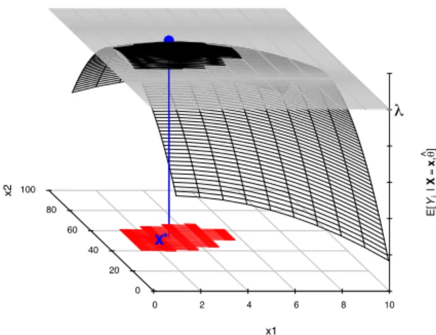
Graphically, the results of such optimization process can be nicely represented if the dimensionality is moderated, as illustrated on Figure 1.2. Notice the data used to create all the graphs hereafter are artificial.
The majority of statistical packages are able to provide such optimization results. However, there is no clue that using the operating condition x∗ will produce a satisfactory output. Indeed, at optimum, the result will be on average better than
Response surface 0 2 4 6 8 10 0 20 40 60 80 100 x1 x2 E[ Yj |X = x, θ ^ ] ● x*
Figure 1.2: Illustration of a response surface model with an optimal solution x∗.
with any other operating condition (in the explored domain χ). But this does not imply a high quality. Also, if the result is subject to noise, caution should be taken regarding the optimum. The analysis of the model parameters and classical tools such as residuals analysis, Q-Q plots, etc. associated with statistics such as R2 or RMSEP, etc. may prevent the analyst to use the (mean) results provided by the model.
When envisaging multiple response optimization, the desirability methodology are appealing to aggregate the various (mean) responses into one index representing the quality of the solution, as proposed by Harrington (1965); Derringer and Suich (1980). More details on this subject are given in Chapter 5.
1.3.2
Sweet Spot
A better answer to assess the quality is to define some specification(s), say Λ =
(Λ1, ..., Λm), for the m responses or CQAs envisaged. In this context, not only the
optimal solution is of interest, but instead the set of operating conditions giving outputs with mean CQAs ˆE[Yj | ˜x] within the specifications Λj. This is the concept
for an univariate problem with one CQA Yj, it is defined as:
Sweet Spot = nx ∈ χ | ˆ˜ E[Yj | ˜x] ∈ Λj
o
,
=nx ∈ χ | f˜ j(˜x; ˆθj) ∈ Λj
o
. (1.1)
It is possible to represent graphically the sweet spot when dimensionality is limited, as shown in Figure 1.3. In this example, the assumed specification Λj is to obtain Yj ≥ λ, i.e. the jth CQA must be higher than a specified value. The zone of the
experimental domain where the mean response surface is higher than λ defines the Sweet Spot (in red). The interpretation is as follows: in this zone, the response is, on average, within specifications. Of course, an optimal solution may still have sense to define exactly the operating condition to use.
Response surface 0 2 4 6 8 10 0 20 40 60 80 100 x1 x2 E[ Yj |X = x, θ ^ ] ● x* ● λ x*
Figure 1.3: Illustration of a univariate Sweet Spot. In red is the subpart of χ providing an expected CQA better than λ (dashed plan).
When considering a multivariate responses process, Sweet Spot methodology is generally used on the overlapping mean response surfaces. The idea is then to find a subpart of χ where every mean response is located within its specifications. This can be written as follows:
Sweet Spot =n x ∈ χ | ˆ˜ E[Y | ˜x] ∈ Λo (1.2) =n x ∈ χ | ˆ˜ y1|x∈ Λ1 \
... \ yˆm|x ∈ Λm
o
,
where ˆE[Y | ˜x] is the multivariate mean response surface and Λ is the set of
The sad news about Sweet Spot is that the provided solution gives limited guar-antees that the quality will be observed in the future use of the method, under the presence of inevitable uncertainties (Peterson, 2009; Peterson and Lief, 2010; Schofield, 2010). Indeed, in the Sweet Spot, considering a symmetric distribution for Yj, and εj being an additive error, the mere interpretation is that there is at
least 50% of chance to observe the univariate response within specification, that is,
P (Yj ≥ λj | ˜x, ˆθj) ≥ 0.5. At the border of the Sweet Spot, there is one chance out
of 2 to be out of specification when dealing with an univariate problem, if the model can be assumed correct.
Finally, correlation structures that might exist between the simultaneous re-sponses are completely ignored, which further increases the risk to take wrong de-cision. As an example, considering two responses Y1 and Y2, assumed independent and predicted at an operating conditions ˜x, situated at the border of each univariate
Sweet Spot, such that P (Y1 ≥ λ1 | ˜x, ˆθ) = 0.5 and P (Y2 ≥ λ2 | ˜x, ˆθ) = 0.5. The
only guarantee about the joint acceptance of both specifications is then, using the rule of product for independent variables, P (Y1 ≥ λ1, Y2 ≥ λ2 | ˜x, ˆθ) = 0.52 = 0.25. In other words, there is 1 − 0.25 = 0.75 probability that the actual outputs are not within both specifications, although the solution lies within the Sweet Spot. If correlations were present and taken into account, this result would be different.
Because the responses/CQAs dependencies are not taken into account, the use of (overlapping) mean responses and Sweet Spot may certainly give unexpected and unexplained results for the future use of the method or process.1
1.4
Design Space
As explained in the previous sections, the basic use of DoE for optimization is generally not sufficient to achieve the risk-based perspective advocated for the QbD approach. The issue comes from the use of mean responses (CQAs) derived from the statistical model. Hereafter are summarized the flaws of mean responses.
Mean responses does not provide sufficient clues about the method re-liability. Assuming a statistical model is appropriate to describe data, the only interpretation of an univariate mean response is that the results are at least as good as the predicted one in about 50% of the runs (i.e., on average). Conversely, one can expect 50% of future results to be not that good ! The obvious solution is to work on
1Notice the examples in the appendix of ICH Q8 (2009) are all about Sweet Spot, which is
believed non compliant with a fully QbD strategy. However, the document states that proven (univariate) acceptable ranges continue to be acceptable from the regulatory perspective but are not considered as a design space (Section 2.4.5 and Question and Answers B.1.Q8.)
the complete distribution of the responses instead of point estimates. Uncertainty and dependencies between responses are the keys to assess reliability. The previous section has also explained the problem when comparing mean responses to minimal specifications.
Mean responses give limited information on the future performance. The purpose of optimizing or validating a method is to give evidences that it will per-form appropriately in its future use, i.e. most of the time, the outcome will meet quality criteria. The use of prediction intervals can be thought as a nice tool for this. Indeed, intervals are practical to express the uncertainty of the responses in a comprehensive way. But unfortunately, they do not quantify the guarantees or risks to be within or outside specifications, respectively. Intervals are then less ap-propriate when envisaging a risk-based approach, even if they integrate the various sources of uncertainty.
1.4.1
Definition
To explain the QbD practice, ICH Q8 guideline defines the important concept of Design Space (DS), central in this manuscript. The DS is “the multidimensional
combination and interaction of input variables (e.g., material attributes) and pro-cess parameters that have been demonstrated to provide assurance of quality”. The
objective of ICH Q8 is to improve the way to understand and gain knowledge about a process or method to find a parametric region of robustness for future performance of this process or method, in order to provide the guarantees of quality. To compute these guarantees, the idea is to replace the expectations in Equations (1.2) with a probability measure to obtain the results within specifications (Chiao and Hamada, 2001). Mathematically, a simplistic but pragmatic DS definition is as follows, for a univariate or a multivariate response:
Design Space =nx ∈ χ | P (Y˜ j ∈ Λj | ˜x, ˆθ) ≥ πj, j = 1, ..., m
o
,
=nx ∈ χ | P (Y ∈ Λ | ˜˜ x, ˆθ) ≥ πo. (1.3) The main differences between Equations (1.2) and (1.3) is that the latter is about an acceptance probability that is compared to a minimal quality level πj (marginally)
or π (jointly). In the frequentist statistical framework, a common solution to ob-tain this probability estimate is to use the assumed distribution of the error εj in
repeated sampling, with the parameters assumed known (Normal distribution) or estimated using the available data (Student’s distribution). Obviously, the joint distribution of the responses must be considered when envisaging the computation of joint probabilities.
Figure 1.4 illustrates the results of such computations. First, Subfigure A depicts an hypothetical univariate distribution of a response Yj for a given x∗, assumed
A 0.0000 0.0005 0.0010 0.0015 0.0020 density of Yj at x* Density Yj values P(Yj>λ )| x*,θ) λ πj =0.9 0.7 0.5 j j ^ B 0 2 4 6 8 10 0.0 0.2 0.4 0.6 0.8 1.0 0 20 40 60 80 100 x1 x2 P( Yj >λ | x, θ) Probability surface ● π x* DS j j ^ C 0 2 4 6 8 10 0.0 0.2 0.4 0.6 0.8 1.0 0 20 40 60 80 100 x1 x2 Probability surface ● ● π x* DS P(Y j >λ | x, θ) j ^ j D 0 2 4 6 8 10 0.0 0.2 0.4 0.6 0.8 1.0 0 20 40 60 80 100 x1 x2 Probability surface ● π x* P(Y j >λ | x, θ) j ^ j
Figure 1.4: (A) Density at optimal condition. Shaded zone: Probability that Yj ≥ λj. (B-C-D) Surface of the probability that Yj ≥ λj for every operating conditions,
and Design Space (in red) at various quality levels. (B) Quality level of πj = 50%.
Similar results than Sweet Spot. (C) Quality level of πj = 70%. (D) Quality level
of πj = 90%, no Design Space is identified.
optimal. On this basis, the proportion of this distribution that is higher than a value λj can be computed (blue). It expresses the guarantee (i.e. the probability)
to observe Y ∈ Λ. In this example, let’s assume we are interested in Yj ≥ λj.
Repeating the operation on every point ˜x ∈ χ, it is then possible to draw a map
of these probabilities, as illustrated on the Subfigures B,C and D. The difference between these three images is the level of πj. On Figure 1.4 (B), the minimal quality
level πj is set to 50% (shaded grey plan), and the operating conditions satisfying
this quality level are said to belong to the Design Space (red) with πj = 50%. As it
could be expected with a symmetrical distribution, choosing πj =50% leads to the