Assessing the Interaction between Real Estate and Equity in
Households Portfolio Choice
Kevin E. Beaubrun-Diant and Tristan-Pierre Maury
yPreliminary version
October 24, 2011
Abstract
In this paper, we provide a new empirical analysis of the dynamic portfolio decisions of households by simultaneously considering their stock market participation and home tenure choices. There is already a huge body of literature on housing status (own/rent) decisions and many contributions doc-umented the low stock market participation rate of US households. Although some papers evidenced that the home status (modeled as an exogenous variable) has an impact on the stock proportion in portfolio, our paper is the …rst one to allow both decisions (home and stock) to be simultaneous and endogenous. We estimate a dynamic bivariate logistic panel data model on Panel Study of income Dynamics data from 1999 to 2007 controlling for sample selection bias and time-invariant unobserved heterogeneity. We …rst evidence that our original joint setup outperforms a standard one (with two distinct equations for stock holdings and for home tenure), i.e. marginal odds ratios are signi…cant. Using these estimates, we are able to simulate individual paths of stock and home equity positions over the life cycle according to households attributes. Ceteris Paribus, we show that households taking positions in one asset (home or stock) encounter a positive position in the other asset at an earlier stage in their life cycle, i.e. some households appear to be locked in a no-stock-and-renter position.
University Paris-Dauphine, LEDA-SDFi. Email: kevin.beaubrun@dauphine.fr.
1
Introduction
Physical real estate accounts for a large share of the wealth of households in many developed countries. In the US, according to the Survey of Consumer Finances (SCF), the owner-occupier rate in 2007 is 68:6 percent and housing represents almost 60 percent of households’total assets. Simultaneously, stocks only accounts for 17:9 percent of the value of total …nancial (i.e. excluding home equity) assets of all US famillies. Many academic contributions tried to provide a theoretical explanation to this so-called stock market participation puzzle (or equivalently the equity premium puzzle): the majority of US households do no participate in the stock market though mean and variance of returns are historically attractive compared to other …nancial assets like bonds, saving bonds, retirement accounts, cash value life insurances, etc. Recently, some papers have put the emphasis on the role played by real estate holdings in explaining household portfolio choices and in particular stock market participation. They rely on the fact that housing is a non standard asset –it is singular with low divisibility (large costs when adjusting the consumption of housing services) and low liquidity (…xed transaction costs and non zero time-to-sell) –whose holding might distort the optimal composition of a household’s portfolio.
Standard models of portfolio choices suggest that a zero position on the stock market cannot be optimal for risk averse agents. In a dynamic empirical contribution, Vissing-Jorgensen (2002) proposed some re…nements compared to the standard setup. She uses two mechanisms: heterogeneity in non…-nancial income patterns and stock market participation costs. Considering a …xed transaction costs may explain why previous non stockholders (i.e. …ve years before in her dynamic setup based on PSID data) have a lower probability to participate in the stock market. Su¢ ciently large costs may dissuade house-holds with low …nancial wealth to enter the stock market. The author also explains how heterogeneity in non…nacial income may help to reproduce the changes in equity shares in households participating in the stock market.
As pointed out by Grossman and Laroque (1990), housing is simultaneously a consumption good and an investment asset, thereby distorting its holdings in household portfolio: the value of home equity is much larger than it should be if housing was a standard …nancial asset. Building on this seminal contribu-tion, Yao and Zhang (2005a) evidence that housing transaction costs might help in explaining households’ stock market participation decisions1. They extend the setup of Cocco (2004) or Hu (2005) which shows
1Some theoretical contributions already simultaneously deal with the determinants of home tenure and equity market
that homeownership crowds out stocks in net worth and incorporate a home tenure owner/renter trade-o¤. Their results suggest that owners hold a higher equity proportion in their liquid …nancial assets (i.e. stocks and bonds) than renters. The authors attribute this fact to the bu¤er role against …nancial risks played by home equity. They also detect that households with low …nancial wealth mainly choose to hold riskless assets (bonds) rather than stocks or real estate because of the …xed costs associated with stock market participation and mortgage down-payment liquidity constraints associated with access to home-ownership. Moreover, the authors provide evidence that households with low home value–net worth ratios and large mortgage–net worth ratios experience large probability to become stockholders. Kullmann and Siegel (2005) also focussed on the role of home tenure in equity holdings in a empirical contribution with panel data. In line with Vissing-Jorgensen (2002), they proposed a dynamic panel data model, hence controlling for possible state dependence in stock market participation. Their main results are similar to those obtained by Yao and Zhang (2005a). They also investigate the relationship between exposure to real estate (i.e. background risk measured by the local volatility of the dwelling value of homeownerss) and shareholding and found a signi…cant role for this factor.
Our article di¤ers from previous studies by explicitly dealing with the potential simultaneity of home tenure and equity market participation choices. In most of the contribution to this literature, the analysis is focused on the impact of home tenure on equity holdings while the reverse is not considered. Home tenure (at least in the empirical literature) is treated as independent from the position in the stock market and even exogenous in some cases. In our opinion, such a hypothesis may be too strong: for example, let us consider the situation of a household currently renting its housing services with low liquid …nancial wealth (small amount of bonds, no stocks). Suppose this household is hit by a large positive non…nancial income shock permitting it either to pay the transaction costs associated with equity market participation or to constitute a su¢ cient downpayment toward becoming owner-occupier. In this case, the joint nature of both decisions is evident: at a certain date, the household must choose between becoming a owner with no stock and becoming a stock market participant while staying in the housing rental sector. Di¤erently said, the problem does not reduce to a choice between two categories fstockholder, non stockholderg for each kind of tenant, but to a choice between four categories fstockholder, non stockholderg fowner, renterg. The potential importance of this simultaneity issue is
signi…cant role in explaining home and stock ownership. As investors become olders, their decisions regarding home tenure and stockholdings are being distorted: this is the hump-shaped life-cycle home and stock ownership pattern. Moreover, the theoretical framework shows that the previous home equity position of household also a¤ects their cross decisions on housing and stock markets over the life-cycle.
also clear when considering the possible wealth reallocation of households at each date. Though most of US households choose to invest in riskless assets to constitute their mortgage downpayment, it appears that a fraction of households participating in the equity market may choose to sell their stocks to get a mortgage loan with eligible Loan to Value ratios and then become homeowners.
To quantitatively assess the importance of joint home-stock decisions, we estimate a bivariate dynamic logit model on data from the Panel Study of Income Dynamics (PSID) from 1999 to 2007 (i.e. 5 waves at a biannual frequency)2. We collect information regarding the home and equity positions of 2163 US households, as well as di¤erent socio-demographic factors (gender, age, marital status, number of children), real income, real net worth (i.e. bonds, stocks and home equity), ratio of mortgage over house value and time dummies.
Our model provides some empirical re…nements about the quantitative importance of joint home-stock decisions of US households and the covariates creating wedges in this simultaneous choices. We estimate an original bivariate dynamic logit model in the line of Bartolucci and Farcomeni (2008). We simultaneously estimate three equations: (i) two marginal conditional logit equations (the …rst one for equity market participation and the second one for home tenure) with state dependence terms (lagged position variables) and unobserved heterogeneity terms to control for household speci…c e¤ects, (ii) a log odds-ratio equation conditional on some selected covariates accounting for potential simultaneity in home and stock market decisions.
We …nd that our original joint setup outperforms a standard one (with two distinct equations to model stock holdings and home tenure), i.e. marginal odds ratios are signi…cant. Our results may be summarized as follows: …rst, contrary to some contributions in the existing literature, we do not …nd that homeownership crowds out stock holdings (…rst logit equation): in line with some previous results within dynamic models, previous owners are more likely to become stockholders. Moreover, the negative impact of home equity on stock market participation decisions already evidenced in the literature with older data (between 1984 and 1999) –the low liquidity of home equity –is no longer signi…cant in our recent sample. The enlarged access to home equity withdrawal in the beginning of the 20000s may have increased the
liquidity of home equity. Second, we …nd a positive contribution of current stock market participation on the probability to be a future owner-occupier (second logit equation). Households with a large share
2We exclude preceeding waves since before 1999, the typical PSID survey frequency was 5 years which might be too long
of equity in …nancial wealth (possibly those with greater risk aversion) are more prone to convert their …nancial wealth into home equity than households mostly holding bonds. Hence, we evidence a two-sided dynamic relationship between home tenure and stock market participation: past home position signi…cantly in‡uences equity market participation and conversely. More precisely, households taking positions in one asset (home or stock) encounter a positive position in the other asset at an earlier stage in their life cycle, i.e. some households appear to be locked in a no-stock-and-renter position. Finally, we …nd that some factors (age, home equity, whether the household holds other real estate assets) have a signi…cant impact on the log of odds ratio (third equation). In particular, it appears that young households have a higher probability to become simultaneously owner and stockholder than older ones, ceteris paribus.
We then extend our setup and add three continuous equations for the determination of the value of stocks, bonds and home equity held by each household. The whole model (three participation equations, three continuous equations) enables us to simulate individual historical paths on the two markets (home and stock) over the considered period and to quantitatively assess the role of the log odds ratio in cross decisions.
The paper is organized as follows: Section 2 presents the econometric methodology. Section 3 describes the dataset. Section 4 presents the whole set of results and the sensitivity analysis. Section 5 concludes.
2
The Econometric Model
2.1
Dynamic Logit Equations
Let yk;i;t denote the categorical response variables for household i at calendar year t, with i = 1; :::; n,
t = 2001, 2003, 2005 or 2007 and k = h; s. yh;i;t is the home tenure and has two categories
{owner-occupier, renter}. ys;i;tis the stock market position and has two categories {stockholder, non stockholder}.
yi;t denote the vector with elements yk;i;t and xi;t is the (1 K) vector of strictly exogenous covariates
for household i at date t. This vector includes socio-economic factors such as age of head (linearly speci…ed), number of adults in household, number of children, log of real household income (two years before), log of real networth (two years before), the log of home equity over value of home (two years
before) and dummies regarding whether the household own a business or another real estate asset than its current home. This vector also contains temporal dummies (for years 2003, 2005 and 2007) to capture the temporal dependence of home tenure and stockholding positions: as previously explained in the data section, the homeownership and stockholders rate are steadily rising over the considered period. Lagged variables yk;i;t 1(i.e. previous year home tenure and stock market position) are included to capture state
dependence, i.e. the direct impact of past positions on current choices. The panel structure of our data sample (we follow the same households for a long period - 6 years - and may then observe multiple spells) permits the identi…cation of an unobserved time-constant heterogeneity term !i.
Let p (yi;t j xi;t; yi;t 1; !i) denote the conditional distribution of the vector of endogenous variables
yi;tgiven the vector of exogenous covariates, lagged endogenous variables and unobserved random terms.
Following Bartolucci and Farcomeni (2008), we adopt a local speci…cation for marginal logits and for log-odds ratios. More precisely, each of the two marginal logits k;i;t is modeled as follows
k;i;t= log
p (yk;i;t= 1 j xi;t; yi;t 1; !i)
p (yk;i;t= 0 j xi;t; yi;t 1; !i)
k = h; s (1)
where the value taken by yk;i;t determines the home tenure (k = h) or the stock market position (k = s).
In the former case, we arbitrarily select the category yh;i;t= 0 to denote the renter state while yk;i;t= 1
is for homeownership. In the latter case, ys;i;t = 0 is for non-stockholder position and ys;i;t = 1 for
stockholders.
The marginal log odds ratio 'i;t is speci…ed as follows 'i;t= log p (yh;i;t= 1; ys;i;t= 1 j xit; yit 1; !i)
p (yh;i;t= 0; ys;i;t= 1 j xit; yit 1; !i)
p (yh;i;t= 0; ys;i;t = 0 j xit; yit 1; !i)
p (yh;i;t= 1; ys;i;t = 0 j xit; yit 1; !i)
(2) This log odds ratio measure the gap between the pair of conditional logits. For example, a large value for 'i;t (i.e. a log odds ratio largely positive) means that the ratio of probability of being an
owner-occupier (yh;i;t = 1) compared to a tenant in the private rental sector (yh;i;t = 0) for household
i at calendar year t is higher when holding stocks (ys;i;t = 1) rather than not (yh;i;t = 0). Hence,
the value taken by 'i;t is extremely important for the purpose of this paper: if it strongly diverges from zero, it necessarily means that current decisions of household on one market (the stock market for example) are related to current – i.e. not solely past positions – choices on the other market (home tenure). Di¤erently said, it would mean that household’s decisions regarding their home tenure and stock
market participation are simultaneously rather than sequentially taken in their life-cycle. We propose the following simple three-equations linear setup for marginal logits and log odds ratio
8 > < > :
k;i;t = k+ xi;t k+ yi;t 1 k+ !k;i; k = h; s
'i;t= + xi;t + yi;t 1 + !i;
(3)
k (resp. ) are the intercept terms for each marginal logit equation (resp. log odds ratio). The
unobserved heterogeneity factors !i (k = h; s) and !i are elements of vector !i. As will be detailed in
the next subsection, !i also includes terms from the di¤erent continuous equations that we will have
to estimate to conduct the model simulation. The vector of covariates xi;t in the log odds equation
only include a fraction of the elements of vector xi;t: we have to be parcimonious when modelling odds
ratios in order to limit the number of parameters to estimate3. Notice that supposing that some factors
a¤ecting the marginal logits do not impact the log odds ratio is equivalent to assuming that the underlying utility function of households is separable in these factors: the contribution of this variable to the current endogenous household’s decision on one market (home tenure for example) does not distort the current endogenous decision on the other market (stock market in this case). k;z (resp. ) is the (K 1) vector of parameters that evaluates the impact of exogenous covariates of marginal logits (respectively log odds ratio). k (resp. ) is the vector of parameters assessing the contribution of last year home tenure and stock market position on current marginal logits (resp. log odds ratio).
Overall, the simultaneous estimation of the two marginal logits k;i;t and the only log-odds ratio 'i;t delivers a complete characterization of the joint conditional distribution of ys;i;t and yh;i;t. Once the
three corresponding equations have been estimated, we use the approximate iterative procedure described by Colombi and Forcina (2001) to obtain p (yi;t j xi;t; yi;t 1; !i) from the vector h;i;t; s;i;t; 'i;t . This
procedure4 is computationally cumbersome since it requires an optimization process within our likelihood
maximization procedure. This explains that we have to keep the number of parameters reasonably low.
2.2
Continuous equations
In a …rst step, we will limit our analysis to stock market participation and home tenure decisions. The results of the estimation of the three-equations system (3) is largely detailed in the …rst part of the results
3For example, Bartolucci and Farcomeni (2008) treat the log odds ratio as constant. 4We use MATLAB functions made available by Bartolucci (2007).
section. However, we will further need to complete our setup with three continuous equations for the determination of the amount of shares, home equity and bonds held by each household, since the lag of these variables enter the dynamic logit equations (vector xi;t) and are a¤ected by current home tenure
and stock market participation choices of this household. More precisely, for the simulation of the model, we need to estimate (i) the amount of shares si;t among stockholders since the value of si;thas an impact
on the composition of the household real networth which is a component of xi;t and will then impact
future home tenure and stock market participation decisions, (ii) the value of current home equity heit
among homeowners (which will also a¤ect future transitions of households) and (iii) the value of real non-stock liquid …nancial wealth bi;t.
We then estimate a three-equations system with continuous endogenous variables. Among the explanatory variables, we include almost all those already present in vector xit as well as additional
factors usually present in this kind of model: lagged values of the log of all three endogenous variables:
si;t 1, heit 1 and bi;t 1 for previous (i.e. two years ago) stockholders, homeowners or bondholders as
well as three dummies (ds;i;t 1, dh;i;t 1 and db;i;t 1) taking the value 1 for non-stockholders, renters,
non-bondholders respectively and zero otherwise. The system is as follows 8 > > > > > < > > > > > : log si;t
nwi;t = s+ [xi;t; zi;t] s+ yi;t 1 s+ !s;i+ "s;i;t
log (hei;t) = h+ [xi;t; zi;t] h+ yi;t 1 h+ !h;i+ "h;i;t
log (bi;t) = b+ [xi;t; zi;t] b+ yi;t 1 b+ !b;i+ "b;i;t
(4)
The interpretation of parameters s, s, h, h, b, b is straightforward following the presentation of
system (3). The vector zi;tcontains all additional covariates compared to those included in the transition
equations. We also include three vectors of parameters s, h and b since the previous stock market
position or home tenure (owner or private renter) may impact the composition of the real networth nwi;t.
!s;i, !h;i and !b;i are unobserved time-constant heterogeneity terms, possibly correlated with those
included in system (3). The potential link between these three terms is essential since it may capture wealth reallocation e¤ects (i.e. households converting non …nancial into …nancial assets for example). "i;t = f"s;i;t; "h;i;t; "w;i;tg is a supposedly homoskedastic Gaussian error term vector5, "i;t N (0; ).
Let g1(sitj xi;t; zi;t; yi;t 1; !s;i) be the density of stock values conditional of observed and non observed
factors. Let g2(heitj xi;t; zi;t; yi;t 1; !h;i) and g3(bitj xi;t; zi;t; yi;t 1; !b;i) denote the equivalent density
5 could also contains non-zero diagonal elements to reproduce time-dependent reallocation e¤ects not captured by
functions for home equity and bond values of household i at date t respectively.
2.3
Unobserved heterogeneity
The joint distribution of the six (two marginal logits, the log odds ratio and three continuous equations) heterogeneity terms of vector !i= f!s;i; !h;i; !i; !s;i; !h;i; !b;ig is assumed to be normal !i N (0; ) :
is supposed to be time homogenous. We have to estimate six variance terms (included in vector 2 !) and
15 linear correlation terms6 (vector !).
2.4
Likelihood inference
Let Li;t(!i) be the likelihood expression for household i at date t conditional on all strictly exogenous
covariates (omitted from the argument of likelihood to keep notations simple), on past stock market positions and home tenure of the household (also omitted) and on heterogeneity terms !i. The expression
for log-likelihood is
Li;t(!i) = p (yi;t j xi;t; yi;t 1; !i) [g1(sitj xi;t; zi;t; yi;t 1; !s;i)]es;i;t (5)
[g2(heitj xi;t; zi;t; yi;t 1; !h;i)]eh;i;t[g3(bit j xi;t; zi;t; yi;t 1; !b;i)]eb;i;t
with es;i;t = 1 if household i participates in the stock market at calendar year t and zero otherwise.
eh;i;t = 1 if household i is an owner-occupier at date t and zero otherwise. eb;i;t = 1 if household i
holds bonds at date t and zero otherwise. We deduce the overall expression of the joint non conditional log-likelihood L = N X i=1 log (Z p (yi;1999 j !i) " 2007 Y t=2001 Li;t(!i) # dF (!i) ) (6) where F (:) is the cumulative normal distribution function of unobserved heterogeneity terms with variance-covariance matrix . The term p (yi;1999j !i) is included because of the initial condition
prob-lem: the …rst lag of endogenous variables yi;1999is possibly correlated with the unobserved time-constant
heterogeneity factor. The complete model of transitions on housing and labor market, wages and housing costs is estimated with maximum likelihood techniques with a large number (i.e., 15) of simulated values for each component of vector !i.
6An alternative modelling procedure proposed by Heckman and Singer (1984) where ! is a discrete random vector with
3
Data
3.1
Data description
For the seek of our study with state dependence e¤ects, we rely on panel datasets. As we mainly focus on the di¤erent asset classes (stocks, bonds, bank account savings, current accounts) held by U.S. households, we choose to use the Panel Survey of Income Dynamics (PSID hereafter). The Family …les data are collected over the [1999 2007] period. This sample period choice is …rst motivated by the fact that the Wealth Supplement surveys are useful to reconstitute households’ …nancial wealth and home equity are also available for those years. Moreover, starting from 1999, the survey frequency is two years (compared to …ve years before 1999): such a frequency reduces the risk of unobserved spells (more than one transition between two interviews): this point is extremely important since we focus on transition rates to homeownership and stock market participation. Unobserved spells would conduct to biased transition rates. Following Vissing-Jorgensen (2002), we exclude the Poverty and the Latino Sample. As detailed in the literature, lower and upper centiles for each interest variables are deleted to control for possible outliers7.We only keep those families whose structure has remained unchanged throughout the period of
observation to limit the possible impact of socio-demographic choices on our interest variables. Moreover, our …nal dataset only contains informations for each of the households ever in the sample throughout the [1999 2007] period (Vissing-Jorgensen, 2002 or some of the results of Kullmann and Siegel). This – quite standard –assumption is necessary in our dynamic setup since one missing observation for a given household at a certain date conducts to two missing points for the estimation because of state dependence terms.
We collect informations from the two following PSID datasets: the …rst group of variables comes from the Family …les8. These variables are used to characterize the surveyed household: age of head,
number of household’s members, number of children, residence location code. We also retain a measure of households’income and the situation of the household on the housing market (renter or owner) and the value of the property for owner households. Finally, we retain the amount of the principal and secondary mortgages for homeowners.
The second group of variables is collected in the Wealth Supplement, which precisely describes the
7With this procedure, most of the top-coded variables (for wealth or income for example) are suppressed.
8We use family instead of individual …les since the latter do not contain wealth informations. We nevertheless have to
components of wealth held by American households. We retain a de…nition of total wealth including home equity. The households’wealth is calculated by summing the following types of asset: if own part or all of a farm or business, money in checking or savings accounts, money market funds, certi…cates of deposit, government savings bonds or treasury bills not including assets held in employer-based pensions or IRA’s, any real estate other than a main home9, shares of stock in publicly held corporations, mutual funds or
investment trusts10, other physical assets11, other savings or assets12. The …nancial wealth variable is the sum of cash, bonds and stocks and is net of the value of debt. This latter variable is de…ned as other debts aside from any mortgage or vehicle loans, such as credit card charges, student loans, medical or legal bills, or loans. The sum of …nancial wealth and home equity is total wealth.
Since we seek to explain the joint decision of housing tenure and participation in the stock market (hold shares/shares not held), the dependent variables are OW N HOU SEitet OW N ST OCKit. Notice
that the lag of these variables (i.e. the home tenure and stockholding position at the preceding interview, two years before) will be included among the set of explanatory variables. The covariates are the following: RN ET W ORT Hit measures the total real net wealth13 of a given household i at period t. The
variable, RIN COM Eit, measures the total family income collected in a given year14. As this variable
can contain either null or negative values (which indicates a net loss), we exclude such observations and only keep households with non-negative income.
ST OCKitrepresents the value of shares held by households in the sample. This variable includes
shares of stocks in publicly held corporations, mutual funds, or investment trusts, not including stocks in employer-based pensions or IRA’s.
LH_EQit, is the logarithm of the home equity de‡ated by the Consumer Price Index. The value
of home equity is built with the house price P Hitand the outstanding primary plus secondary mortgage
value M ORT GAGEit. P Hit is de…ned as the current value of the apartment or house self-assessed by
the household. The value M ORT GAGEittaken by this variable represents the principal currently owed
9Such as a second home, land, rental real estate, or money owed on a land contract 1 0Not including stocks in employer-based pensions or IRA’s
1 1Cars, trucks, motor home, trailers or boats.
1 2Such as bond funds, cash value in a life insurance policy, a valuable collection for investment purposes, or rights in a
trust, money in private annuities or Individual Retirement Accounts (IRAs)
1 3We depart from the nominal (W EALT H
it)given in the Wealth Supplement and use the Consumer Price Index variation
between the considered year and 1984, FRED (Federal Reserve Economic Data) Economic Research Division Federal Reserve Bank of St. Louis CPIAUCSL.xls; Consumer Price Index for All Urban Consumers: All Items; Index 1982-84=100; M; SA; 2010-12-15. http://research.stlouisfed.org/fred2/categories/9
1 4For each year, the total family income is the sum of these seven variables: Head and Wife/"Wife" Taxable Income,
Head and Wife/"Wife" Transfer Income, Taxable Income of Other FU Members, Transfer Income of OFUMS, Head Social Security Income, Wife/"Wife" Social Security Income, OFUM Social Security Income.
from all mortgages or land contracts on the home. The ratio (M ORT GAGEit=P Hit), de…nes the share
of mortgages with respect to the value of the house. It measures the degree of household home leverage. W BU SINit, W OREALit are binary variables (= 1 when the household owns part or all of a farm
or business or when anyone in the family owns any real estate other than the main home, i.e. a second home, land, real estate for rental purpose). For these variables, we allow the business assets, and other types of asset holdings to in‡uence the decision to buy a home or to enter the stock market.
y2003, y2005, y2007 are dummy variables that account for the business cycle impact on the decision to buy a home or to participate in the stock market. Year 2001 is the reference. The remaining explanatory variables are AGEit, N U M KIDSit, N BADU LT Sit, which respectively denote the age of head, the
number of kids and adults. This latter variable is obtained by subtracting the number of kids from the total number of household’s members. All these variables are linearly speci…ed.
Conditionally to the …rst double decision related to the participation equations, we will also need to determine the share of household’s net wealth invested in di¤erent types of assets: bonds bit, stocks sit
and home equity. The determination of these continuous variables is necessary for the simulation of the model. The vector of dependent variables is : sit=nwitthe proportion of shares of stocks in the networth
of the household, LH_EQit, the logarithm of home equity and log (bit) the logarithm of the bond and
other risk-free assets value.
3.2
Summary Statistics
We now provide some descriptive statistics for di¤erent subsamples of households for our sample period [1999 2007]. We focus on key identical variables across di¤erent subgroups. These variables include the percentage of stock ownership, the fraction of homeowners, the house value-networth ratio, the households’income and networth (in 1984 dollars), the shares to networth ratio, the shares to …nancial assets ratio, the networth to income ratio, the number of children under 18 living in the household, the number of adults in the household, the percentage of households owning a business and the percentage of households owning other types of real estate assets.
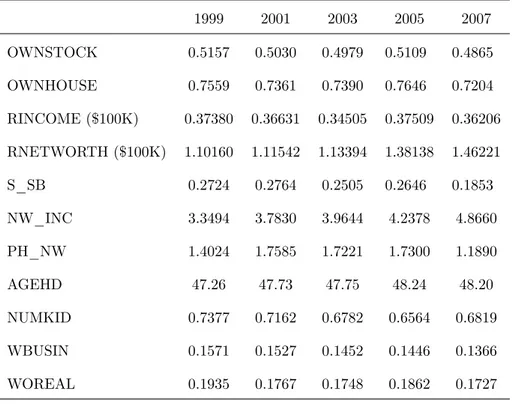
Table 1 illustrates the year by year evolution of the variables of interest. We …rst observe that the average age of head slightly increases from 47.2 to 48.2 years over the [1999 2007] period. The number of children per household is about 0.73 in 1999 and steadily diminishes to 0.68 in 2007. The share of
households with other real estate assets remains steady over the observation period (between 17:2 and 19:3%). Similarly, the proportion of households owning a business is relatively constant over time, in spite of a fall in 2007.
When it comes to explain the stock market participation, we observe that the share of shareholders is around 50%. Despite a slight recovery in 2005 (51:9%), the trend is clearly negative slopped between 1999 and 2007 (48:6% in 2007). We detect a similar evolution for the homeownership trend: 75:5% of the households were homeowner in 1999 against 72% in 2007. Regarding the composition of the portfolio (…nancial and real estate) held by the average household and its evolution over the [1999 2007] period, we learn from Table 1 that the proportion of shares in liquid …nancial wealth of households, in 1999 was worth 27:2% but only 18:5% in 2007.
With these elements in hands, we are able to highlight some sharp contrasts between renters and homeowners. Table 2 shows that the percentage of households participating in the stock market is higher for homeowners than for renters. Homeowners are on average more likely to participate in the stock market. For example, in 1999, 58:5% of homeowners were shareholders against 30% in the renters’ population. This proportion slightly increased for owners (59:1% in 2007), while it decreased to 21:6% in 2007 for renters. Moreover, the amount of shares relative to the …nancial (liquid) networth of homeowners is twice as high as of renters. This gap widens along the sample period. In their contributions, Kullmann and Siegel (2005), Yao and Zhang (2005a) and Vissing-Jorgenssen (2002) evidenced similar patterns. Another point highlights the contrast between homeowners and renters: despite a higher rate of stock market participation of the owners, their risk exposure is much lower. Indeed, the share of equity shares in net wealth is lower for owners than for renters. This is the traditional "crowding-out e¤ect" detailed by Cocco (2004). Focusing on the role of housing consumption in explaining the cross-sectional heterogeneity of investors’ portfolio decisions, he found that the housing asset crowds out stockholding in net worth. As our sample covers a more recent period than the above contributions, it seems interesting to notice the persistence of these structural di¤erences.
4
Results
This section presents the quantitative results. It is divided into two parts. In a …rst subsection, we present the estimation results. At this stage, we seek to judge the goodness of …t statistics provided
by the econometric model. In a second subsection we present three counterfactual exercises based on simulations. Our goal in simulating these scenarios is to assess the additional information provided by our econometric model on the joint choice to enter the stock market and become homeowner.
4.1
Estimates
We …rst present the parameter estimates of a reduced version of the model, i.e. the system of tran-sition equations (3). Results are summarized in Table 3. Continuous equations will later be added in the simulation subsection. In Table 6, the …rst column lists exogenous covariates, lagged endoge-nous variables and the estimated variances of unobserved terms. The second column gives parame-ters estimates corresponding to the …rst logit equation, i.e. the relative probability of being owner in t compared to renter conditional on past position, exogenous variables and household speci…c terms, p (yh;i;t= 1 j t) =p (yh;i;t= 0 j t) with t = fxit; yit 1; !ig. The third column gives parameter
estimates corresponding to the relative conditional probability of being stockholder rather than not p (ys;i;t = 1j t) =p (ys;i;t = 0 j t). The last column gives estimates corresponding to the log odds ratio
'i;t. The symbol , , means signi…cant at 5% level and at the 10% level. All the reported standard er-rors are heteroskedasticity-robust. Notice that the chosen …nal setup results from previous estimations of enlarged models with many other covariates. Some of them have been discarded with usual log likelihood ratio tests. As previously explained, we only consider households with four consecutive observations (in 2001, 2003, 2005 and 2007). The total number of such households is 2; 163 after dataset treatment, hence the total number of observations is 8; 652. Most of the explanatory variables are lagged to prevent from simultaneity issues: for example, decisions regarding whether to hold another business W BU SINit or
real estate asset W OREALitand those concerning yh;i;tor ys;i;t might be jointly taken; we then have to
lag these variables as well as all the …nancial or economic ones. The only contemporaneous variables are the socio-demographic ones: age of head, number of adults or number of children. We have reduced the number of estimated parameters in the log odds ratio equation: many explanatory variables have been discarded since we detect no signi…cant impact on 'i;t when estimating enlarged setups.
We …rst check for the goodness-of-…t of our model with standard pseudo R2 …t statistics (i.e. log
likelihood ratios comparisons between pairs of models). We …nd that the presence of explanatory variables contributes to improve the likelihood of our model by 36% compared to a very simple model with only intercept terms. The log likelihood discrepancy between our benchmark model and a model with only
the two marginal logit equations (1) but no odds ratio (i.e. setting 'i;t to zero) is above 5%: Hence,
this advocates for the presence of simultaneity e¤ects through equation (2). Moreover, had we deleted cross state-dependence terms, the likelihood gap would have widen to almost 15%: This con…rms the importance of dynamics terms (impact of lagged home tenure on stockholding and of lagged stock market position of home tenure decisions). Finally, we detect a signi…cant role for the unobserved heterogeneity variance terms; but no correlation between the term in the home tenure logit equation and the term in the stock market participation logit equation.
4.1.1 No age e¤ect on home tenure, but a positive in‡uence on stock market participation We found no signi…cant e¤ect of age of head (linearly speci…ed) on the marginal probability ratios of becoming an owner rather than a renter, p(yh;i;t=1j t)
p(yh;i;t=0j t). In a …rst glance, this result seems to stand in
sharp contrast with previous estimates: the homeownership rate grows with age of head, at least before retirement. Our descriptive statistics also con…rms this pattern, but recall that our setup is not focused on the level of stock market participation or home tenure rates, but on the transition rates to homeownership and stockholding. Hence, we detect no signi…cant distortion of transition rates to ownership over the life-cycle, once controlling for other factors such as income or wealth e¤ects. Moreover, we also tested for the role of AGE2
it since, as explained by Yao and Zhang (2005b), the home-ownership rate exhibits
a hump shaped pattern over the life-cycle in the US (with a peak just before retirement). However, we detect no signi…cant contribution for this variable.
On the contrary, age appears to positively in‡uence the transition rate to equity market partic-ipation. Once again, quadratic terms in age have been discarded: our estimates suggest than when controlling for other factors such as income, wealth or previous position (home tenure or stock market participation), the well documented hump-shaped pattern in stock ownership is no longer valid (notice that Kullmann and Siegel, 2005, also fails to detect a signi…cant impact of the square of age of head on stock market participation). This result (i.e., age positively in‡uences stock ownership) is in line with previous empirical studies (for example, Yao and Zhang, 2005a, found a positive in‡uence of age on stock market participation for homeowners): young households with low …nancial wealth and generally no home equity preferentially invest in riskless assets such as bonds. Consequently, their equity share in …nancial wealth is low. Interestingly, we …nd a signi…cant negative contribution of age to the log odds ratio 'i;t: conditionally on past positions on both markets, elderly households exiting to participation in
one market (i.e. either becoming owner-occupiers or stockholders) encounter a lower probability to switch to participation in the other market than younger ones. Di¤erently said, if we compare two otherwise similar households at di¤erent stages in their life-cycle and suppose both are renter and non-stockholders, the younger one experiences a higher probability to become simultaneously owner and stock market par-ticipant at a two years horizon than the older one (when controlling for other socio-economic and …nancial factors). This fact will be clearly illustrated in the simulation subsection. Notice also that head’s age will appears to be one of the few variables signi…cantly contributing to the log of odds ratio (many other potential covariates have been discarded based on log likelihood ratio tests), but this in‡uence is non negligible: if we had solely estimated the two marginal logits equations p(yh;i;t=1j t)
p(yh;i;t=0j t) and
p(ys;i;t=1j t) p(ys;i;t=0j t),
the pseudo R2 …t statistics would have been only 30% instead of 36% for the benchmark.
4.1.2 The role of other socio-economic factors
The number of adults has a positive impact on the ownership transition rate (married heads more fre-quently exit to owner-occupier state than single). Oppositely, this variable negatively in‡uences the probability of participation to the stock market.
Surprisingly, the number of kids living in the household does not play any signi…cant role on stock market participation (this result con…rms Yao and Zhang, 2005a or Kullmann and Siegel 2005 estimates), but nor does it on the transition rate to homeownership. This result could be linked to the possible correlation between this variable and the age of head. As was to be expected, the lagged real income RIN COM Eit 1and the lagged real net worth RN ET W ORT Hit 1 positively in‡uence the conditional
probabilities to become homeowner and stockholder. Concerning the equity market participation, this result is in line with Yao and Zhang (2005a) or Kullmann and Siegel (2005). These results respectively con…rm the role of (non…nancial) income exempli…ed by Vissing-Jorgensen (2002) in explaining part of the cross-sectional heterogeneity in asset holdings and the presence of participation costs (liquidity constraints) on the stock market. Households with low …nancial wealth and home equity cannot pay these entry costs and keep a large share of their wealth in the form of riskless assets. A similar reasoning may be applied to the transition rate to homeownership: households with a low …nancial wealth are not able to constitute the necessary downpayment for a mortgage loan.
4.1.3 The e¤ect of home equity
The log of lagged real home equity LH_EQit 1 has no signi…cant impact on marginal logits though the
signs of parameter estimates are in line with the literature: positive for transition rate to homeownership (previous owner-occupiers with large home equity are more likely to remain owner than those with small home equity), negative for transition rate to stock market participation: Yao and Zhang 2005a, 2005b and Kullmann and Siegel, 2005, found a signi…cant negative contribution of the home value-networth ratio P Hit=RN ET W ORT Hitand a positive of the mortgage-networth ratio M ORT GAGEit=RN ET W ORT Hit
to equity market participation. Hence, their results suggest an overall negative impact of home equity on stock market participation: this is due to the low availability of liquid wealth to pay stock market participation costs for households with a large (rather illiquid) value of home equity. In our case, we do not separately consider the contribution of P Hit and M ORT GAGEit due to a lack of signi…cance,
we only consider home equity as a single covariate. The non signi…cance of the log of home equity on stock market participation in our sample may re‡ect the larger use of home equity withdrawal in the considered period [1999 2007] compared to the sample period of the existing literature (typically the 80’s and 90’s): home liquidation costs and re…nancing charges have decreased and home equity became more liquid recently.
Notice that even though the total real networth does not appear to distort cross-decisions of households on both market (no e¤ect of RN ET W ORT Hit 1 on 'i;t), the composition of this networth
has a signi…cant impact on the log odds ratio 'i;t. For given amount of wealth (i.e. controlling for RN ET W ORT Hit 1), the larger the home equity LH_EQit, the higher the joint probability to be
(more precisely to remain) homeowner and stockholder conditionally on previous states. This suggests that owner with a large home equity over net worth ratio are more frequently simultaneously owner and stockholders at a two years horizon than renters or owners with low home equity. This result is close to what has been evidenced by Yao and Zhang (2005a): home equity acts as a bu¤er against …nancial risk. A fraction of households with low home equity may have to sell their house to participate in the equity market (participation costs hypothesis). They hence have a lower probability to become simultaneously owner and stockholder than households with a large home equity. All in all, our results show that the role of the low liquidity of home equity in our sample period has been reduced compared to previous studies with older sample periods.
participation. First, lagged position on the equity market impacts (at the 10% level) current home tenure choices. Previous stockholders more frequently exit to ownership. Hence, the composition of …nancial wealth (i.e. the ratio of shares to …nancial wealth) in‡uences the transition rate to homeownership. Households may use some of their risky assets to constitute the down-payment for a mortgage loan: ceteris paribus, households with low risk aversion (higher share of equity) may be more prone to convert some of their liquid asset into home equity. Moreover, we also …nd that previous home tenure has an impact on the transition rate to equity market participation. Households currently owning their primary residence have a higher future probability to participate in the stock market than renters. This result somewhat contradicts the well-known crowding out e¤ect of ownership on equity holdings (Yao and Zhang, 2005a), but the latter was obtained in a non dynamic setup (i.e. no state dependence e¤ects). On the contrary, our …ndings are similar to those of Kullmann and Siegel (2005) evidenced in a dynamic panel setup. Overall, households having a positive position in one asset (either being homeowner or stockholder) encounter a higher probability to hold the other asset in the next two years. Di¤erently said, some households appear to be locked in a no-stock-and-renter position.
We do not detect any signi…cant contribution of W BU SINit 1or W OREALit 1. Yao and Zhang
(2005a) found that these two variables negatively in‡uence the transition rate to equity market participa-tion of owners, but these results were obtained with a di¤erent sample period. Finally, we do not detect any cycle e¤ects in transition rates (dummies y2003, y2005, y2007 are rejected –y2001 is the reference).
4.2
Sensitivity analysis
Since our chosen sample period [1999-2007] is di¤erent from the one generally considered in the literature, we have to conduct a sensitivity analysis to disentangle facts resulting from our modelling from those resulting from our speci…c sample period. As previously explained, the [1999-2007] period present some advantages for our analysis: the survey frequency is only two years and it is characterized by a rather steady growth of home prices. However, stock prices have encountered very large movements in the beginning of the 2000’s and we cannot be sure that the presence of time dummies y2003, y2005, y2007 in our setup is enough to control for these dynamic e¤ects. Some structural time-dependence in parameters might still be present.
Consequently, we reproduce our estimation exercise on the [1984-1999] sample period to check for the structural stability of our main results. We collect four PSID waves corresponding to years
1984, 1989, 1994 and 1999. Treatments of the dataset are perfectly similar to those presented in the data description subsection. Once again, we only consider households with four consecutive observations and with no change in structure throughout the period. Compared to Table 6, our set of covariates is slightly di¤erent: we do not directly estimate the impact of LH_EQit, the logarithm of home equity, but
rather di¤erentiate the contribution of the home value (for owner-occupiers) P Hitand of the outstanding
mortgage M ORT GAGEitas done by Yao and Zhang (2005a). We check for the impact of these two terms
on the two marginal logits, but also on the simultaneous log-odds ratio. Notice that we also tested for the in‡uence of squared terms such as (RIN COM Eit)2, (RN ET W ORT Hit)2, (P Hit)2or (M ORT GAGEit)2
but fail to detect any signi…cant contribution. Finally, notice that we do not consider all covariates introduced by Kullmann and Siegel (2003) such as gender, health condition or educational attainment of head to keep the estimation process computationally tractable. However most of the socio-demographic variables are time-constant and are then potentially captured by our unobserved heterogeneity terms, though not directly identi…ed.
Results of this supplementary analysis are available upon request. The main results are similar to our benchmark. We nevertheless detect a signi…cant gap (in absolute value) between the contribution of previous home value P Hitand mortgage M ORT GAGEit of the transition rate to stock market
par-ticipation. This is in line with Yao and Zhang (2005a) and con…rms that the role of these varaibles has changed over time. Moreover, dummies W BU SINit and W OREALit now have a signi…cant impact in
the stock market participation equation. We still do not detect any time e¤ect through y1994 or y1999 time dummies (y1989 is the reference).
Interestingly, our two main results are preserved : (i) the cross-dynamic terms are still signi…cant, OW N HOU SEit 1 positively impacts the transition rate to stock market participation (in line with
Kullmann and Siegel, 2003) and OW N ST OCKit 1 positively impacts the transition rate to
homeown-ership. This con…rms that stock market and homeownership decisions should be jointly modeled: over the life-cycle, some households taking a positive position on one market encounter will participate in the other market sooner than those who did not; (ii) we still detect simultaneous e¤ects: as evidenced in the benchmark model, age distorts the decision to become simultaneously owner and shareholder. Moreover, M ORT GAGEit 1 and P Hit 1 also in‡uence this joint decision. The larger the home value, the higher
the probability to simultaneously participate in the stock market and remain homeowner. The outstand-ing mortgage intuitively has the opposite role. Notice …nally that log likelihood ratios tests suggest that
this speci…cation (with both M ORT GAGEit 1 and P Hit 1) is to be preferred to the benchmark (with
only LH_EQit 1) for the [1984-1999] period.
4.3
Simulation
4.3.1 Methodology
We now use the estimated model to simulate some counterfactual exercises. We select all household’s head for a speci…c year (i.e., the starting year 1999) and simulate their housing tenure, stock market participation and total networth (shares, bonds and home equity) until year 2007. We can then estimate the evolution of the homeownership and stock market participation rates at di¤erent horizons over time. Moreover, with such a setup, we can compare time paths on housing and stock markets of two households with similar pro…le (for example the same socio-demographic characteristics), except in one dimension (for example the family income or the home tenure or stock market participation). We will be able to assess the contribution of this sole factor on future home and stock transition decisions.
The simulation of the role of a household’s characteristics involves several technical steps. First, we select the concerned factor: for example, suppose we want to compare future choices of an owner-occupier household h1 and a household living in the rental sector h2, ceteris paribus. We then select the average
socio-demographic pro…le from our 1999 sample of households and impute it to h1 and h2 (i.e. average
age, number of children, networth and income). We suppose both households do not participate in stock markets in 1999 and that h1 is a homeowner with average home equity) and h2lives in the rental sector
(no home equity, but a similar amount of bonds since we assume the same networth for both households). We simulate home tenure and stock market participation of the two households from 2001 to 2007. We simulate values for shares, home equity and bonds using system (4) each time the households participate in these markets. All other components of vector xi;t and zi;t are kept constant over time
(no change in socio-demographic pro…le) except the log of real income which is assumed to exogenously follow the time pattern of its observed counterpart in the sample.
Overall, for each household, we simulate 2:000 paths on both markets between 2001 and 2007. For each path, we draw a new vector of unobserved factors!biwith our estimates b of the variance-covariance
matrix. The estimates of transition probabilities p (yb i;t j xi;t; yi;t 1;!bi) is evaluated with Colombi and
holdings, a new value for shares, home equity or bonds is randomly drawn using variances estimates b. We …nally compare the transition rates of both households at di¤erent time horizons.
4.3.2 Counterfactual results
The implementation of counterfactual simulations is done with the complete model, i.e. systems (3) and (4). Indeed the simulation of bond, stocks and home equity are necessary to simulate the dynamics of the log of real networth which enters the set of exogenous covariates in the transition equations. Our aim is to measure the e¤ect of a single characteristic. When computing transition probabilities in a given sample, such probabilities are in‡uenced by a variety of factors related to the heterogeneity of agents in that sample. The contribution of these di¤erent factors to determine measured probability is combined and hard to disentangle using only model estimates. However, when simulating our model, it becomes possible to isolate the contribution of a given factor to determine its role on transition probabilities and compare historical paths on both markets.
We propose three counterfactual exercises that aim to investigate the contribution of age, initial position on the housing market and the initial position on the stock market to transition rates. We de…ne an arti…cial household that shares the average 1999 sample characteristics. Its pro…le is as follows: the adult of reference of this household is 49 years old, it is composed of two adults and one child. The average income equals 36; 316 US dollars per year and its networth stands at 32; 533 US dollars. This benchmark household is renter and does not participate in the stock market in 1999.
By age We de…ne three other arti…cial individuals that di¤er from the previously presented one only by age. The …rst one is 69 years old, the second one is 39 years old and the youngest, is 29. The objective of this exercise is to assess quantitatively the impact of age on the choices of home tenure and stock holdings of agents at di¤erent temporal horizons (i.e., 2001 means two years’ horizon and 2007 eight years’ horizon) when controlling for all other factors (in particular all are renters and non-stockholders with similar income and wealth). Table 4 summarizes the results for each type of head’s age at di¤erent time horizons.
At a two-year horizon, we …nd that the elderly have a higher probability to participate in the …nancial market (this is linked to the positive impact of age of head on the marginal logit for stock market participation) than young households. Elderly households have no signi…cantly di¤erent probability
of becoming homeowner than young ones, but a lower probability of being simultaneously owner and shareholder. This result is linked to the impact of age on the log odds ratio 'i;t and con…rms that the simultaneous choice criteria of home tenure and equity market participation are dependent on head’s age. This might illustrate di¤erences in risk aversion according to age. The paradox is raised if one compares the degree of liquidity of both assets (…nancial and real estate). If old agents are more risk adverse (particularly if we consider negative comovements between stock returns and consumption), they also have a higher preference for liquidity. Indeed, though risky, shares remain more liquid than real estate assets: for a given level of wealth, young households might be less sensitive to the low liquidity of housing compared to households close to retirement: for an elderly household renting its dwelling, transition to homeownership may entail the contraction of a mortgage and the imminent prospect nearing retirement – and the loss of income it entails – is a incentive to avoid borrowing, therefore fosters the demand for shares, but lowers the simultaneous demand for shares and housing.
When time horizons get longer, for example at a eight-year horizon, the older household progres-sively has a higher probability of being simultaneously owner and shareholder. We interpret this result as a sign of the impact of the age of head on the relative probability to become stockholder (second column of Table 3): once participating in the stock market, the older household has a higher probability to become homeowner through the positive impact of OW N ST OCKit 1 on h;i;t. This explains why
the quite paradoxical result in the short run is reversed in the long run.
By home tenure As part of this exercise, we reproduce the work usually done in the literature of the analysis of the impact of home tenure choice on portfolio choices. More precisely, we seek to relate the home tenure choices situation on the property market (owner/renter) to the portfolio’s structure of the household. Table 5 describes the transition rates to homeownership, stock market participation and both of them of two households di¤ering only by their mode of home tenure (otherwise income, wealth and socio-demographic factors are similar, except that we suppose the home-equity-to-networth ratio of the owner-occupier is equal to its observed 1999 average while the one of the renter is obviously null). We assume both households do not participate in the stock market in 1999.
Ceteris paribus, we …nd that being an owner induces a higher probability of participation in the equity market. On this point, our results are consistent with estimates from Kullmann and Siegel (2005): the lagged dependent variable regarding home tenure has a positive impact on the probability to become
a stockholder (though this e¤ect is mitigated by the role of the home equity: owners with low home equity are more likely to become stockholders than those with a higher home equity).
By stock ownership In this third experiment, we compare two households sharing most of the char-acteristics of the benchmark one. The …rst one shares all the charchar-acteristics of the reference household, but holds stocks while the second does not. Both are renters. We seek to answer the following question: to what extent is the time (in years) needed to achieve home ownership (the transition between the state of renter and the state of owner) dependent on the shareholding status. Table 6 summarizes the obtained …gures.
Our results clearly show that the household initially holding shares in 1999 has a higher probability to become homeowner than the household with no shares. This is robust whatever the considered horizons (2 years, 4 years, 6 years and 8 years). This con…rms the results detailed in Table 3 (second column). If we compare two households with similar wealth and home tenure, but assume that the …rst one holds most of its …nancial wealth in the form of low risk assets and the second one mainly hold shares, then the latter will be more prone to convert its risky wealth into (risky and rather illiquid) home equity. This may re‡ect unobserved heterogeneity in risk aversion among these two types of households.
5
Conclusion
In this paper, we model the potential simultaneity of home tenure and equity market participation choices. At a given date, we allow a household to choose between four categories choices fstockholder, non stockholderg fowner, renterg. To quantitatively assess the importance of joint home-stock decisions, we propose an original bivariate dynamic logit model in the line of Bartolucci and Farcomeni (2008). This setup, with two distinct equations to model stock holdings and home tenure, clearly outperforms the standard setup with no simultaneity e¤ects. We also …nd a robust two-sided dynamic relationship between home tenure and stock market participation: past home position signi…cantly in‡uences equity market participation and conversely. Households taking positions in one asset encounter a positive position in the other asset at an earlier stage in their life cycle.
In line with some previous contributions, owners at the previous period, are more likely to become stockholders. Moreover, we …nd a positive contribution of current stock market participation on the
probability to be a future owner-occupier: households with a large share of equity in …nancial wealth (possibly those with greater risk aversion) are more prone to convert their …nancial wealth into home equity than households mostly holding bonds. Finally, we …nd that some factors have a signi…cant impact. In particular, young households have a higher probability to become simultaneously owner and stockholder than older ones. All in all, our results provide evidence of the presence of two e¤ects generally ignored in the literature: a causality e¤ect (past stockholding positions in‡uence current home tenure decisions) and simultaneity e¤ects.
The model needs some further extensions. In particular, at this stage we mostly focus on the participation equations. We do not put much focus on the continuous equations dealing with the relative shares of stocks, bonds and home equity except for the sake of model simulation. This could be an interesting topic for further research.
References
[1] Bartolucci, F. (2007), "A penalized version of the empirical likelihood ratio for the population mean", Statistics and Probability Letters, 77, pp. 104-110.
[2] Bartolucci, F. and A. Farcomeni, (2009), "A multivariate extension of the dynamic logit model for longitudinal data based on a latent Markov heterogeneity structure", Journal of the American Statistical Association, 104, pp. 816-831.
[3] Colombi R. and A. Forcina (2001) "Marginal regression models for the analysis of positive associa-tion". Biometrika, 88, 1007-1019.
[4] Campbell, J., and J. F. Cocco, 2003, "Household Risk Management and Optimal Mortgage Choice," Quarterly Journal of Economics, 118, 1149-1194.
[5] Cocco, J. F. "Portfolio Choice in the Presence of Housing." Review of Financial Studies, 2005, 18, pp. 535-67.
[6] Cocco J.F, F.J. Gomes and P.J. Maenhout, 2005, Consumption and Portfolio Choice over the Life Cycle, Review of Financial Studies 18, 491-533
[7] Flavin, M. and Yamashita, T. " Owner-Occupied Housing and the Composition of the Household Portfolio." American Economic Review, 2002, 92, pp. 345-62
[8] Gomes F. and A. Michaelides, 2005, Optimal Life-Cycle Asset Allocation: Understanding the Em-pirical Evidence, Journal of Finance 60, No. 2, 869-90
[9] Grossman, S. J., and G. Laroque, 1990, "Asset Pricing and Optimal Portfolio Choice in the Presence of Illiquid Durable Consumption Goods," Econometrica, 58, 25-51.
[10] Heckman, J. and B. Singer, 1984, "A Method for Minimizing the Impact of Distributional Assump-tions in Econometric Models for Duration Data," Econometrica, Econometric Society, vol. 52(2), pages 271-320, March.
[11] Hu, X., 2002, “Portfolio Choices for Homeowners”, Journal of Urban Economics 2005, no. 1, p114-13. [12] Kullmann, C., and S. Siegel, 2003, "Real Estate and its Role in Household Portfolio Choice," working
paper, University of British Columbia.
[13] Kyriazidou, E., 1997, "Estimation of a Panel Data Sample Selection Model," Econometrica, 65, 1335-1364.
[14] Vissing-Jorgensen, A., 2002, "Towards an Explanation of Household Portfolio Heterogeneity: Non-…nancial Income and Participation Cost Structures," working paper, University of Chicago.
[15] Yao, R. and H. Zhang, 2005a, "Optimal Consumption and Portfolio Choices with Risky Labor Income and Borrowing Constraints", Review of Financial Studies, 18, 197-239.
[16] Yao, R. and H. Zhang, 2005b, "Optimal Life-Cycle Asset Allocation with Housing as Collateral", working paper, University of British Columbia.
Table 1. Summary statistics, all Households, 1999-2007 1999 2001 2003 2005 2007 OWNSTOCK 0.5157 0.5030 0.4979 0.5109 0.4865 OWNHOUSE 0.7559 0.7361 0.7390 0.7646 0.7204 RINCOME ($100K) 0.37380 0.36631 0.34505 0.37509 0.36206 RNETWORTH ($100K) 1.10160 1.11542 1.13394 1.38138 1.46221 S_SB 0.2724 0.2764 0.2505 0.2646 0.1853 NW_INC 3.3494 3.7830 3.9644 4.2378 4.8660 PH_NW 1.4024 1.7585 1.7221 1.7300 1.1890 AGEHD 47.26 47.73 47.75 48.24 48.20 NUMKID 0.7377 0.7162 0.6782 0.6564 0.6819 WBUSIN 0.1571 0.1527 0.1452 0.1446 0.1366 WOREAL 0.1935 0.1767 0.1748 0.1862 0.1727
T able 2. Summary statistics b y Home ten ure 1999 2001 2003 2005 2 007 Ren ter Owner Ren ter Owner Ren ter Owner Ren ter Owner Ren te r Owner O WNSTOCK 0.3008 0.5850 0.2717 0.5860 0.2689 0.5787 0.2756 0.5833 0.2169 0.5911 RINCOME ($100K) 0.25571 0.41193 0.23424 0.41364 0.20825 0.39334 0.24731 0.41443 0.21294 0.41992 RNETW OR TH ($100K) 0.26177 1.37274 0.25667 1.42315 0.22260 1.45566 0.29332 1.7163 5 0.27947 1.92111 S_SB 0.1693 0.3011 0.1666 0.3089 0.15 12 0.2791 0.1510 0.2947 0.0893 0 .2158 NW_INC 1.0554 4.090 1.096 4.745 1.220 4.933 1.146 5.189 1.503 6.17 0 A GEHD 39.10 49.89 40.40 50.36 40.04 50.47 40.22 50.7 1 40.24 51.29 NUMKID 0.643 0.768 0.658 0.736 0.643 0.690 0.585 0.678 0.665 0.688 WBUSIN 0.073 0.184 0.058 0.186 0.061 0.174 0.072 0.166 0.066 0.163 W OREAL 0.070 0.233 0.057 0.219 0.066 0.213 0.068 0.222 0.066 0.214
Table 3. Estimation Results, period [1999 2007]
P (owner) P (renter)
P (shares)
P (no shares) P (joint)
Intercept 7:1756 (0:8781) 10:3559 (0:5581) 1:9643 (0:4412) AGEit 0:0007 (0:0041) 0:0068 (0:0027) 0:0394 (0:0099) N BADU LT Sit 0:6333 (0:0834) 0:1268 (0:0457) ( ) N U M KIDSit 0:0129 (0:0557) 0:0028 (0:0325) ( ) RIN COM Eit 1 0:3054 (0:0921) 0:2782 (0:0233) ( ) RN ET W ORT Hit 1 0:1961 (0:0376) 0:5925 (0:0555) ( ) LH_EQit 1 0:0230 (0:0373) 0:0125 (0:0187) 0:0189 (0:0028) OW N HOU SEit 1 4:0793 (0:3956) 0:5818 (0:2014) ( ) OW N ST OCKit 1 0:2061 (0:1187) 2:2393 (0:0694) ( ) W BU SINit 1 0:0012 (0:1619) 0:0090 (0:0823) ( ) W OREALit 1 0:0049 (0:1489) 0:0024 (0:0744) 0:0158 (0:3738) y2003 0:0162 (0:1386) 0:0162 (0:0821) ( ) y2005 0:0041 (0:1422) 0:0254 (0:0819) ( ) y2007 0:0336 (0:1446) 0:0045 (0:0830) ( ) b2! 0:0787 0:0541
T able 4: T ransition rates to homeo wnership, to sto ck o wnersh ip, and b oth, b y age 2001 2003 2005 2007 o wner shd b oth o wner shd b oth o wner shd b oth o wner shd b oth 29 0.3321 0.2160 0.1033 0.5601 0.3821 0.2630 0 .7 038 0.4876 0.3910 0.7923 0.5504 0.4738 39 0.3317 0.2270 0.0926 0.5603 0.4021 0.2599 0 .7 059 0.5097 0.3937 0.7941 0.5749 0.4834 49 0.3305 0.2379 0.0801 0.5565 0.4233 0.2542 0 .7 054 0.5345 0.3970 0.7951 0.6025 0.4959 59 0.3292 0.2504 0.0683 0.5611 0.4421 0.2497 0 .7 069 0.5553 0.3999 0.7985 0.6259 0.5064
T able 5: T ransition rates to homeo wnership, to sto ck o wnership, and b oth, b y pr ev ious home ten ure 2001 2003 2005 2007 o wner shd b oth o wner shd b oth o wner shd b oth o wner shd b oth ren ter 0.3233 0.2384 0.0770 0.5538 0.4237 0.2506 0.6992 0.5368 0.397 6 0.7924 0.6059 0.4991 o wner 0.9723 0.3349 0.3264 0.9592 0.5382 0.5198 0.95 10 0.6370 0.6103 0.9503 0.6903 0.6604
T able 6: T ransition rates to homeo wnership to sto ck o wnership, and b oth b y pr ev ious shareholding status 2001 2003 2 005 2007 o wner shd b oth o wner shd b oth o wner shd b oth o wner shd b oth no sto cks 0.3240 0.2379 0.0785 0 .5525 0.4230 0.2517 0.6963 0.5348 0.3957 0.7909 0.6061 0.4987 sto ckholder 0.3774 0.7474 0.2840 0.6103 0.6842 0.4339 0.746 5 0.6743 0.5235 0.8251 0.6805 0.5789
![Table 3. Estimation Results, period [1999 2007]](https://thumb-eu.123doks.com/thumbv2/123doknet/2481312.50380/28.892.221.668.106.1114/table-estimation-results-period.webp)
