Increase in Life-Expectancy and Saving Behaviour

Increase in Life-Expectancy and Saving

Behaviour

∗

Philippe Bernard

EURIsCO

Université Paris IX

Najat El Mekkaoui de Freitas

EURIsCO

Université Paris IX

Anne Lavigne

LEO

Université Orléans

Ronan Mahieu

Caisse Nationale des Allocations Familliales

February 2003

∗_{This work has benefited from the financial support of the French Federation}

of Insurance Companies (Fédération Française des Sociétés d’Assurance).

Corresponding author : Najat El Mekkaoui de Freitas, EURIsCO, Université Paris Dauphine, 75 775 Paris cedex 16, email: najat.el-mekkaoui@dauphine.fr

Abstract

The age structure of the French population has been experiencing dramatic changes over the past decades and is likely to do so in a near future. The increasing proportion of the elder people may modify the savings behaviour of households. The level of savings, as well as its composition, may be altered by the ageing of the French population. This paper investigates the relationship between an increasing life expectancy and saving behaviour. We set up a life-cycle model in which the increase in life-expectancy is modelled as an increase in the probability of death at older ages. We introduce uncertainty as a consumption shock to stylise the fact that individuals may face an (uncertain) increase in expenditure for long term care (such as Alzheimer disease). We then show that, contrary to the standard life-cycle message, an increase in individual life-expectancy does not imply a decrease in saving or a more risk averse behaviour.

Keywords: Life-expectancy, saving.

Contents

1 Introduction 2

2 The framework 2

3 Constraints 4

4 The impact of an increase in life-expectancy on saving 6

5 Long-term care and financial behaviour 9

6 Robustness 11

1

Introduction

The retirement of the large baby boom cohorts is likely to have many con-sequences on financial accumulation. What will be the saving behaviour of baby boomers when they reach retirement age? Will they still save for life-cycle purposes as their life-expectancy increases? Will they change their portfolios’ structure, with more risk-free assets? Some projections of the French Institute of Statistics and Economic Studies (INSEE) show that pop-ulation ageing could entail a decline of household saving as the baby boomers retire. Besides, the Patrimoine 1998 Survey conducted by INSEE shows that the demand for life insurance follows a hump-shaped curve, increasing with the age until 60 and declining from then on.

Our paper investigates the relationship between an increasing life ex-pectancy and saving behaviour. We set up a life-cycle model in which the increase in life-expectancy is modelled as an increase in the probability of death at older ages. We introduce uncertainty as a consumption shock to stylise the fact that individuals may face an (uncertain) increase in expen-diture for long term care (such as the Alzheimer disease). We then show that, contrary to the standard life-cycle theory, an increase in individual life-expectancy does not imply a decrease in saving or a more risk-averse behaviour.1

The paper is structured as follows. The next section presents the theo-retical framework. The third section introduces the contraints. The fourth section studies the individual saving behaviour with no dependency when life-expectancy increases. The fifth section introduces the dependency risk. Section six tries to evaluate the robustness of previous results. Section seven concludes.

2

The framework

We consider a life-cycle model in which individuals live at most three periods (t = 1, 2, 3). They work in the first period and they retire in the following

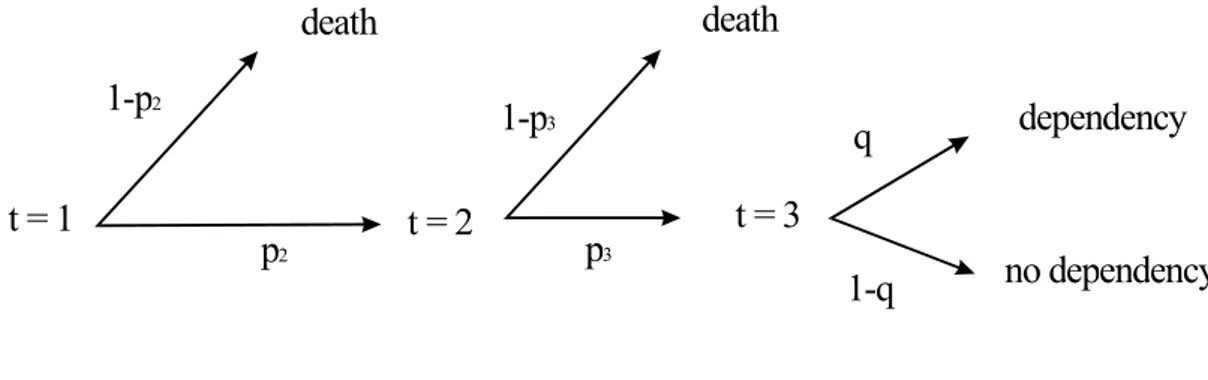
t = 1 death 1-p2 p2 p3 1-p3 t = 2 t = 3 death dependency no dependency q 1-q

Figure 1: The timing.

two periods. Individuals are exposed to two risks: death and long-term care (see figure 1). At t = 1, each agent has a survival probability equal to p2, and a probability to die equal to 1− p2. At the beginning of period 2, each agent survives with a probability equal to p3 till the end of period 2, and the complementary probability to die equal to 1_−p3. If he survives, he may suffer from long-term care with probability equal to q. For the sake of simplicity, we assume that individuals only care for consumption at different periods and in different states of nature, that there is no altruism. Let us denote c1 and c2 consumptions in periods 1 and 2, while consumption in period 3 is indexed on the state of nature : cd

3 and cnd3 (d for dependency and nd for no dependency). Preferences are described through a time-separable expected utility function :

u(c1) + βu(c2) + β2u(c3) (1) where u refers to an instantaneous strictly concave and increasing utility function, and a factor of time preference β - 0 < β < 1. In order to give ex-plicit solutions, we assume a constant elasticity of intertemporal substitution and so :

u(ct) = 1 1_{− σ}(ct)

1−σ ₍₂₎

To deal with risks and to save, individuals trade-off between three finan-cial assets : a riskless asset with return r, annuities, and a long-term care

insurance contract. Annuities perceived in period t are contracts signed in period t_{−1, that provide a gross return ρ if the agent is still alive in period t.} In period 1, individuals perceive an income equal to y1 > 0. They consume c1, and save a2 in annuities. In period 2, they retire and have no exogenous income. They consume c2 and save a3 in annuities. In period 3, they live their last retirement period. They are exposed to the risk of dependency, which incurs a potential extra-consumption (long-term care expenditure).

3

Constraints

We assume a perfect competition insurance market. So, if there is no loading factor, the gross return ρt on annuities thus depends on the riskless interest rate, and the survival probability, and is given by :

ρt= 1 + r

pt

(3) If we assume a loading factor, the return on the annuity market is a more complex function of the interest rate and the survival probability :

t(pt)ρt = 1 + r

where t() is a loading function. When the elasticity of return with respect to survival probability, γ, is held constant, we may assume the following relationship:

ρ_t= (1 + r) p−γt (4)

In period 3 (and only in this period), individuals may suffer from a depen-dency risk which implies more consumption (long-term care expenditures). As shown in figure 1, this risk occurs with probability q and may be covered on a perfect competition insurance market (no loading).

All these assumptions lead to the following budget constraints. In period 1, the representative agent consumes and saves through an annuity contract:

In period 2, if the agent has survived, his budget constraint is similar, his income being now ρ₂a2:

c2+ a3 = ρ2a2 (6)

In the last period, the agent has to determine his desired consumptions in both the dependency state and the nondependency state, and his desired coverage I of the health risk:

cd3+ ηI = ρ3a3+ I− δ (7)

cnd3 + ηI = ρ3a3 (8)

I being the insurance indemnity, and η the unit premium.

Using the completeness property and reasoning backward, we characterize the set of feasible consumptions in each period. From (8) we get:

I = 1

1_{− η}

h

cd₃ + δ_{− ρ3}a3

i

Substituting this result in the second budget constraint of the last period, we get the second period constraint :

cnd3 + η 1_{− η} h cd3+ δ− ρ3a3 i = ρ3a3 or : ηcd₃ + (1_{− η) c}nd₃ = ρ3a3− ηδ (9) This budget constraint can be in turn introduced in the second period budget constraint and so on. After the relevant substitutions, we finally get the intertemporal budget constraint:

c1+ 1 ρ2 c2+ η ρ2ρ3 cd₃ +1− η ρ2ρ3 cnd₃ = y1− η ρ2ρ3 δ

In our framework, the representative agent must choose the assets a2, a3, and I, which enable him to reach his optimal consumption level in each period. Let Ptdenote the survival probability in period t (as of the beginning

of the first period). The optimal consumption levels are solutions of :                                 

maxctu(c1) + βP2u(c2) + qP3β

2_u(cd 3) + (1− q)P3β2u(cnd3 ) subject to : c1+_ρ1 2c2+ η ρ2ρ3c d 3+ρ1−η2ρ3c nd 3 = y1− _ρη 2ρ3δ ct≥ 0, t = 1, 2, 3 The first order conditions are :

                                     βP2 ³_c 1 c2 ´σ = _ρ1 2 β2qP3 µ c1 cd 3 ¶σ = _ρη 2ρ3 β2(1_{− q)P}3 µ c1 cnd 3 ¶σ = _ρ1−η 2ρ3 c1+_ρ1 2c2+ η ρ2ρ3c d 3+ρ1−η2ρ3c nd 3 = y1− _ρη 2ρ3δ (10)

How does the increase in life-expectancy (i.e. the increase in P2 and/or P3) modify the demand for assets a2, a3 and I? What is the impact of dependency risk on these demands? We answer these questions in two steps: first, in a standard framework à la Yaari (that is with no loading and no dependency risk); second, in a framework with dependency risk; and finally, with the introduction of a loading factor.

4

The impact of an increase in life-expectancy

on saving

With no loading and no uncertainty on future consumption, the sequential constraints are :

c2+ a3 = 1 + r p2 a2 (12) c3 = 1 + r p3 a3 (13)

The intertemporal budget constraint is thus : c1+

P2 1 + rc2+

P3

(1 + r)2c3 = y1 (14)

Given the above assumed utility function, the program of the representative

agent is : _                                

maxctu(c1) + βP2u(c2) + P3β

2_u(c 3) subject to : c1+_1+rP2 c2+_(1+r)P3 2c3 = y1 ct≥ 0, t = 1, 2, 3 (15)

At the optimum, we get the following first order conditions:

                     u0_(c 2) = _(1+r)β1 u0(c1) u0_(c 3) = _(1+r)12_β2u0(c1) c1+_1+rP2 c2+ _(1+r)P3 2c3 = y1 (16)

If we assume an isoelastic utility function such as the power function, we

get: _                     c2 = [(1 + r) β] 1 σ _c 1 c3 = [(1 + r) β] 2 σ c 1 c1+_1+rP2 c2+ _(1+r)P3 2c3 = y1 (17)

and : _                                 c1 = 1 1+P2 h (1+r)1σ −1βσ1 i +P3 h (1+r)σ −11 βσ1 i2y1 c2 = [(1+r)β] 1 σ 1+P2 h (1+r)1σ −1βσ1 i +P3 h (1+r)σ −11 βσ1 i2y1 c3 = [(1+r)β] 2 σ 1+P2 h (1+r)1σ −1βσ1 i +P3 h (1+r)σ −11 βσ1 i2y1 (18)

The completeness of markets and the complete diversification of risks imply that consumption levels only depend on the discount factor, the return on the risk-free asset, and the survival probabilities. The higher p2 and p3, the lower the returns on annuities, or equivalently, the higher the cost of consumption in each period. An increase in survival probabilities thus imply a monotonic decrease in the consumption levels.

The consumption functions and the budget constraints give a more de-tailed characterisation of the financial behaviour. With a little algebra, we derive the following demands for assets :

a2 = P2 h (1 + r)σ1−1β 1 σ i + P3 h (1 + r)1σ−1β 1 σ i2 1 + P2 h (1 + r)σ1−1_βσ1 i + P3 h (1 + r)σ1−1_βσ1 i2y1 a3 = 1 + r P2 a2− c2 = (1 + r)µh(1 + r)1σ−1_β1σ i + p3 h (1 + r)σ1−1_βσ1 i2¶ − [(1 + r) β]1σ 1 + P2 h (1 + r)σ1−1_βσ1 i + P3 h (1 + r)σ1−1_βσ1 i2 y1 = (1 + r)p3 h (1 + r)1σ−1β 1 σ i2 1 + P2 h (1 + r)σ1−1_βσ1 i + P3 h (1 + r)σ1−1_βσ1 i2y1

Defining the demands as percentages of income, a2/y1 et a3/y1: a2 y1 = P2 h (1 + r)1σ−1_β 1 σ i + P3 h (1 + r)σ1−1_β 1 σ i2 1 + P2 h (1 + r)1σ−1_βσ1 i + P3 h (1 + r)1σ−1_βσ1 i2

a3 y1 = (1 + r)p3 h (1 + r)σ1−1_β1σ i2 1 + P2 h (1 + r)1σ−1β 1 σ i + P3 h (1 + r)1σ−1β 1 σ i2 We have the following comparative static results :

• An increase in survival probabilities implies an increase in initial accu-mulation a2/y1;

• An increase in the survival probability P2 decreases the third period accumulation a3/y since it reduces the return of the early retirement saving, which in turn reduces further saving;

• An increase in p3 leads to an increase in saving in the first period of retirement, which is fairly intuitive.

We thus obtain the standard results of the literature [4] : since the in-crease in survival probabilities lengthens the agent’s life horizon, it inin-creases the value of saving; the intertemporal smoothing motive induces an increase in the demand for annuities when the agent retires. The theoretical message of our basic framework is in line with the intuition of the standard life-cyle model (which is indeed not surprising since the only risk taken account at that stage in the survival risk). Beyond this period, an increase in the life horizon may have opposite effects on saving: with a given return on the risk-free asset, an increase of the survival probability P2 diminishes the re-turn of annuities, and thus reduces the amount than can be reinvested in the following period ρ2a2.

5

Long-term care and financial behaviour

We now introduce a dependency risk at older age, which take the form of an extra-consumption in period 3 when the risk occurs. Intertemporal smooth-ing is no longer the only motive for savsmooth-ing : long-term care adds a precaution-ary motive in the representative agent’s saving behaviour. Formally, without loading :

ρ₂ = p2

1 + r, ρ3 = p3

the intertemporal budget constraint is: c1+ P2 1 + rc2+ qP3 (1 + r)2c d 3+ (1_{− q)P}3 (1 + r)2 c nd 3 = y1 − qP3 (1 + r)2δ

Since we assume an instantaneous power utility function, the first order con-ditions for an optimal behaviour are :

                                 c2 = [(1 + r) β] 1 σ _c 1 cd 3 = [(1 + r) β] 2 σ _c 1 cnd 3 = [(1 + r) β] 2 σ _c 1 c1 +_1+rP2 c2+_(1+r)qP32cd₃+ (1−q)P 3 (1+r)2 cnd₃ = y1−_(1+r)qP32δ (19)

We find the standard result of the demand for insurance in a perfect com-petition setting: the agent demands full insurance at fair odds. With full insurance, the costs of consumption profiles are held constant :

c3 = cnd3 = c d 3 = [(1 + r) β] 2 σ _c 1

Long-term care has the only impact of reducing the agent’s wealth. Optimal consumption behaviour is given by :

                                 c1 = 1 1+P2 h (1+r)σ −11 βσ1 i +P3 h (1+r)σ −11 βσ1 i2 ³ y1− _(1+r)qP32δ ´ c2 = [(1+r)β] 1 σ 1+P2 h (1+r)σ −11 _βσ1 i +P3 h (1+r)σ −11 _βσ1 i2 ³ y1− _(1+r)qP32δ ´ c3 = [(1+r)β] 2 σ 1+P2 h (1+r)σ −11 βσ1 i +P3 h (1+r)σ −11 βσ1 i2 ³ y1− _(1+r)qP32δ ´ (20)

The dependency risk occurring in period 3 increases accumulation in the first period of the life-cycle :

a2 = y1− c1 = P2 h (1 + r)σ1−1β 1 σ i + P3 [(1+r)β]σ1+qδ y1 (1+r)2 1 + P2 h (1 + r)σ1−1_βσ1 i + P3 h (1 + r)σ1−1_βσ1 i2y1

the higher the survival probability P3 the greater the amount of saving in period 1. The dependency risk also modifies the accumulation pattern in period 2. a3 = 1 + r P2 a2 − c2 = P3 P2(1 + r) h (1 + r)σ1−1_β1σ i2 + (1 + [(1 + r) β]1σ₎ qP3 (1+r)2 δ y1 1 + P2 h (1 + r)σ1−1_β 1 σ i + P3 h (1 + r)σ1−1_β 1 σ i2 y1 With a low probability of being dependent, the demand for annuities incre-sases with the survival probability in period 3 other things being equal.

The impact of the survival probabilities P2 and P3, along with the depen-dency probability q, on the demand for annuities more difficult to forecast, since these probabilities are basically determined by the same variable (the health state of the population). An improvement of agent’s health has thus two opposite effects on probabilities: it reduces the dependency probability (q) but increases life horizon (increasing P2 and P3).2 We have theoretically shown that an improvement of “life perspectives” has the two saving motives playing in an opposite way, the intertemporal smoothing motive reducing accumulation, while the precautionary pushes it up.

6

Robustness

What is the effect of a loading factor in the pricing of annuities? We show that introducing an implicit loading factor does not qualitatively modify our previous results. The loading assumption is introduced through a constant elasticity of returns vis-à-vis the survival probabilities :

ρ_t = (1 + r)p−γt

2_{This is an empirical observation: the increase in life-expectancy seems to be positively}

The preceding optimal conditions are modified as follows: c1 = y1− _ρη 2ρ3δ 1 + ρ 1 σ−1 2 (βP2) 1 σ ₊ η ρ₂ρ₃ ³_ρ 2ρ3β2qP3 η ´1 σ +_ρ1−η 2ρ3 ³_ρ 2ρ3β2(1−q)P3 1−η ´1 σ If we denote : g(Pt) = (Pt) 1+γ(σ−1) σ then : c1 = y1− q(1 + r)2P3−γδ 1 + g(P2) h (1 + r)1−σβi 1 σ + g(P3) h (1 + r)1−σβi 2 σ As : _         ((1 + r)β)σ1 _P 1−γ σ 2 c1 = c2 ((1 + r)β)σ2 _P 1−γ σ 3 c1 = c3 (21) we obtain : c2 = (1 + r)P₂−γg(P2) h (1 + r)1−σβi 1 σ 1 + g(P2) h (1 + r)1−σβi 1 σ + g(P3) h (1 + r)1−σβi 2 σ ³ y1− q(1 + r)−2P3γδ ´ c3 = (1 + r)2_P−γ 3 g(P3) h (1 + r)1−σβi 2 σ 1 + g(P2) h (1 + r)1−σβi 1 σ + g(P3) h (1 + r)1−σβi 2 σ ³ y1− q(1 + r)−2P3γδ ´

We test the robustness of our previous conclusions on comparative statics. Assume a coefficient of relative risk aversion above 1, then the g function is strictly increasing. g0(Pt) = 1 + γ(σ_{− 1)} σ (Pt) (γ−1)(σ−1) σ _{> 0 if σ > 1}

With no dependency risk, an increase in survival probabilities (P2 and P3) leads to a higher saving rate, other things being equal. Moreover, if we assume and γ > 1, the g function is strictly convex. We then get the same conclusions as Levhari and Mirman (1977) [3] : if the (P0

t) probability distribution is second-order dominated by (Pt) :

t X i=1 Pi > t X i=1 Pi0

Figure 2: Impact of the dependency probability (p3)on the first period saving rate (a2/y1)- with q = 0, 0.1, 0.2, 0.5.

then a2/y1 will be higher under (Pt). The saving behaviour in period 2 has the same property than in the perfect competition case, since :

a3 y1 = (1 + r)P −γ 2 g(P3) h (1 + r)1−σβi 2 σ 1 + g(P2) h (1 + r)1−σβi 1 σ + g(P3) h (1 + r)1−σβi 2 σ

The demand for annuities in period 2 decreases with P2, and increases with P3.

If the dependency risk were taken into account, we would reach the same conclusions as before: the saving behaviour would be determined by the precautionary motive along with the intertemporal smoothing motive. This can be illustrated by numerical simulations, with

p2 = 0.8, q = 0.1, r = 5%, β = 0.8, σ = 5, γ = 1.2, δ y1

= 0.5

These simulations (figures 2, 3, 4, 5) show that the saving behaviour in each period is hardly modified when the dependency risk is introduced.

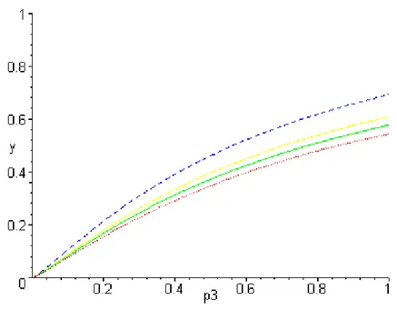
Figure 3: Impact of the dependency probability (p3) on the second period saving rate (a3/y1)- with q = 0, 0.1, 0.2, 0.5.

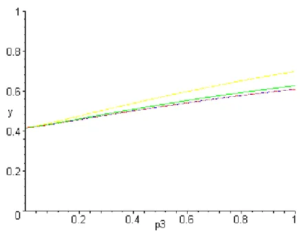
Figure 4: Impact of the dependency probability (p3)on the first period saving rate (a2/y1)- with δ/y1 = 0, 0.5, 1

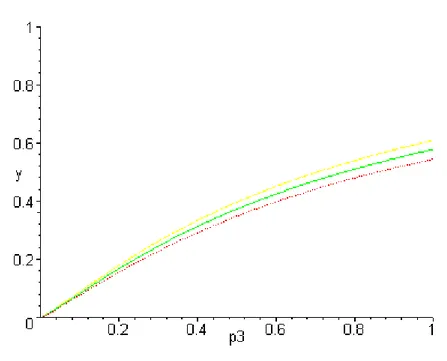
Figure 5: Impact of the dependency probability (p3) on the second period saving rate (a3/y1)- with δ/y1 = 0, 0.5, 1

7

Conclusion

On a theoretical ground, there are several arguments in favour of an in-crease of retirement saving at old ages. Contrary to the standard life-cycle model, individual ageing does not necessarily imply dissaving or a reduc-tion of financial risk taking. We have shown in this paper that an increase in life-expectancy may increase saving at older ages, when individuals have two saving motives, that is intertemporal smoothing and precautionary mo-tives. We have computed simulations with plausible parameters related to risk-aversion, time preference and returns, and we have shown that the in-tertemporal smoothing motive is dominating.

These theoretical results are in line with empirical findings in the French case. Indeed, in a previous paper, we showed that French households still continue to save when they retire (Bernard et al. (2002) [2]) . Using a probit estimation on the demand for endowment insurance and retirement saving, we found that individuals belonging to the 60-74 age group have a

signifi-cantly higher proportion of their financial wealth in endowment insurance, annuities and voluntary retirement saving than people under 60. Using an OLS regression, we also found that the proportion of endowment insurance, annuities and voluntary retirement saving in financial wealth is higher for older individuals, other thing being equal. These empirical findings give some support to our theoretical framework.

References

[1] P. Artus, (2002). Profil de l’épargne pendant la retraite et équilibre financier. working paper, Caisse des Dépôts et Consignations, Paris, Mai 2002.

[2] Ph. Bernard, N. Mekkaoui de Freitas, A. Lavigne, and R. Mahieu, (2002). Ageing and the demand for life insurance : an empirical investigation using french panel data. working paper, Université Paris Dauphine and Université d’Orléans, December 2002.

[3] D. Levhari and L.J. Mirman, (1977). Consumption and saving with an uncertain horizon. Journal of Political Economy, 85:265—81, 1977. [4] M. Yaari, (1965). Uncertain lifetime, life insurance, and the theory of the