Laboratoire d’Economie de Dauphine
WP n°7/
2014
Mathilde Godard
(CREST and Université Paris Dauphine)
08
Autom
ne
Document de travail
Gaining weight through retirement?
Gaining weight through retirement? Results from
the SHARE survey
∗Mathilde Godard†
CREST and University Paris-Dauphine, LEDa-LEGOS
March 2014
Abstract
This paper estimates the causal impact of retirement among the 50-69 year-old on Body Mass In-dex (BMI), the probability of being either overweight or obese and the probability of being obese. Based on the 2004, 2006 and 2010-11 waves of the Survey of Health, Ageing and Retirement in Eu-rope (SHARE), our identification strategy exploits the EuEu-ropean variation in Early Retirement Ages (ERAs) and the stepwise increase in ERAs in Austria and Italy between 2004 and 2011 to produce an exogeneous shock in retirement behaviour. Our results show that retirement induced by discontinuous incentives in early retirement schemes causes a 13 percentage point increase in the probability of being obese among men within a two to four-year period. Additional results show that this effect is driven by men having retired from strenuous jobs and who were already at risk of obesity. No effects are found among women.
Keywords : Body Mass Index; Obesity; Retirement; Instrumental Variables
JEL code : I10, J26, C26
∗
I wish to thank Andrea Bassanini, Luc Behagel, Eve Caroli, Cl´ementine Garrouste, Cl´ement de Chaise-martin, Brigitte Dormont, Peter Eibich, Fabrice Etil´e, Florence Jusot, Anne Laferr`ere, Pascale Lengagne, Maarten Lindeboom, Claudio Lucifora, Mathilde Peron, Roland Rathelot, and seminar participants at the University Paris-Dauphine, CREST LMi-LabEval and Leeds Academic Unit of Health Economics seminars as well as to the TEPP Public Policy Evaluation Winter School in Aussois, the JMA conference in Nice, the 4th SHARE User Conference and the IZA workshop on labor markets and labor markets policies for older workers in Bonn for useful comments and suggestions. I am grateful to Nicolas Sirven and Nicolas Briant for sharing with me their thorough knowlegde of the SHARE survey. This paper uses data from SHARE wave 4 release 1.1.1, as of March 28th 2013 and SHARE waves 1 and 2 release 2.5.0, as of May 24th 2011. The SHARE data collection has been primarily funded by the European Commission through the 5th, the 6th and the 7thFramework Programme. Additional funding from the U.S. National Institute on Ageing and the German Ministry of Education and Research as well as from various national sources is gratefully acknowledged (see www.share-project.org for a full list of funding institutions).
†CREST, 15 Boulevard Gabriel P´eri, 92245 MALAKOFF Cedex. Phone : +0033(0)141175902. E-mail :
1
Introduction
In its 1998 report, the World Health Organization (WHO) ranked the obesity epidemic among the leading ten global public health issues. Obesity rates in the world have more than doubled over the last 30 years (WHO (2012)). In the 27 European Union member states, approx-imately 60% of the adult population – 260 millions of adults – is either overweight (Body Mass Index (BMI) from 25 to 29.9 kg/m2) or obese (BMI 30 kg/m2 and above) (International Obesity Task Force (IASO/IOTF (2010)). Obesity has become a pan-European epidemic (IASO/IOTF (2002)) and prevalence rates in the EU-27 range from 7.9% in Romania to 24.5% in the United-Kingdom (OECD (2010)).
Obesity is a risk factor for numerous highly-prevalent and costly chronic diseases (car-diovascular diseases, type-2 diabetes, hypertension and certain types of cancer) and for dis-ability. It reduces the quality of life, shortens life expectancy and lowers the levels of labour productivity (Must et al. (1999); Rosin (2008)). Moreover, it places a heavy financial burden on the individual and on society – particularly on public transfer programmes and private health plans (Finkelstein et al. (2003)). At the individual level, Emery et al. (2007) find that healthcare costs for French obese individuals are on average twice the costs for normal-weight individuals. At the aggregate level, obesity-related healthcare expenditures account for 1.5 to 4.6% of total health expenditures in some European countries (see Schmid et al. (2005) and Emery et al. (2007) for evidence on France and Switzerland respectively).
In most European countries, obesity rates reach their peak around age 60.51 (Sanz-de Galdeano (2005)). Recent studies have highlighted the particularly strong impact of over-weight, obesity and increased BMI on morbidity and disability among adults aged 50 and older (Andreyeva et al. (2007); Peytremann-Bridevaux and Santos-Eggimann (2008)), thereby attracting policymakers’ attention to the substantial burden that obesity places on the gen-eral health and autonomy of adults aged over 50.
Understanding the causes of obesity among the elderly is therefore a key issue. Unlike other age groups – such as children or adolescents – it hasn’t received much attention yet. As the elderly are characterised by low labour participation and high job-exit rates, one might wonder whether transitions out of employment have an impact on the weight trajectories of individuals aged 50 years and older. In this paper, we focus on the most common transition out of employment, i.e, retirement.
There are some reasons to believe that retirement might trigger weight changes. The Grossman model of the demand for health (Grossman (1972)) is consistent with the inter-pretation that individuals are likely to adopt health-producing activities – such as physical
1
This figure does not allow us to disentangle age and cohort effects. Using the 2004, 2006 and 2010 waves of the Survey of Health, Ageing and Retirement in Europe (SHARE), we find that obesity rates among the 50-70-year-old reach their peak between age 55 and 65 for all cohorts born between 1940 and 1954.
exercise or healthier diets – after retirement : although retirees have a tighter budget con-straint, they have more time to allocate to leisure. Empirical findings seem to corroborate this view. In a three-year follow-up of French middle-aged adults, Touvier et al. (2010) find that retirement is associated with an increase in leisure-time physical activities of moderate intensity, such as walking. As for food intake, finding are more mixed. On US longitudinal data, Chung et al. (2007) find that households spend less on eating out ($10 per month on average) following retirement, while their monthly spending on food at home does not change. In a recent review of the literature, however, Hurst (2008) argues that due to an increase in food home production, the overall food intake does not decline following retirement. Over-all, these results suggest that retirement would rather operate on weight through changes in physical activity than via food consumption.
At the same time, new retirees may lose some incentive to invest in health as their income is no longer dependent on health : once retired, their pension benefits do not depend on health. This could lead to lower health investments, and to a lower health stock in the long-run. Besides, retirement might also increase the risk of social isolation and depression (Friedmann and Havighurst (1954); Bradford (1979)), leading individuals to potentially re-duce their efforts in health-producing activities and develop addictive behaviours (alcohol or tobacco consumption). Finally, the loss of a structured use of time may also encourage snacking in-between meal times and sedentary habits (television watching). In the study mentioned before, Touvier et al. (2010) find that retirement is also associated with an in-crease in time spent watching TV.
Overall, the direction of the effect is not clear. More specifically, it is likely to be highly heterogeneous, in particular across job types. As retirement induces a direct reduction in job-related exercise, individuals having retired from strenuous jobs are at a higher risk to gain weight if they do not compensate by increasing their leisure-time physical activity or by decreasing their food intake. Conversely, retirees from sedentary jobs may lose weight if their leisure-time activities after retirement are more physically demanding than time at work.
The purpose of the present paper is to estimate the causal impact of retirement on BMI, the probability of being either overweight or obese and the probability of being obese. Iden-tifying such a causal impact is problematic in the presence of confounding factors and reverse causality. Retirement is indeed often a choice, and often based on unobservable characteris-tics which may be correlated with weight (time preference2, health or psychological deterio-rations). Reverse causality may also be a concern. As overweight and obese individuals are on average paid less, less promoted (Cawley (2004); Morris (2006); Brunello and d’Hombres (2007); Schulte et al. (2007)) and in worse health, their incentives to retire might be higher than normal-weight individuals. Burkhauser and Cawley (2006) show that fatness and obe-sity are indeed strong predictors of early receipt of old-age benefits in the USA.
To tackle this endogeneity issue, we use an instrumental variable approach. Our
iden-2
See Smith et al. (2005), Anderson and Mellor (2008) and Ikeda et al. (2010) for empirical evidence of the positive relationship between time preference and BMI.
tification strategy exploits the fact that as individuals reach the Earliest Retirement Age (ERA) at which they are entitled to either reduced pensions or full pensions – conditional on a sufficient number of years of social security contributions – the probability that they retire strongly increases. Said differently, this discontinuous incentive in the social security system provides a strong exogeneous shock on retirement behaviour. We exploit the variation in ERAs across European countries as well as its variation over time (in countries that imple-mented a stepwise increase in the ERA during the period under study) to solve the major identification problems related to confounding factors and reverse causality. We implement a fixed-effect instrumental variable model in order to control for both time-invariant factors (such as genetics) and time-varying ommited variables and/or reverse causality. We finally estimate the short-term causal effect of a transition to retirement on weight. We use the 2004, 2006 and 2010 waves of the Survey of Health, Ageing and Retirement in Europe (SHARE). Our results show that retirement causes a 13 percentage point increase in the probability of being obese within a two to four-year period3 among men. Additional results show that this effect is driven by men having retired from strenuous jobs and who were already at risk of obesity. No effects are found among women.
This paper relates to several strands of literature. First and foremost, it contributes to the literature on the effects of retirement on weight. Most papers in the literature on this topic estimate mere correlations, disregarding the possibility that retirement be endogenous. Re-sults have been quite consistent so far. Nooyens et al. (2005) find that the effect of retirement on changes in weight and waist circumference depends on one’s former occupation : weight gain is higher among men who retired from an active job. Forman-Hoffman et al. (2008) find no significant relation for men, but a weight gain for women retiring from blue-collar jobs. Gueorguieva et al. (2010) find a significant increase in the slopes of BMI trajectories only for individuals retiring from blue-collar occupations. To the best of our knowledge, Chung et al. (2009) and Goldman et al. (2008) are the only studies tackling the endogeneity issue. Both use longitudinal data from the Health and Retirement Study – the US equivalent of the European SHARE survey – and estimate fixed-effect models. They use social security and Medicare eligibility (ages 62 and 65 respectively) as instruments for retirement.4 Chung et al. (2009) conclude that people already overweight and people with lower wealth retiring from physically-demanding occupations suffer from a modest weight gain. Goldman et al. (2008) find that males retiring from strenuous jobs gain weight (by 0.5 units of BMI) during the first six years of retirement, while those retiring from sedentary jobs lose some. We improve with respect to this literature in three respects : first, we identify a causal effect of retire-ment on weight, while most papers docuretire-ment a mere correlation. Second, the variation in ERAs across Europe and over time allows us to explore the effect of retirement on weight at
3There is a two-year period between the 2004 and 2006 waves of SHARE and a four-year period between waves 2006 and 2010.
4
Chung et al. (2009) also use spouse pension eligibility as an additional instrument. However, recent work highlights asymmetries in spouses retirement strategies (Gustman and Steinmeier (2009); Stancanelli (2012)). Using spouse pension eligibility as an additional instrument might thus be a questionable strategy.
different ages, not just ages 62 and 65, as in Chung et al. (2009) and Goldman et al. (2008). Moreover, weaker assumptions in terms of weight trajectories by cohort and age are needed in our empirical setup. Finally, our paper is the first one to exploit European data. Most of the above-mentioned studies – except Nooyens et al. (2005) – use US data from the Health and Retirement Survey (HRS). Given the differences in terms of labour markets, social security schemes and social policies, it is not clear whether the results obtained for the USA should hold for Europe.
This paper also relates to a substential recent literature that explores the effects of retirement on health and related outcomes – mental health, cognitive functioning and well-being. This literature indulges its best to take into account the endogeneous nature of retirement. Recent papers have exploited discontinuous incentives in social security systems as exogeneous shocks in retirement decisions (Charles (2004); Neuman (2008); Coe and Lindeboom (2008); Coe and Zamarro (2011)5; Rohwedder et al. (2010); Behncke (2011); Bonsang et al. (2012); Blake
and Garrouste (2012); Eibich (2014)) as we do. However, the results in this literature are still ambiguous, and whether or not retirement has a detrimental effect on health is still an open debate. As weight change is likely to be an important mechanism by which retirement affects health, this paper contributes to this recent and growing literature by exploring one of the potential mediating channels between retirement and health.
Finally, this paper contributes to a growing body of literature that investigates the impact of various dimensions of professional activity on body weight and obesity, such as papers focusing on unemployment (Marcus (2012)), working conditions (Lallukka et al. (2008b)), occupational mobility (Ribet et al. (2003)), job insecurity (Muenster et al. (2011)), physical strenuousness at work (B¨ockerman et al. (2008)), working overtime (Lallukka et al. (2008a)), and income (Cawley et al. (2010), Schmeiser (2009), Colchero et al. (2008)).
The paper develops as follows. Section 2 presents our empirical approach and Section 3 describes the data (the 2004, 2006 and 2010 waves of SHARE). Section 4 presents the results and Section 5 provides some conclusions.
2
Empirical approach
We investigate the impact of retirement on BMI, the probability of being either overweight or obese and the probability of being obese. As a first step, we pool the observations from the 2004, 2006 and 2010 waves of the SHARE survey and estimate the following equation by
5Our identification strategy is similar in spirit to Coe and Zamarro (2011), who use the 2004 wave of SHARE and use country-specific early and full retirement ages as instruments for retirement behaviour. However, we improve with respect to this paper in two respects. First, we take advantage of the panel structure of the SHARE data, which allows us to control for individual time-invariant unobservable characteristics. Then, we exploit the European variation in early retirement schemes as well as reforms in early retirement ages in Austria and Italy over the 2004-2011 period to produce an exogeneous shock in retirement. Finally, rather than investigating the effect of retirement on health, we investigate the effect of retirement on an under-investigated dimension of health and a major risk factor for numerous diseases among the elderly, i.e, weight change and obesity.
a standard Pooled Ordinary Least Squares (POLS) model :
Yit= α + γRit+ Xitβ + Di+ Dt+ uit (1)
where Yit denotes the weight outcome of individual i at time t.6 Rit is a binary variable
indicating whether individual i is retired at time t, Xit a vector of individual characteristics
either time-varying or time-invariant, Di a country dummy, Dt a time dummy and uit the
error term.
However, the retirement status Rit can potentially be correlated with the error term uit,
in which case the POLS estimate of γ is inconsistent. Endogeneity may arise from several sources. Omitted variables, such as unobservable time preference or health deteriorations may have an impact both on the probability of retiring and on weight changes. Similarly, reverse causality may also be a concern : obese individuals are more likely to seek early retirement benefits (Burkhauser and Cawley (2006)).
Faced with these endogoneity problems, we consider a Fixed-Effects (FE) model such as :
Yit= α + γRit+ Kitβ + Dt+ αi+ vit (2)
where Yitstill denotes the weight outcome, Rit the individual retirement status, Kita vector
of time-varying individual characteristics, Dt a time dummy, αi an individual fixed-effect –
including the country fixed-effect – and vit the error term.
The FE model allows regressors to be endogeneous, provided that they are correlated only with αi, the time-invariant component of the error, but not with the idiosyncratic error vit. If
some unobservable time-varying characteristics are correlated with Rit, however, ˆγ continues
to be biased. Moreover, reverse causality is still a concern.
In order to tackle the endogeneity problem, we estimate a Fixed-Effect Instrumental Vari-able (FEIV) model. This model allows us to control for both time-invariant factors (such as genetics, food preferences over the life-course or time preference) and time-varying ommited variables as well as reverse causality. Our identification strategy exploits the fact that as individuals reach the Earliest Retirement Age (ERA) in their countries, the probability that they retire strongly increases. This exogeneous shock in retirement behaviour allows us to estimate the causal impact of a transition to retirement on weight in the short-run – within a two to four-year period.
Retirement decisions in industrialised countries depend on a number of institutional fea-tures. In particular, the earliest age at which individuals are entitled to pension benefits has been shown to exert a powerful influence on their retirement behaviours (Gruber and Wise (1999)). This ERA is defined as the earliest age at which individuals are entitled to
6
Yitcan be either continuous (the BMI) or binary (being either overweight or obese/being neither overweight nor obese; being obese/not being obese). POLS (presented) and pooled probit models yield very similar results when the dependent variable is binary.
either reduced pensions or full pensions – conditional on a sufficient number of years of so-cial security contributions. The Offiso-cial Retirement Age (ORA) is the age at which workers are entitled to either minimum-guaranteed pensions or full old-age pensions irrespective of their contributions or work histories. It appears to be typically less important in predicting retirement behaviour than the ERA (Gruber and Wise (1999)). Few individuals actually work until the official retirement age. As a consequence, there is a gap between the official retirement age and the average effective age at which older workers withdraw from the labour force in almost all industrialised countries.
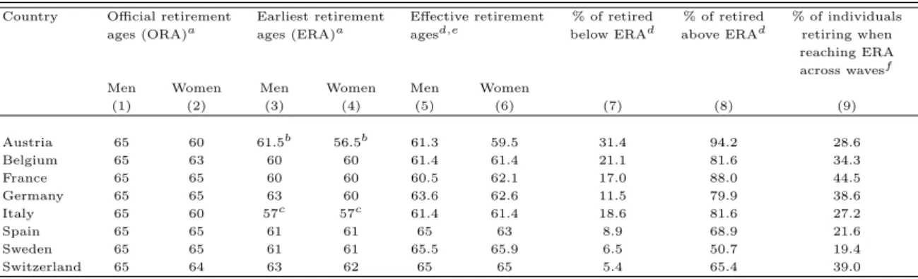
Earliest, official and effective retirement ages in Europe are presented in Table 1. As evidenced in columns 1 and 2, the official retirement age varies very little across countries and genders. In contrast, the ERA varies quite a lot across countries and genders (columns 3 and 4). Effective retirement ages are lower than official retirement ages in almost every country (see columns 5 and 6 for men and women respectively). A number of countries in our sample implemented substantial reforms in ERAs over the period under study. In Austria for instance, the 2004 pension reform introduced a gradual increase in the ERAs for men and women. Immediatly before the reform, workers in Austria could still retire at ages 61.5 (men) and 56.5 (women). After the reform, the ERAs were increased by two months for each quarter of birth for men born in the first two quarters of 1943 and women born in the first two quarters of 1948. Following these increases, the ERAs were increased by one month for each quarter of birth for men born in the third quarter of 1943 and later and for women born in the third quarter of 1948 and later. Furthermore, the 2004 pension reform also created special corridor pensions for men born in the last quarter of 1943 and later, thereby making the ERA beyond age 62 non-binding in many cases (Manoli and Weber (2012)). Italy also introduced a stepwise increase in the minimum age to request early retirement, from age 57 in 2004 to age 60 in 2011. More information about the Austrian and Italian reforms are available in Table 1.
We take advantage of the ERA variation across countries and over time to explore the causal effect of retirement on weight. We instrument the retirement status Rit by a dummy
variable indicating whether individual i ’s age at time t is above or below the ERA in force at time t in his country c. Let ageit be individual i ’s age at time t and ERAct the ERA in
i ’s country c at time t. Our instrument is defined as :
Zict= 1{ageit>ERAct} (3)
A good instrument should be strongly correlated with actual retirement behaviour but should not directly affect weight outcomes.
As shown in Table 1, Z appears to be well correlated with retirement status. Suggestive evi-dence is provided by columns (7) and (8) : in each country, there is a large gap in the fraction of individuals retired before and after the ERA cutoff. For example, only 17% of individuals in the pooled sample in France are retired before age 60 – when they are first entitled to social security benefits – but this proportion increases to 88% after age 60. Taking advantage of the
panel structure of our data, we then compute for each country the proportion of individuals retiring when reaching their country’s ERA between two subsequent waves of the survey (see column (9)). This proportion is high in most countries. For instance in Belgium, 34.3% of the individuals reaching age 60 between two waves of the survey actually retire between these two waves.
At the same time, once controlling for age, reaching the ERA cutoff is highly unlikely to be correlated with weight outcomes except through the increased probability of retiring. This exclusion restriction holds if we assume there is no discontinuity in the weight trajectories of cohorts at ERAs except for the effect of retirement at these given ages. As we consider different cohorts and since the ERA is both country and time-varying, this assumption is likely to hold in our data. We show in the robustness section that it is the case.
Equation (2) is then estimated by fixed-effect two-stage least squares. In the first stage, the retirement status Rit is regressed on Zit and other covariates. In the second stage,
equa-tion (2) is estimated by a FE regression/FE linear probability model where Rit is replaced
with its predicted value from the first stage. The covariance matrix of ˆγ is corrected accord-ingly.
Our FEIV estimate ˆγ can be given a causal interpretation as a Local Average Treatment Ef-fet (LATE) without requiring constant treatment assumption. In our case, the “treatment” is defined as retiring between two subsequent waves of the survey. More specifically, ˆγ is identified on the subset of individuals whose behaviour is shifted by our instrument, i.e, the compliers. In this setup, compliers are individuals who either became eligible to early retire-ment schemes between two subsequent waves of the survey and did retire then; or individuals whose eligibility to early retirement schemes did not change between two subsequent waves of the survey and who did not retire then. As the ERA is probably more binding for individuals with long careers, we expect compliers to be less educated people.
Overall, our estimation stratgy allows to us to measure the causal effect of a transition to retirement on weight within a two to four-year period among this subpopulation of compliers.
Our empirical setup can be viewed as a fuzzy regression design with multiple discontinu-ities (both country and time-varying). It allows us to explore the effect of retirement on a wide range of ages, not just ages 62 and 65 as in the US studies. Moreover, weaker assump-tions in terms of weight trajectories by cohort and age are needed in this setup.
Finally, as Coe and Zamarro (2011) underline, there do exist other ways to exit the labour force, e.g, through unemployment or disability programmes. However, to the extent that these patterns are stable within countries over the period under study, the individual fixed-effect will pick up this variation and it will not bias our results.
3
Data
3.1 Presentation of the sample
We use data from the Survey of Health, Ageing and Retirement in Europe (SHARE). SHARE is a multidisciplinary and cross-national panel database containing individual information on health, socio-economic status and social and family networks. Approximately 85,000 in-dividuals over 50 years old and their spouses/partners (independent of their age) from 19 European countries (including Israel) have been interviewed so far. By now, four waves have been conducted and further waves are being planned to take place on a biennial basis. We use the 2004, 2006 and 2010 waves of SHARE.7 In order to have a balanced panel, our sample includes the ten European countries that took part in the 2004 SHARE baseline survey and further participated in waves 2006 and 2010, i.e, Austria, Germany, Sweden, The Nether-lands, Spain, Italy, France, Denmark, Switzerland and Belgium.
Our sample contains all individuals interviewed in waves 2004, 2006 and 20108, aged 50 to 69 years old9, who declared in each wave being either employed or retired. In other words, we only consider the traditional and most frequent pattern of retirement, where individuals transit directly from work to retirement. Transitions from employment to unemployment, invalidity or inactivity are thus excluded. We also exclude transitions from retirement to em-ployment, unemem-ployment, invalidity or inactivity. In the empirical analysis we thus compare individuals whose job status remains stable across waves (either retired or employed) and individuals who retire across waves. As there is no early retirement option in Denmark and since early retirement was abolished in 2005 in the Netherlands, both countries are excluded from the analysis. Finally, we exclude individuals reporting a height below 1.20 meters as well as individuals reporting a weight either below 30 kilograms or above 200 kilograms. Over-all, our dataset contains 2703 individuals10 from eight countries (Austria, Germany, Sweden, Spain, Italy, France, Switzerland and Belgium) across the three waves.
3.2 Variables
We use a question on self-declared current job situation to determine whether an individual is retired or not. According to this definition, anyone who declares herself as retired, whether
7
The 2008-2009 wave of SHARE, SHARELIFE, is a retrospective survey that focuses on people’s life histories. Although it can be linked to the existing data of SHARE, it is not of direct use here and we do not use it.
8
We thus consider a balanced panel. Attrition rates are rather high in SHARE. However, high attrition rates are a concern if non response is systematically related to health. De Luca (2009) shows that differential attrition due to health in SHARE is not clear-cut and we conclude that our results are not likely to be systematically biased by differential attrition due to health.
9The 50-69 age window broadly corresponds to the ages at which individuals reach the ERA in their country and become entitled to pension benefits.
10
Once conditioning on having no missing value on weight, height and any covariate included in the model, our sample goes down to 2493 individuals across the three waves (1353 men and 1140 women), i.e, 7479 observations in the pooled sample (4059 men and 3420 women).
she has been or not in a paid job during the month preceding the interview – even for a few hours – is considered as retired. Conversely, anyone who declares herself to be employed or self-employed is considered as currently working. The self-declared retirement status seems to be a reliable information in SHARE : it is strongly associated with the eligibility for either public or private pensions in the dataset.11 We also use an alternative and more restrictive definition of retirement as a robustness check. According to this definition, an individual is considered as retired if (i) his self-declared job situation is “retired” and (ii) he did not do any paid work during the preceding month. Conversely, an individual is considered as employed if his self-declared job situation is “employed or self employed”.12
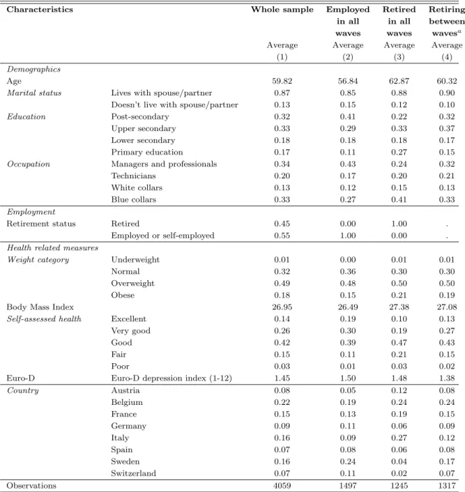
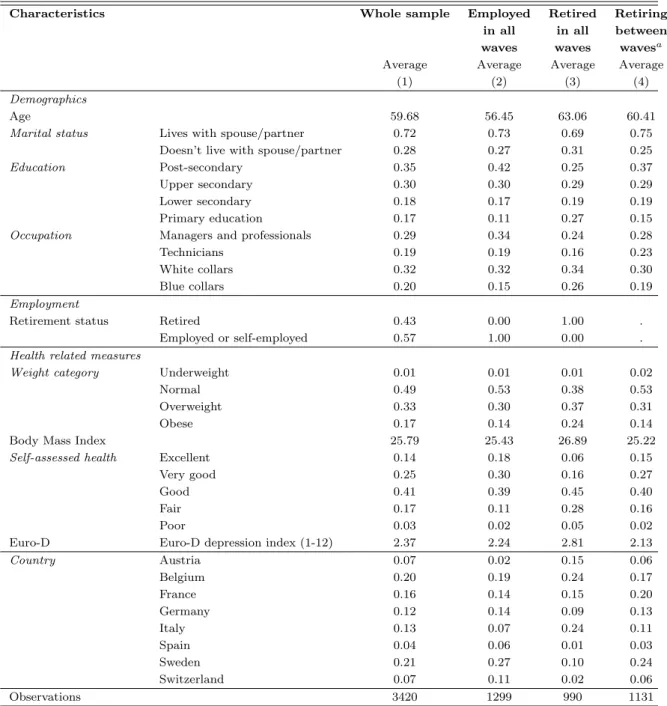
Tables 2 and 3 provide summary statistics for the full sample – pooled over 2004-2010 – for men and women respectively. Each table also presents characteristics for the individu-als either continuously employed across waves (column 2), continuously retired across waves (column 3), or having retired across waves (column 4). According to Tables 2 and 3, 45% of men and 43% of women in the full sample were employed or self-employed, the rest being retired. Eight hundred and sixteen individuals (23% of the individuals working in 2004) re-tired between 2004 and 2010. According to our alternative definition of retirement, only 395 individuals (13% of the individuals working in 2004) retired between 2004 and 2010.
The BMI is calculated in each wave as the self-declared weight in kilograms divided by the square of the self-declared height in meters (kg/m2). We derive clinical weight cate-gories from the BMI : underweight (BMI under 18.5 kg/m2), normal (BMI from 18.5 to 24.9 kg/m2), overweight (BMI from 25 to 29.9 kg/m2) and obese (BMI 30 kg/m2and above). We also compute individual weight change (in kg) as well as a dummy variable indicating if the individual experienced a weight change of at least 10% between two subsequent waves of the survey. The BMI is a rather crude measure of body composition, as it does not distinguish fat from lean mass (Prentice and Jebb (2001); Burkhauser and Cawley (2008)). However, it has been shown to be highly correlated with more precise measures of adiposity. When reported – as it is the case here –, the BMI may additionally suffer from measurement error (Niedhammer et al. (2000); Burkhauser and Cawley (2008)). Following Brunello et al. (2013), we note that the rank correlation between country level self-reported and objective measures of weight is however very high in Europe (Sanz de Galdeano (2007)).
The average BMI of the full sample was 26.95 kg/m2 for men and 25.79 kg/m2 for women, slightly above the overweight threshold in both cases. Eighteen percent of men in the full sample were obese, 49% overweight, 32% normal and less than 1% underweight. As for women, 17% were obese, but less than 33% were overweight and 49% had a normal weight. Interestingly, while only 15% of men employed in all waves were obese, 21% of men retired in all waves were obese. The same pattern was found for women (the corresponding figures
11Among the 3281 individuals retired in the pooled sample, 84% declared that they had received an income from either a public or occupational old age pension during the year preceding the interview.
12SHARE also includes information about the year and the month of retirement. However, this measure is not reliable in our data and we do not use it. Hence, we know if a given individual retires between two waves of the survey, but we do not have any information on the exact month and year of retirement.
are 14% and 24%). This large gap is probably best explained by the fact that individuals employed in all waves are on average younger than individuals retired in all waves. However, it suggests that the 50-69-year-old undergo serious weight change around retirement age. Additional descriptive statistics seem to corroborate this view : in the pooled sample – irre-spective of retirement status –, 11% of individuals experienced a weight change (either gain or loss) of at least 10% between two subsequent waves of the survey. Seventeen percent became either overweight or obese across two subsequent waves of the survey, while 8% either over-weight or obese switched back to a normal over-weight category. More specifically, Figures 1 and 2 suggest that weight change is more important among individuals having retired between waves. Figure 1 plots the distribution of weight change for individuals having retired across waves as well as the distribution of weight change for individuals continuously employed or retired in all waves, for men and women respectively. A simple look at each graph suggests that the distribution is flatter for individuals having retired across waves : the peak around zero – meaning no weight change – is indeed less clear-cut in both graphs. Although the distributions are not significantly different – neither for men nor for women –, it suggests that individuals who retire experience weight change to a higher extent than individuals con-tinuously employed or retired. Similarly, the proportion of individuals experiencing a weight change of at least 10% between two subsequent waves of the survey (see Figure 2) is higher among men and women having retired (11% and 14% respectively) than among men and women continuously employed or retired (9% and 12% respectively).13
Different sets of covariates are used, depending on the specification used (POLS, FE or FEIV models). We introduce age and age squared in all specifications to control properly for the age trend and to account for a potential non-linear effect of age on weight. Each specification also includes marital status (lives with a spouse-partner/does not live with a spouse-partner) and time dummies for 2006 and 2010. The average age of men and women in the pooled sample was 59.8 and 59.7 years old respectively. On average, men and women having retired between 2004 and 2010 were aged 60.3 and 60.4 years old respectively. Eighty-seven percent of men in the full sample lived with a spouse or partner, while only 72% of women did so. Gender, educational level14 (primary education/lower secondary/upper sec-ondary/postsecondary), occupation15 (blue collars/white collars/technicians/managers and
professionals) and country dummies are only included in the POLS specification, as FE and FEIV models do not permit to identify the effects of time-invariant variables. Summary statistics for gender, educational level, occupation and country can be found in Tables 2 and 3 for men and women respectively. Seventeen percent of men in the full sample had achieved primary education, 18% lower secondary education, 33% upper secondary education and 32% post secondary education. The corresponding figures for women are 17%, 18%, 30% and 35%.
13This is only suggestive evidence, given that the two proportions are not statistically different according to the khi-square test (neither for men, nor for women).
14
Based on the 1997 International Standard Classification of Education (ISCED 97) 15
Based on the 1988 International Standard Classification of Occupations (ISCO 88). Occupation is not time-varying in our data. Given that we focus on elderly workers, it seems to be a plausible assumption.
Thirty-three percent of males in the pooled sample were in blue-collar occupations, 13% in white-collar occupations, 20% were technicians and 34% managers or professionals. Simi-larly, 20% of women in the full sample were in blue-collar occupations, 32% in white-collar occupations, 19% were technicians and 29% managers or professionals. Men and women having retired across waves exhibited the same patterns of education and occupation than individuals in the full sample. Belgium, Sweden, France, Italy and Germany were the most represented countries in the male and female pooled samples.
In some specifications, we control for health characteristics. As health status is co-determined with retirement as well as weight, controlling for it is likely to generate some endogeneity in our model. However, we show the estimates for POLS, FE and FEIV models for both the baseline and the extended specification including health variables. Whenever introduced in our regressions, health covariates are : self-assessed health status (measured on a five-point scale as excellent/very good/good/fair/poor) and the Euro-D depression index (measured on a twelve-point scale, where twelve is highly depressed). Descriptive statistics for self-rated health and the Euro-D depression index can be found in Tables 2 and 3 for men and women respectively. Men and women in the full sample exhibited a similar pattern of self-assessed health. Conversely, women were on average more depressed than men in all samples. Individuals employed in all waves – whether men or women – were in better health than individuals retired in all waves and individuals having retired between waves.
Finally, we supplement our dataset by the ERA in force in each country at the time of the survey (see Table 1). We build a dummy variable for each individual indicating whether his age is above or below the ERA in his country at time t.
4
Results
4.1 Determinants of retirement
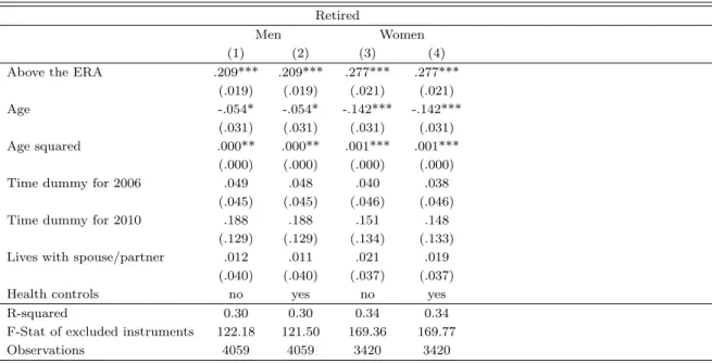
Almost 23% (816 individuals) of the individuals working at baseline retired between 2004 and 2010. Among them, 45% (365 individuals) had reached the national ERA during the same period. It suggests that actual retirement behaviour is well correlated with the ERA. First stage results are reported in Table 8 for men and women respectively. As expected, they indicate that the ERA is an important predictor of retirement. Reaching the ERA increases the probability of retiring by 21 and 28 percentage points for men and women respectively (both effects are significant at the 1% level). These results, combined with F-stats on excluded instruments of 122.2 and 169.4 for men and women respectively, show that reaching the ERA provides an strong exogeneous shock on retirement behaviour. Once controlling for these country-specific age breaks, the probability of retiring decreases with age up to a certain point, where it increases again – probably when reaching the official retirement age. Finally, neither time dummies for 2006 and 2010 nor marital status appear to be statistically important for retirement behaviour.
4.2 The impact of retirement on BMI, overweight and obesity
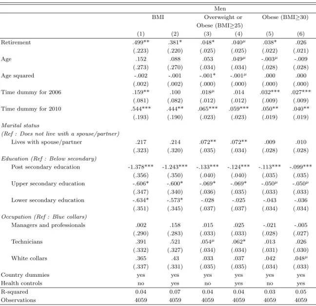
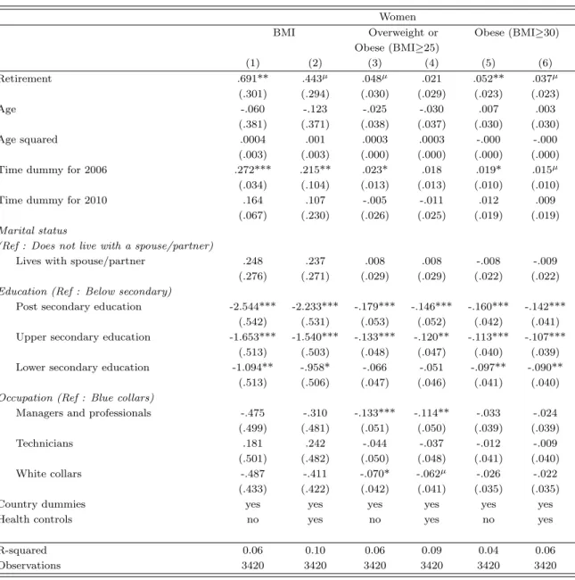
Given the differences in terms of both biological consititutions and labour market histories, we run separate models for men and women. Tables 4 and 5 report the POLS estimates for the BMI (columns 1 and 2), the probability of being either overweight or obese (columns 3 and 4) and the probability of being obese (columns 5 and 6) for men and women respectively. All specifications include age, age squared, time dummies for 2006 and 2010, marital status and time-invariant variables such as education, occupation and country dummies. The first column of each pair presents the results without including health controls, while the second column presents the results once controlling for self-rated health and the EURO-D depression index.
Most of the control variables are statistically significant and of the expected sign. A steep ed-ucation gradient in BMI, overweight and obesity is found for women and to a lower extent for men. Post-secondary education is indeed associated with a lower BMI and a lower probability of being either overweight or obese as well as being obese for both men and women. Once controlling for education, occupation is not significantly associated with BMI, overweight and obesity, except for women : females in managerial or professional occupations have a lower probability of being overweight than blue-collar females. Living with a spouse or partner does not seem to be correlated with BMI or the probability of being obese but is associated with a higher risk of being either overweight or obese among men. Most country indicators are significant.16 Surprisingly enough, once we control for retirement behaviour, age has a small and insignificant impact on BMI, overweight and obesity.
Our baseline specification reveals a positive and significant association between retirement and weight outcomes for men as well as women. Retirement is positively correlated with BMI : it increases BMI by 0.50 and 0.69 units for men and women respectively (both ef-fects are significant at the 5% level).17 It also increases men’s probability of being either overweight or obese and men’s probability of being obese by 4.8 and 3.8 percentage points respectively (both effects are significant at the 10% level). These coefficients correspond to a 7% (resp. 22%) increase in the probability of being overweight or obese (resp. obese) for men (compared with the sample average). Retirement also increase women’s probability of being obese by 5.2 percentage points (at the 5% significance level). It represents a 37% increase in the probability of being obese for women. Results go in the same direction once controlling for health variables, although the magnitude of the effects declines and most results become only marginally significant. Once controlling for health variables, retirement among men becomes only marginally associated with the probability of being either overweight or obese. However, it leads to a modest weight gain (0.38 BMI gain on average, at the 10% significance level). As for women, retirement becomes only marginally associated with BMI and the risk of obesity.
However, these correlations are hard to interpret, because they potentially reflect the
16
Results not shown but available upon request. 17
For an average man measuring 1.75m and weighing 82kg, it corresponds to a 1.5 kilo gain. As for an average woman measuring 1.63m and weighing 69kg, it corresponds to a 1.8 kilo gain.
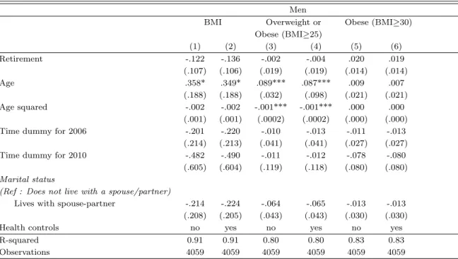
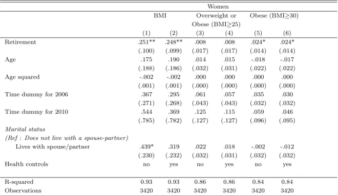
effects of unobserved characteristics that may affect both weight outcomes and retirement behaviour. The importance of confounding factors is apparent when we look at the coefficents on retirement once implementing fixed-effect regressions (see Table 6 and Table 7 for men and women respectively). Once taken into account the potential endogeneity arising from the correlation between retirement and time-invariant unobserved characteristics, retirement is no longer significantly associated with weight outcomes for men. The sign of the coefficient even becomes negative for BMI and the probability of being either overweight or obese (al-though both effects are insignificant at conventional levels). Conversely, retirement leads to weight gain (by 0.25 BMI, at the 5% significance level) and increases the probability of being obese for women (at the 10% significance level), although the magnitude of the estimates declines as compared to POLS results. Not controlling for time-invariant factors – such as time preference for instance, which has a positive effect both on the probability of retiring and on weight gain – may indeed generate an upward bias and account for the larger effect of retirement on weight in POLS models. Controlling for health variables only marginally affects the estimates, suggesting that time-invariant health characteristics affect weight out-comes to a larger extent than health changes over time.
However, the fixed-effect estimates cannot be interpreted as causal : a number of omitted time-varying factors can easily generate some bias in the results. Health or psychological deteriorations – for instance – may trigger both retirement and weight change. Hence, we need to take into account the remaining endogeneity in the model by instrumenting retire-ment behaviour. Results are presented in Tables 9 and 10 for men and women respectively. Under the hypothesis that reaching the ERA is a valid instrument, our preferred IV estimates show that retirement induced by discontinuous incentives in early retirement schemes causes a 13 percentage point increase in the probability of being obese (at the 5% level) within a two to four-year period among men. It corresponds to a 60% increase in the probability of being obese within a two to four-year period. However, it does not significantly affect men’s BMI nor men’s probability of being either overweight or obese, although both coefficients are positive.18 Our results thus suggest a non linear impact of retirement on men’s BMI : retirement would mostly affect the right-hand side of the BMI distribution.
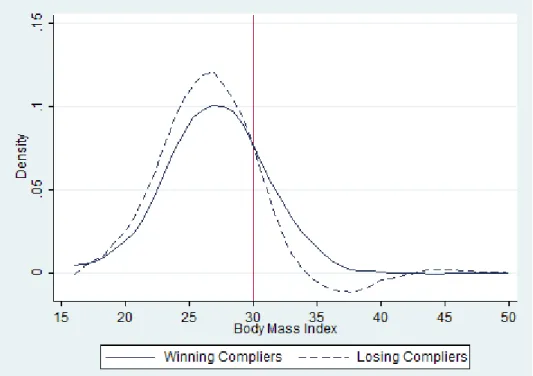
To inquire this further, we estimate the distribution of the BMI under different treatments for the subpopulation of compliers, following Imbens and Rubin (1997b).19 Figure 3 plots the estimated BMI distributions for winning and losing compliers. In our setup, winning compli-ers are individuals who became eligible to early retirement schemes between two subsequent
18The coefficients associated with the effect of retirement on BMI in FEIV models are very close to the ones obtained for the USA using a similar FEIV strategy. We find that retirement causes a 0.47 and 0.18 BMI increase within a two to four-year period among men and women respectively (although both coefficients are insignificant at conventional levels). These estimates are comparable to Chung et al. (2009) findings : on US data, retirement causes a 0.24 increase in BMI within a two-year period (at the 10% significance level). Unfortunately, as Chung et al. (2009) did not study the causal impact of retirement on the probability of being either overweight or obese nor on the probability of being obese, other comparisons based on the magnitude of the coefficients cannot be made.
19
waves of the survey and did retire then; losing compliers are individuals whose eligibility to early retirement schemes as well as retirement status did not change between two subsequent waves of the survey. According to Figure 3, the density fonction of winning compliers is shifted to the right compared to losing compliers. Winning compliers also seem to be more dispersed than losing compliers. Interestingly, the right tail of the winning compliers’ density is fatter after threshold 30. This is evidence that obese individuals are more frequent among the winning compliers. This piece of graphical evidence is consistent with the IV results discussed above and the idea that retirement has a non-linear impact on men’s BMI.
Overall, retirement seems to have a non-linear impact on men’s BMI and mostly affects the right-hand side of the BMI distribution, i.e, after threshold 30. As for women, Table 10 shows that they do not experience weight changes following retirement. The coefficient associated with retirement is never significant, whatever the outcome.
4.3 Heterogeneous effects of retirement
The impact of retirement on weight outcomes is likely to be highly heterogeneous across job types. In particular, individuals having retired from physically-demanding jobs are likely to gain weight if they do not compensate the direct reduction in job-related exercise by in-creasing their leisure-time physical activity or by dein-creasing their food intake. In order to test for this, we re-run our FEIV models by adding an interaction term of retirement sta-tus with a measure of previous job’s physical strenuousness. The physical strenuousness of work is measured using a question asking workers their opinion about the following state-ment : “My job is physically demanding”. Four answers are available ranging from “strongly agree” to “strongly disagree”. We dichotomise the responses into strenous work (strongly agree/agree) and sedentary work (disagree/strongly disagree). As this information is only available in SHARE for individuals who were working at baseline, FEIV models are estimated on a smaller sample – 934 men and 808 women across three waves. Among these individuals working at baseline, 56.4% had a sedentary job and 43.6% had a strenuous job. Table 11 shows the results when interacting retirement status with our indicator of job strenuous-ness.20 As controlling for health variables has little to no effect on FEIV estimates, Table 11
reports the FEIV estimates for the BMI (columns 1 and 2), the probability of being either overweight or obese (columns 3 and 4) and the probability of being obese (columns 5 and 6) for the baseline specification only. The first column of each pair presents the results for men, while the second column presents the results for women. As shown in column (5), the retirement effect on obesity seems to be mainly driven by men having retired from strenuous jobs. The coefficient associated with retirement is equal to 0.16 and insignificant at conven-tional levels, but the interaction term is equal to 0.10 and significant at the 5% level. Both coefficients are jointly significant at the 5% level. Overall, retirement causes a 26 percentage point increase in the probability of being obese among men having retired from strenuous jobs within two to four-year period (at the 5% significance level). This result is robust to the threshold chosen for obesity : among men having retired from strenuous jobs, retirement
significantly increases the probability of having a BMI above 31 (the interaction term is sig-nificant at the 5% level).21 Conversely, retirement does not seem to have a significant impact on neither the BMI, the probability of being either overweight or obese nor the probability of being obese among men having retired from sedentary occupations. Overall, our results suggest that retiring from a strenuous job has a triggering effect on obesity for men. As for women, columns (2), (4) and (6) show that they do not experience weight changes following retirement, whether they had retired from strenuous or sedentary jobs. The coefficients asso-ciated with the retirement indicator and the interaction term are never significant, whatever the outcome.
The impact of retirement on weight outcomes is also likely to be highly heterogeneous across weight categories at baseline. Additional results show that the causal impact of re-tirement on the probability of being obese is only significant for men who already had a BMI higher than 24 at baseline. This result holds for both specifications (with and without the interaction term retirement*job strenuousness22). The “marginal” individual is thus likely to be a man already overweight or not far from the overweight threshold, i.e, at risk of obesity. Overall, our results show retirement effects can be highly heterogeneous : in particular, retiring from a strenuous job has a triggering effect on obesity for men already at risk of obesity.
4.4 Underlying mechanisms
In this paragraph, we further investigate the heterogeneous response to retirement according to gender. As retirement is likely to operate on weight through physical activity and food intake, we try to assess whether changes in food intake and physical activity following re-tirement are gender-specific. Due to data limitations23, we focus on changes in leisure-time
21
The coefficient associated with retirement is equal to 0.06 (standard error : 0.09) and insignificant. The coefficient associated with the interaction term is equal to 0.10 (standard error : 0.05) and significant at the 5% level.
22
When considering men who already had a BMI higher than 24 at baseline, our sample goes down to 1054 individuals across the three waves. We re-run our FEIV models on this subsample to estimate the effect of retirement on the probability of being obese. The coefficient associated with retirement is equal to 0.15 (standard error : 0.07) and significant the 5% level. The coefficient associated with retirement is insignificant on the subsample of men who had a BMI lower than 24 at baseline. We also re-run our FEIV models including the interaction term retirement status*job strenuousness. When considering men who already had a BMI higher than 24 and who were working at baseline, our sample goes down to 721 individuals across the three waves. When estimating the effect of retirement on obesity, the coefficient associated with retirement is equal to 0.17 (standard error : 0.14) and insignificant at conventional levels. The coefficient associated with the interaction term is equal to 0.11 (standard error : 0.06) and significant at the 10% level. Both coefficients are insignificant on the subsample of men who had a BMI lower than 24 and who were working at baseline.
23SHARE contains two measures of food consumption : the monthly household expenditure on food con-sumed away from home and the monthly household expenditure on food concon-sumed at home. However, these two measures are hard to interpret : they are likely to reflect a household joint decision concerning food consumption. They do not necessarily reflect an individual change in food consumption – and even less an individual change in food intake.
physical activity after retirement. Leisure-time physical activity is captured in SHARE by the following question : “How often do you engage in activities that require a moderate level of energy such as gardening, cleaning the car, or doing a walk?”. Four answers are available ranging from “more than once a week” to “hardly ever, or never”. We dichotomize the responses into high (more than once a week/once a week) and low moderate leisure-time physical activity (one to three times a month/hardly ever, or never). Our FEIV models show that women tend to increase their leisure-time physical activity following retirement while men do not. Retirement causes a 14 percentage point increase in the probability of perform-ing a moderate physical activity at least once a week (at the 5% significance level) among women. The corresponding figure for men is equal to 7 percentage points and insignificant at conventional levels. This would be suggestive evidence that the heterogeneous impact of retirement across genders is partly explained by women’s higher propensity to engage in leisure-time physical activities following retirement. However, the results do not seem robust to alternative dichotomisations of leisure-time physical activity. When using an alternative dichotomisation of leisure-time physical activity (hardly never or never versus more than once a week/once a week/one to three times a month), we find that retirement causes a 11 (12) percentage point increase in the probability of performing a moderate physical activity at least one to three times a month among men (women). Both coefficients are significant at the 5% significance level.
Overall, our data lead to inconclusive results with regard to gender-specific patterns in leisure-time physical activity following retirement. Moreover, only very precise measures of physical activity – both at work and during leisure time – would have allowed us to investigate whether individuals actually compensate the direct reduction in job-related exercise by in-creasing their leisure-time physical activity following retirement. Thus, data limitations make it difficult to explore the underlying mechanisms through which retirement affects weight as well as the gender-specific patterns in food intake and physical activity.
4.5 Robustness checks
Our estimation strategy is likely to yield unbiased results if properly controlling for the age trend. As one may worry that our results be driven by an inadequate estimation of the age effect, we have tried linear, quadratic (presented) and quartic age terms in robustness checks. Results are qualitatively similar.24
As underweight status is associated with a higher risk of morbidity and mortality for the elderly (Corrada et al. (2006)), one could be afraid that underweight individuals have a different response to retirement. It might be the case that underweight individuals lose
24
When introducing age as a linear term, the point estimate associated with the effect of retirement on the probability of being obese in FEIV moldels for men is very similar to the one obtained when introducing age as a quadratic term (presented). The coefficient associated with retirement is equal to 0.13 (standard error : 0.06) and significant at the 5% level. The corresponding figure when introducing age as a quartic term is 0.14 (standard error : 0.08), significant at the 10% level. We find no significant results for men’s BMI nor men’s probability of being either overweight or obese. No significant results are found for women.
weight because of retirement, thus leading to an overall insignificant impact of retirement on BMI. We check that our results are robust to the exclusion of underweight individuals by re-running our IV estimates on normal, overweight and obese individuals at baseline. Results are virtually unchanged.25
Up until now, retirement was defined using a question on self-declared current job situation (see Data section). According to this definition, anyone who declares herself to be retired is considered as retired. One concern could be that individuals declare themselves as retired even when working full or part-time, simply because they have left their “career” job. We use an alternative definition according to which anyone who is in the paid labour force is considered as employed (see Data section). Results from the FEIV regressions using this alternative definition show that the point estimate of the retirement indicator is very similar to those presented in Table 9 and marginally significant at the 15% level.26 Given that only 395 individuals retire between 2004 and 2010 according to this alternative definition, this result is likely to be due to a power problem.
An additional concern is that there might be other things than retirement at ERAs that could cause a nonlinear relationship between weight and age at these given ages. For example, one may think of country-specific cohort effects which may reflect differencial trends in food supplies, health policies or early life conditions. An imperfect way to test for this is to introduce the age*country and age2*country terms in our FEIV models to test whether age has a differential impact on weight across countries. All coefficients associated with these additional terms are insignificant in all our FEIV models. The point estimates obtained on the retirement indicator do not significantly vary as compared to those presented in Table 9. In particular, when considering the probability of being obese as an outcome, the coefficient associated with retirement in the FEIV model for men is equal to 0.14 (standard error : 0.15) and significant at the 10% level.
Finally, we conduct a placebo test to back the reliance of our results. We evaluate the impact of a fictive state of the world where ERAs would be interchanged across countries.27 We re-run our FEIV regressions with this fictive instrument. As expected, the coefficient associated with this fictive instrument in the first stage is close to 0 and non significant at conventional levels. The F-stat of excluded instrument is equal to 2.24 – below the standard requirement of 10 (Bound et al. (1995)) – thus suggesting a weak instrument problem. When considering the probability of being obese as an outcome, the coefficient associated with retirement in
25When considering the probability of being obese as the outcome in the FEIV model for men, the coefficient associated with retirement is equal to 0.13 (standard error : 0.06) and significant at the 5% level. When considering either the BMI or the probability of being obese as the outcome, the coefficient associated with the retirement indicator in FEIV models for men is still insignificant. No significant results are found for women.
26
When considering the probability of being obese as the outcome in the FEIV model for men, the coefficient associated with retirement is equal to 0.13 (standard error : 0.09) and marginally significant at the 15% level. We find no significant results for men’s BMI nor men’s probability of being either overweight or obese. No significant results are found for women.
27The design of the placebo reform is as following : we assign to each country a fictive ERA. For instance, France’s ERA is set to 61. The corresponding ERAs for Germany, Sweden, Switzerland, Spain, Austria, Italy and Belgium are 57, 60, 60, 63, 59, 62 and 62, respectively.
the FEIV model for men is equal to 0.09 (standard error : 0.43) and non significant at conventional levels (p-value : 0.84).
5
Conclusion
This paper studies the effect of retirement on several weight outcomes using the 2004, 2006 and 2010 waves of SHARE. It exploits the European variation in ERAs and the stepwise in-crease in ERAs in Austria and Italy to produce an exogeneous shock on retirement behaviour. This allows us to estimate the short-term causal impact of retirement on weight. Our results show that retirement induced by social security rules causes a 13 percentage point increase in the probability of being obese within a two to four-year period among 50-69 year-old men. Our findings suggest that retirement has a non-linear impact on men’s BMI, mostly affecting the right-hand side of the distribution. We give evidence that this effect is highly heteroge-neous and driven by men having retired from strenuous jobs and who were already at risk of obesity. No significant effects are found among women.
A possible interpretation of our findings is that the impact of retirement on weight is likely to be driven by a direct reduction in job-related exercise. The gender-heterogeneity of our results is likely to be explained by gender-specific patterns in food intake and physical activity following retirement. There is some evidence in the literature that women adjust to retirement more sucessfully than men (Barnes and Parry (2004)). Women would adjust their food diet and physical activity to a better extent than men, thus compensating the reduction in job-related exercise following retirement. Due to data limitations, we were not able to investigate these gender-specific patterns in greater detail.
Our findings are consistent with a more and more common interpretation of the results of the literature focusing on the link between retirement and health. Retirement is likely to reduce the amount of stress and physical strain that an individual experiences from work, and may thus positively affect subjective dimensions of health. As retirement is also likely to reduce the amount of physical activity and mentally stimulating activities after retirement, it may at the same time negatively affect objective dimensions of health. Retirement has indeed been shown to deteriorate physical dimensions of health (such as cognitive function-ing or cardiovascular diseases), and improve subjective dimensions of health at the same time (such as self-rated health or mental health).28 Our results are highly consistent with this interpretation, as the BMI can be seen as an objective measure of health, likely to be measured and known to the respondent himself. The direct reduction in job-related exercise following retirement is likely to deteriorate this specific dimension of health, along with other dimensions of objective health.
28
Although some findings in the literature are not consistent with this interpretation. See for instance Dave et al. (2006), who find negative effects of retirement on both objective and subjective measures on health or Coe and Zamarro (2011), who find positive effects on both objective and subjective measures on health.
Finally, our results have some important policy implications. Given the increasing number of people approaching retirement age and the upward trend in obesity rates (where each cohort is heavier than the previous one), men retiring from strenuous jobs in the near future will be likely to suffer from health disorders following retirement. Public health policies specifically targeted at this population should be considered in order to guarantee healthy ageing and healthy life years following retirement.
Bibliography
Anderson, L. and J. Mellor (2008): “Predicting health behaviors with an experimental measure of risk preference,” Journal of Health Economics, 27, 1260–1274.
Andreyeva, T., P. Michaud, and A. Van Soest (2007): “Obesity and health in Euro-peans aged 50 years and older,” Public Health, 121, 497–509.
Angrist, J., G. Imbens, and D. Rubin (1996): “Identification of causal effects using instrumental variables,” Journal of the American statistical Association, 91, 444–455. Barnes, H. and J. Parry (2004): “Renegotiating identity and relationships: Men and
women’s adjustments to retirement,” Ageing and Society, 24, 213–233.
Behncke, S. (2011): “Does retirement trigger ill health?” Health Economics, 21, 282–300. Blake, H. and C. Garrouste (2012): “Collateral effects of a pension reform in France,”
Tech. rep., Health, Econometrics and Data Group (HEDG) Working Papers 12/16, HEDG, c/o Department of Economics, University of York.
B¨ockerman, P., E. Johansson, P. Jousilahti, and A. Uutela (2008): “The physical strenuousness of work is slightly associated with an upward trend in the BMI,” Social Science & Medicine, 66, 1346–1355.
Bonsang, E., S. Adam, and S. Perelman (2012): “Does retirement affect cognitive functioning?” Journal of health economics, 31, 490–501.
Bound, J., D. A. Jaeger, and R. M. Baker (1995): “Problems with instrumental variables estimation when the correlation between the instruments and the endogenous explanatory variable is weak,” Journal of the American statistical association, 90, 443– 450.
Bradford, L. (1979): “Can You Survive Your Retirement?” Harvard Business Review, 57, 103–109.
Brunello, G. and B. d’Hombres (2007): “Does body weight affect wages? Evidence from Europe,” Economics & Human Biology, 5, 1–19.
Brunello, G., D. Fabbri, and M. Fort (2013): “The causal effect of education on body mass: Evidence from Europe,” Journal of Labor Economics, 31, 195–223.
Burkhauser, R. and J. Cawley (2006): “The importance of objective health measures in predicting early receipt of social security benefits: The case of fatness,” Tech. rep., Michigan Retirement Research Center Working Papers 148, University of Michigan.
——— (2008): “Beyond BMI: The value of more accurate measures of fatness and obesity in social science research,” Journal of Health Economics, 27, 519–529.
Cawley, J. (2004): “The impact of obesity on wages,” Journal of Human Resources, 39, 451–474.
Cawley, J., J. Moran, and K. Simon (2010): “The impact of income on the weight of elderly Americans,” Health Economics, 19, 979–993.
Charles, K. (2004): “Is retirement depressing?: Labor force inactivity and psychological well-being in later life,” Research in Labor Economics, 23, 269–299.
Chung, S., M. Domino, and S. Stearns (2009): “The effect of retirement on weight,” The Journals of Gerontology Series B: Psychological Sciences and Social Sciences, 64, 656–665. Chung, S., B. Popkin, M. Domino, and S. Stearns (2007): “Effect of Retirement on Eating Out and Weight Change: An Analysis of Gender Differences,” Obesity, 15, 1053– 1060.
Coe, N. and M. Lindeboom (2008): “Does retirement kill you? Evidence from early re-tirement windows,” Tech. rep.
Coe, N. and G. Zamarro (2011): “Retirement effects on health in Europe,” Journal of Health Economics, 30, 77–86.
Colchero, M., B. Caballero, and D. Bishai (2008): “The effect of income and occu-pation on body mass index among women in the Cebu Longitudinal Health and Nutrition Surveys (1983-2002),” Social Science & Medicine, 66, 1967–1978.
Corrada, M., C. Kawas, F. Mozaffar, and A. Paganini-Hill (2006): “Association of body mass index and weight change with all-cause mortality in the elderly,” American Journal of Epidemiology, 163, 938–949.
Dave, D., I. Rashad, and J. Spasojevic (2006): “The effects of retirement on physical and mental health outcomes,” Tech. rep., NBER Working Paper No. 12123.
De Luca, G. (2009): “Determinants of the attrition process in the first two waves of SHARE,” Tech. rep., mimeo.
Eibich, P. (2014): “Understanding the effect of retirement on health using Regression Dis-continuity Design,” Tech. rep., mimeo.
Emery, C., J. Dinet, A. Lafuma, C. Sermet, B. Khoshnood, and F. Fagnani (2007): “ ´Evaluation du coˆut associ´e `a l’ob´esit´e en France,” La Presse M´edicale, 36, 832–840. Finkelstein, E., I. Fiebelkorn, and G. Wang (2003): “National medical spending
attributable to overweight and obesity: how much, and who’s paying?” Health Affairs, 22, 3–219.
Forman-Hoffman, V., K. Richardson, J. Yankey, S. Hillis, R. Wallace, and F. Wolinsky (2008): “Retirement and weight changes among men and women in the
Health and Retirement Study,” The Journals of Gerontology Series B: Psychological Sci-ences and Social SciSci-ences, 63, 146–153.
Friedmann, E. and R. Havighurst (1954): The meaning of work and retirement, Univer-sity of Chicago Press, Chicago.
Goldman, D., D. Lakdawalla, and Y. Zheng (2008): “Retirement and Weight,” Tech. rep., mimeo.
Grossman, M. (1972): “On the concept of health capital and the demand for health,” The Journal of Political Economy, 80, 223–255.
Gruber, J. and D. Wise (1999): Social Security and Retirement around the World., Uni-versity of Chicago Press, Chicago.
Gueorguieva, R., J. Sindelar, R. Wu, and W. Gallo (2010): “Differential changes in body mass index after retirement by occupation: hierarchical models,” International Journal of Public Health, 56, 111–116.
Gustman, A. L. and T. Steinmeier (2009): “Integrating retirement models,” Tech. rep., NBER Working Paper No. 15607.
Hurst, E. (2008): “The retirement of a consumption puzzle,” Tech. rep., National Bureau of Economic Research (NBER) Working papers 13789.
IASO/IOTF (2002): “Obesity in Europe. The Case for Action.” Available at http://www.iaso.org/site_media/uploads/Sep_2002_Obesity_in_Europe_Case_ for_Action_2002.pdf.
——— (2010): “Obesity and overweight,” Available at http://www.iaso.org/iotf/ obesity/obesitytheglobalepidemic/.
Ikeda, S., M. Kang, and F. Ohtake (2010): “Hyperbolic discounting, the sign effect, and the body mass index,” Journal of Health Economics, 29, 268–284.
Imbens, G. W. and J. D. Angrist (1994): “Identification and estimation of local average treatment effects,” Econometrica, 62, 467–476.
Imbens, G. W. and D. B. Rubin (1997a): “Bayesian inference for causal effects in ran-domized experiments with noncompliance,” Annals of Statistics, 25, 305–327.
——— (1997b): “Estimating outcome distributions for compliers in instrumental variables models,” The Review of Economic Studies, 64, 555–574.
Keese, M. (2006): Live longer, work longer, Paris, OECD.
Lallukka, T., E. Lahelma, O. Rahkonen, E. Roos, E. Laaksonen, P. Martikainen, J. Head, E. Brunner, A. Mosdol, M. Marmot, et al. (2008a): “Associations of job strain and working overtime with adverse health behaviors and obesity: evidence from the
Whitehall II Study, Helsinki Health Study, and the Japanese Civil Servants Study,” Social Science & Medicine, 66, 1681–1698.
Lallukka, T., S. Sarlio-L¨ahteenkorva, L. Kaila-Kangas, J. Pitk¨aniemi, R. Luukkonen, and P. Leino-Arjas (2008b): “Working conditions and weight gain: a 28-year follow-up study of industrial employees,” European Journal of Epidemiology, 23, 303–310.
Manoli, D. and A. Weber (2012): “The Effects of Increasing the Early Retirement Age on Social Security Claims and Job Exits,” Tech. rep., mimeo.
Marcus, J. (2012): “Does job loss make you smoke and gain weight?” Tech. rep.
Morris, S. (2006): “Body mass index and occupational attainment,” Journal of Health Economics, 25, 347–364.
Muenster, E., H. Rueger, E. Ochsmann, S. Letzel, and A. Toschke (2011): “Asso-ciation between overweight, obesity and self-perceived job insecurity in German employees,” BMC public health, 11, 162.
Must, A., J. Spadano, E. Coakley, A. Field, G. Colditz, and W. Dietz (1999): “The disease burden associated with overweight and obesity,” JAMA: the Journal of the American Medical Association, 282, 1523–1529.
Neuman, K. (2008): “Quit your job and get healthier? The effect of retirement on health,” Journal of Labor Research, 29, 177–201.
Niedhammer, I., I. Bugel, S. Bonenfant, M. Goldberg, and A. Leclere (2000): “Validity of self-reported weight and height in the French GAZEL cohort,” International Journal of Obesity, 24, 1111–1118.
Nooyens, A., T. Visscher, A. Schuit, C. Van Rossum, W. Verschuren,
W. Van Mechelen, and J. Seidell (2005): “Effects of retirement on lifestyle in re-lation to changes in weight and waist circumference in Dutch men: a prospective study,” Public Health Nutrition, 8, 1266–1274.
OECD (2010): Health at a glance: Europe 2010, Paris, OECD.
——— (2011): Pensions at a Glance 2011 : Retirement-Income Systems in OECD and G20 Countries, Paris, OECD, available at www.oecd.org/els/social/pensions/PAG.
Peytremann-Bridevaux, I. and B. Santos-Eggimann (2008): “Health correlates of overweight and obesity in adults aged 50 years and over: results from the Survey of Health, Ageing and Retirement in Europe (SHARE),” Swiss Medical Weekly, 138, 261–266. Prentice, A. and S. Jebb (2001): “Beyond body mass index,” Obesity Reviews, 2, 141–147.