HAL Id: hal-01098040
https://hal.inria.fr/hal-01098040
Preprint submitted on 14 Feb 2019
HAL is a multi-disciplinary open access
archive for the deposit and dissemination of
sci-entific research documents, whether they are
pub-lished or not. The documents may come from
teaching and research institutions in France or
abroad, or from public or private research centers.
L’archive ouverte pluridisciplinaire HAL, est
destinée au dépôt et à la diffusion de documents
scientifiques de niveau recherche, publiés ou non,
émanant des établissements d’enseignement et de
recherche français ou étrangers, des laboratoires
publics ou privés.
Distributed under a Creative Commons Attribution - NonCommercial - NoDerivatives| 4.0
Feature learning for multi-task inverse reinforcement
learning
Olivier Mangin, Pierre-Yves Ouedeyer
To cite this version:
Olivier Mangin, Pierre-Yves Ouedeyer. Feature learning for multi-task inverse reinforcement learning.
2014. �hal-01098040�
Feature learning for multi-task inverse
reinforcement learning
Olivier Mangin and Pierre-Yves Ouedeyer
December 22, 2014
Abstract
In this paper we study the question of life long learning of behaviors from human demonstrations by an intelligent system. One approach is to model the observed demonstrations by a stationary policy. Inverse rein-forcement learning, on the other hand, searches a reward function that makes the observed policy closed to optimal in the corresponding Markov decision process. This approach provides a model of the task solved by the demonstrator and has been shown to lead to better generalization in un-known contexts. However both approaches focus on learning a single task from the expert demonstration. In this paper we propose a feature learn-ing approach for inverse reinforcement learnlearn-ing in which several different tasks are demonstrated, but in which each task is modeled as a mixture of several, simpler, primitive tasks. We present an algorithm based on an al-ternate gradient descent to learn simultaneously a dictionary of primitive tasks (in the form of reward functions) and their combination into an ap-proximation of the task underlying observed behavior. We illustrate how this approach enables efficient re-use of knowledge from previous demon-strations. Namely knowledge on tasks that were previously observed by the learner is used to improve the learning of a new composite behavior, thus achieving transfer of knowledge between tasks.
1
Introduction
Understanding and imitating human behaviors is a key capability for robots to collaborate with humans or even to be accepted in their living environments. However human behaviors feature a huge variety both in their nature and their complexity. Many approaches to the problems of human behavior understand-ing and learnunderstand-ing from demonstration focus on directly mimickunderstand-ing the observed behavior. In that context, the human behavior is often represented as a map-ping from time to actions or a stationary policy, that is to say a mapmap-ping from states of the agent and its environment to a probability distribution over possi-ble actions. However the policy space is generally very large and representing a behavior as a sequence of actions, without regularization, might not be robust to changes in the context. For example, for the task of grasping an object, if
the hand starting position or the object position changes, the motion to grasp it will look very different. For a well chosen representation of the state, learn-ing a policy may address this issue. However for rich state representations, the demonstrator policy is often only observed in a small subset of the state space which might lead to poor generalisation. Previous work in inverse reinforcement
learning (IRL) [Ng and Russell,2000,Abbeel and Ng,2004,Neu and Szepesv´ari,
2007] has shown that it can provide better generalization of the learnt behaviors
to new unobserved contexts, to learn a model of the task solved by the demon-strator. More precisely, the learner assumes that the demonstrator’s intention is to solve a task, it then tries to solve the same task instead of directly mim-icking the demonstrator’s actions. Furthermore inverse reinforcement learning
or similarly inverse optimal control [Ratliff et al., 2006] also has the advantage
of providing a model of the demonstrator’s intention, which we often denote as task in this paper.
However inverse reinforcement techniques have mainly been studied in the single task setup, where appropriate features are provided, whereas an important challenge for life long learning systems is to be able to efficiently re-use previous knowledge to understand new situations, which is an aspect of transfer learning
as stated bySilver et al.[2013]. For example a child learning to play a new ball
game won’t learn again how to grasp a ball, how to throw it and how to run. While observing a demonstration of the new game the child would not focus on every position of each body joint along the demonstration but rather recognize a set of basic behaviors, e.g. running to a point while keeping the ball in hands and then throwing the ball to an other position. Therefore, an approach that represents the new activity in terms of known primitive tasks, eventually learn-ing some new misslearn-ing parts, rather than learnlearn-ing everythlearn-ing from scratch would provide a better model of the graceful increase in the complexity of achievable tasks that is observed on children.
The idea of learning a dictionary whose elements can be combined to ap-proximate observations, denoted as dictionary learning, has been largely studied
in the machine learning community where it lead to good results [Aharon et al.,
2005, Lee and Seung, 1999]. Typically, inverse reinforcement learning is de-scribed as learning a single task from an expert, which, for non-trivial models of states and actions, requires a huge number of demonstrations. In order to make the number of required demonstrations feasible, one often uses adequate features to reduce the search space. However specifying good features requires prior knowledge about the task and learning the features for one task requires a lot of demonstrations of one single task. Being able to learn a dictionary of features from several related but different tasks can reduce the amount of demonstrations required for each task which would open new applications for inverse reinforcement learning such as recognizing simple actions, as grasping or throwing the ball in the ball game example by observing people playing, with-out requiring an expert to provide many demonstration of the “throwing a ball” primitive action.
In this paper we therefore focus on the question of how to represent demon-strated behaviors as the combination of simpler primitive behaviors that can be
re-used in other contexts. We present an algorithm that, by observing demon-strations of an expert solving multiple tasks, learns a dictionary of primitive behaviors and combine them to account for the observations. We demonstrate how such an approach can be beneficial for life long learning capabilities in a simple toy experiment.
2
Related work
Inverse reinforcement learning algorithms takes as input demonstrations from an expert, more precisely trajectories in a Markov decision process (MDP). It is generally assumed that a model of the transition is known and that the expert is acting optimally or close to optimally with respect to an unknown reward function. The goal of inverse reinforcement learning is then to find a reward for which the expert behavior is optimal. It is however well known that this problem is ill-posed: nonnegative scaling of reward and addition of a potential
function does not change the optimality of policies [Ng et al.,1999] and for non
trivial problems a lot more solutions may exist.
Since the seminal work from Ng and Russell[2000] introduced the problem
of inverse reinforcement learning, many algorithms have been proposed to solve it [Abbeel and Ng, 2004, Ratliff et al., 2006, Ramachandran and Amir, 2007, Ziebart et al.,2008,Neu and Szepesv´ari,2007].
More recent work also address other aspects of inverse reinforcement learning
that makes it more relevant to life long learning. Levine et al. [2010] introduce
an algorithm to both learn an estimate of the reward optimized by the expert and features to efficiently represent it. They also demonstrate how the learned
features can be transfered to a new environment. Jetchev and Toussaint[2011]
present an inverse feedback learning approach to a grasping problem. They demonstrated how enforcing sparsity of the feedback function (conceptually equivalent to a reward function) can also solve a task space retrieval problem.
While in the works presented above the expert only demonstrates a single
task, Babes-Vroman et al.[2011] present an EM-based algorithm which, from
unlabeled demonstrations of several tasks, infer a clustering of these
demon-strations together with a set of models. Almingol et al. [2013] also recently
developed similar ideas.
The algorithm presented in this paper extends the gradient approach by Neu and Szepesv´ari [2007] to learn a dictionary of primitive reward functions that can be combined together to model the intention of the expert in each
demonstration. Our work is different from the one proposed byBabes-Vroman
et al.[2011] since it not only learns from demonstrations of several tasks but also enable transfer of the knowledge from one task to an other. It thus includes ideas fromLevine et al.[2010] but extended to unlabeled multi-task demonstrations.
3
Algorithm
We assume that we observe demonstrations ξ from an expert, that are sequences
(xt, at) of states xt∈ X and action at∈ A, such that ξ = (xt, at)t∈[|1,T |].
A Markov decision process (MDP) is defined as a quintuple (X , A, γ, P, r) where γ is the discount factor. P , the transition probability, is a mapping from state actions pairs to probability distributions over next states. We denote by
P (x′|x, a) the probability to transition to state x′ from state x, knowing that
action a was taken. Finally, r : X × A → R is the reward function.
A stationary policy π is a mapping from states to probability densities over
actions. For a given MDP and a policy one can define the value function Vπ,
the action value function Qπ:
Vπ(x) = E ∞ t=0 γtr(Xt, At) X0= x (1) Qπ(x, a) = E ∞ t=0 γtr(Xt, At) X0= x, A0= a (2)
and the associated optimal value function V∗(x) = supπVπ(x), ∀x ∈ X and
op-timal action value function Q∗(x, a) = supπQπ(x, a), ∀(x, a) ∈ X ×A . A policy
that is optimal (w.r.t. to equation (1)) over all state is said to be optimal. Greedy
policies over Q∗, that is to say policies such that π(arg maxaQ∗(x, a)|x) = 1 ,
are known to be optimal. Finally Q∗is solution of the fixed point equation given
in equation (3) that provides an algorithm known as dynamic programming to
compute Q∗ for a known MDP.
Q∗(x, a) = r(x, a) + γ
y∈X
P (y|x, a) max
b∈AQ
∗(x, b) (3)
In the following we assume that the model of the world (i.e. states, actions and transitions) is fixed and that the discount factor γ is known. However we represent the intention of a demonstrator (called expert ) as acting optimally with respect to a task that is modelled as a reward function. Since the model of the world is fixed no distinction is made between a reward function r and the associated MDP, M DP (r).
3.1
Gradient for apprenticeship learning
In this section we present the algorithm and results introduced by Neu and
Szepesv´ari [2007]. For more details and proofs the reader is invited to look at the article.
Inverse reinforcement learning for apprenticeship learning is based in the assumption that the expert’s intention is to solve a task, modeled by a re-ward function. Mimicking the expert behavior therefore consists in using a
Szepesv´ari [2007] focuses on learning a reward such that an associated optimal policy matches the expert’s actions.
In this single task setup, the expert provides one or several demonstrations of solving the same task. The expert actions are modeled by a stationary policy
πE. The objective of apprenticeship learning becomes to find a policy π that
minimize the cost function from equation (4), in which µ denotes the average
state occupation, that is to say µE(x) = lim
T →∞Eπ 1 T T t=1 δXt=x . J (π) = x∈X ,a∈A µE(x)π(x|a) − πE(x|a) 2 (4)
For an expert demonstration represented by ξ = (xt, at)t∈[|1,T |]one estimates
J by equation (5), in which ˆµE,ξ and ˆπE,ξ are empirical estimates of µEand πE
from ξ.
Jξ(π) =
x∈X ,a∈A
ˆ
µE,ξ(x)π(x|a) − ˆπE,ξ(x|a)
2
(5)
In the following the reward rθ is parametrized by θ ∈ Θ where Θ ∈ Rd
and we denote by Q∗θthe optimal action value function of the MDP associated
to rθ. In practice linear features are used for r. Let G be a smooth mapping
from action value functions to policies that returns a close to greedy policy to
its argument. Instead of minimizing Jξ over any subset of policies, Neu and
Szepesv´ari [2007] suggests to constrain π to be of the form πθ= G(Q∗θ).
Solving the apprenticeship learning problem is then equivalent to finding θ that reaches:
min
θ∈ΘJξ(πθ) s.t. πθ= G(Q
∗
θ). (6)
In practice,Neu and Szepesv´ari[2007] uses Boltzmann policies as choice for
the G function, as given by equation (7) where the parameter β is a nonnegative real number. This choice ensures that G is infinitely differentiable. Assuming
that Q∗θ is differentiable w.r.t. θ its first derivate is given by equation (8).
G(Q)(a|x) = expβQ(x, a)
a′∈A expβQ(x, a′) (7) ∂G(Q∗θ)(a|x) ∂θk = G(Q∗θ)(a|x) ∂Q∗θ(x, a) ∂θk − a′∈A πθ(a′|x) ∂Q∗θ(x, a′) ∂θk (8)
The following proposition from Neu and Szepesv´ari [2007] provides both
guarantees that ∂Q
∗
θ(x, a)
∂θk
is meaningful and a practical way to compute it.
Proposition (Neu and Szepesvari). Assuming that rθ is differentiable w.r.t. θ
1. Q∗θ is uniformly Lipschitz-continuous as a function of θ in the sense that
there exist L′ > 0 such that for any (θ, θ′) ∈ Θ2, |Q∗θ(x, a) − Q∗θ(x, a)| ≤
L′∥θ − θ′∥
2. The gradient ∇θQ∗θ is defined almost everywhere
1 and is a solution of the
following fixed point equation, in which π is a greedy policy on Q∗
θ: φθ(x, a) = ∇θr(x, a) + γ y∈X P (y|x, a) b∈A π(b|y)φθ(y, b) (9)
The previous result thus provides an algorithm, similar to dynamic
pro-gramming that yields the derivative of Q∗θ with respect to θ. It it then easy
to combine it with the differentiates of Jξ with respect to π and G to obtain a
gradient descent algorithm that finds a local minima of the objective.
Neu and Szepesvari furthermore provides a variant of this algorithm follow-ing a natural gradient approach.
3.2
Feature learning for multi-task inverse reinforcement
learning (FactIRL)
In this section we extend the algorithm from Neu and Szepesv´ari [2007] to a
dictionary learning problem. We now assume that the expert provides several
demonstration of different but related tasks. The demonstrations are denoted ξi
with index i ∈ [|1, n|]. Each demonstration is modeled by a separate parameter
θ(i) that represents the tasks solved by the expert. We focus on a generative
model of mixtures of behaviors or tasks such that the combination of tasks can be represented as a reward function that is a linear combination of the reward functions of the mixed tasks.
More precisely, a matrix D ∈ Rd×k represents the dictionary and a matrix
H ∈ Rk×n the mixing coefficients. The columns of H are denoted h(i)such that
the parameters of the ith task are θ(i)= Dh(i).
In the following we present an algorithm that learns the matrix factorization that is to say the dictionary matrix D and associated coefficients H such that
θ(i)s are represented as combinations of k elements from a dictionary. The
algorithms minimizes the cumulated cost over all demonstrations denoted by
JΞ, where Ξ = (ξi)i∈[|1,n|], and defined in equation (10).
JΞ(D, H) = n i=1 Jξi(Dh (i)) (10)
In order to solve the problem arg minD,HJΞ(D, H) the algorithm alternates
steps that minimize the cost with respect to D, H being fixed, and with respect
to H, D being fixed. The second steps actually decomposes in n separate
problems similar to the one from previous section. Both steps uses a gradient descent approach where the gradients are given by eqs. (11) and (12).
∇DJΞ(D, H) = ∇θJξiDh (1) ... ∇θJξiDh (n) · HT (11) ∇HJΞ(D, H) = DT· ∇θJξiDh(1) ... ∇θJξiDh (n) (12) In practice the learner performs a fixed amount of gradient descent on each sub-problem (optimization of H and D), with Armijo step size adaptation be-fore switching to the other sub-problem. The algorithm stops when reaching convergence. It appears that this gradient descent algorithm is quite sensitive to initial conditions. A good empirical initialization of the dictionary is to first
learn θ(i)s with the flat approach, perform a PCA on the learnt parameters and
use it as an initial guess for the dictionary.2
4
Experiments
In these experiments a task refers to a MDP associated to a reward function. We consider composite tasks which means tasks that correspond to reward functions obtained by mixing several primitive reward functions.
The algorithm described above is experimented on a simple toy example
similar to the one from Neu and Szepesv´ari [2007]: a grid world (typically
of size 10 by 10) is considered in which actions corresponds to moves in four directions. Actions have the expected result, that is a displacement of one step in the expected direction, in 70% of the cases and results in a random move in the other cases; except when the requested move is not possible from current state (for example going up on top border) in which case the resulting move is drawn uniformly from feasible moves. The following uses a fixed discount factor γ = 0.9.
4.1
Validation
In a first experiment we compare our factorial algorithm to direct learning of the parameter representing a task with Neu and Szepesvari’s gradient (GradIRL), that we call flat learner to differentiate from the factorial approach.
More precisely a random dictionary of features is chosen, that is unknown from the apprentices, together with mixing coefficients that determine n distinct composite tasks. n experts are then used to generate demonstrations for each tasks (during training the expert may provide several demonstrations of each task).
The demonstrations obtained are fed to both flat and factorial apprentices. While the flat learners independently learn a model of each task, the factorial learner reconstructs a dictionary, shared amongst tasks together with mixing coefficients.
2Experiments presented further shows that the PCA strategy alone does not provide a good dictionary for our problem, but is an efficient initialization.
We evaluate the apprentices on each learnt task by measuring their average performance on the MDP corresponding to the demonstrated task, referred
as M DP (rreal). More precisely the apprentice can provide an optimal policy
πr∗learnt with respect to its model of the task, that is to say a policy optimal with
respect to the learnt reward rlearnt.3 This policy is then evaluated on the MDP
corresponding to the real task (M DP (rreal)). To evaluate the average reward
that the apprentice would get on the MDP with random starting positions (not necessarily matching those of the expert) we compute the average value function:
scorerreal(rlearnt) =
1 |S| s∈S Vπ ∗ rlearnt rreal (s) (13)
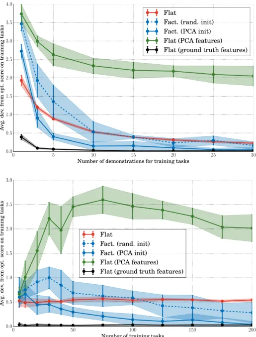
In the results presented here, the demonstrated tasks were generated from a dictionary of 5 primitive reward functions. No feature is used to parametrize rewards: they are represented as deterministic functions from state-action pairs to a real number, which corresponds to a 400 parameters. The expert provides 10 demonstrations for each task, each lasting 10 time steps and 100 tasks are demonstrated.
Results presented in fig. 1 show that the factorial apprentice is capable of using information about the common structure of the various tasks to achieve better performance on each task. The performance of the learner therefore in-creases with the number of demonstrated tasks. When only few demonstrations are given for each task, the demonstrator’s behavior is only observed on a subset of the possible state-action pairs. In such cases, the flat learner often fails to achieve good generalization over all the state space. On the other hand, the factorial learner can benefit from other tasks to complete this information.
We also compare the results with flat learners trained with specific features: the ground truth dictionary (flat, ground truth) and a dictionary learnt by per-forming PCA on the parameters learnt by the flat learners (flat, PCA features).
4.2
Re-use of the dictionary
In order to demonstrate the ability of the factorial algorithm to transfer knowl-edge to new tasks we performed a second experiment. Apprentices are trained similarly to the previous experiment. In the following we call train tasks these tasks. For testing, a new task is generated randomly from the same dictionary of rewards (denoted as test task ) and apprentices observe a single demonstration of the new task. To get meaningful results, this step is reproduced on a number of independent test tasks (typically 100 in the experiment).
Since the task is different from the previous demonstrations, it is not really meaningful for the flat learners to re-use the previous samples or the previously learnt parameters, so the task must be learnt from scratch. On the other hand, the factorial learner re-uses its dictionary as features to learn mixing coefficients for the new task. We also experimented two alternative, simpler, strategies to
3This policy is obtained as a greedy policy on the optimal action value function (with respect to the model of the task, rlearnt), computed by value iteration.
Figure 1: Performance on train tasks The factorial learner overcomes the flat learner by leveraging the features common to all tasks for high number of demonstrated tasks and moderate number of demonstrations for each task. The curves represent the average deviation (lower is better) from the best possible score (the one obtained with perfect knowledge of the task), that is the average of the optimal value function, for different values of the number of demonstrations per training task (top) for a fixed number of training tasks of 100 and for the number of training tasks (bottom), the number of demonstrations for each tasks
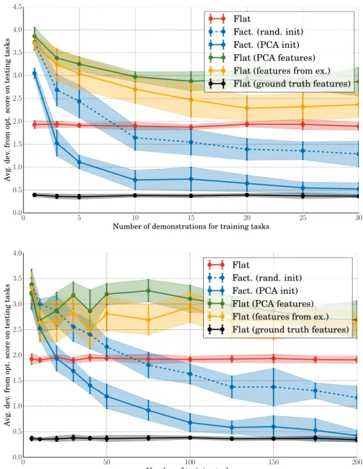
build a dictionary in order to re-use information from the training tasks. The first one consists in using a random selection of rewards learnt during training as features for the new tasks (flat, features from ex.). We use the learnt parameters of 15 training tasks as features. The other one performs a PCA on the rewards learnt during training and uses the five first components as features (flat, PCA features).
Similarly to previous experiment the apprentices are evaluated on their score (according to ground truth reward function) on solving the new task.
Results, presented in fig. 2 are compared for various number of training tasks and demonstration per task. They demonstrate that the factorial learner can re-use its knowledge about the combinatorial structure of the task to learn the new task more quickly. The factorial learner also outperforms the other simple feature construction strategies.
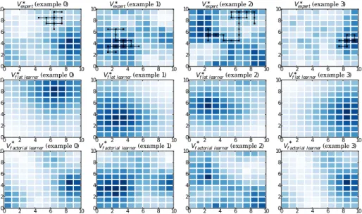
The better ability of the factorial apprentice to generalize over the state space is increased in this setting since only a single demonstration is observed from the expert. Often this demonstration only covers a small part of the state-action space. This phenomenon is illustrated in fig. 3 that represents the true optimal value function together with the expert’s demonstrations, and the learnt value functions by both the flat learner and the factorial one. A typical situation that can be observed in some examples, is that the flat learner’s value function is local to expert’s demonstration, while the factorial learner, that estimates the task in the space of learnt features, can have a good estimate of the value function in parts of the space where no demonstration was provided.
5
Discussion
In this paper we presented a gradient descent algorithm to learn a dictionary of features to represent multiple tasks observed through an expert’s demon-strations with an inverse reinforcement learning approach. The experiments demonstrate that the approach enables the learning of the common structure of the tasks by using transversal information from all the demonstrated tasks. Furthermore it demonstrates and illustrates the fact that this approach enables more accurate representation of new tasks from only one short demonstration, where the classical inverse reinforcement learning approach fails to generalize to unobserved parts of the space due to the lack of adequate features.
The algorithm is compared with naive approaches trying to learn a dictio-nary from task parameters that were inferred through flat inverse reinforcement learning and showed that these approaches fail to learn the relevant structure of the demonstrated tasks. A possible interpretation of this difference is that the PCA approach performs the matrix factorization with respect to the metric of the parameter space, whereas our algorithm uses the more relevant objec-tive cost function. Due to the particular structure of the inverse reinforcement learning problem, namely invariance of the problem with respect to reward
scal-ing, and other transformations [Ng et al.,1999,Neu and Szepesv´ari,2007], the
Figure 2: Performance on test tasks For new task observed through a sin-gle demonstration, the factorial learner outperforms the flat learner by re-using previous knowledge on task features. The curves represent the average devi-ation (lower is better) from the best possible score, for different values of the number of demonstrations per training task (top) for a fixed number of train-ing tasks of 100, and for the number of traintrain-ing tasks (bottom), the number of demonstrations for each tasks being fixed to 10. (Best seen in colors)
0 2 4 6 8 10 0 2 4 6 8 10 V ∗ expert(example 0) 0 2 4 6 8 10 0 2 4 6 8 10 V ∗
f lat learner(example 0)
0 2 4 6 8 10 0 2 4 6 8 10V ∗
f actorial learner(example 0)
0 2 4 6 8 10 0 2 4 6 8 10 V ∗ expert(example 1) 0 2 4 6 8 10 0 2 4 6 8 10 V ∗
f lat learner(example 1)
0 2 4 6 8 10 0 2 4 6 8 10V ∗
f actorial learner(example 1)
0 2 4 6 8 10 0 2 4 6 8 10 V ∗ expert(example 2) 0 2 4 6 8 10 0 2 4 6 8 10 V ∗
f lat learner(example 2)
0 2 4 6 8 10 0 2 4 6 8 10V ∗
f actorial learner(example 2)
0 2 4 6 8 10 0 2 4 6 8 10 V ∗ expert(example 3) 0 2 4 6 8 10 0 2 4 6 8 10 V ∗
f lat learner(example 3)
0 2 4 6 8 10 0 2 4 6 8 10V ∗
f actorial learner(example 3)
Figure 3: The factorial learner achieves a better recognition of new tasks from a single demonstration by using the learnt features. In contrast the flat learner often build a task representation that is local to the demonstration. First row represents the optimal value function (blue is high) for the real task, together with the single demonstration provided by the expert. Second and third row represents the optimal value function for the model of the task as learnt by respectively the flat learner and the factorial learner. Each column corresponds to one of the four first test tasks (from a total of 100). (Best seen in colors)
learning.
An important limitation of inverse reinforcement learning is that it assumes the knowledge of a model of the dynamics of the environment. Therefore it can either be applied to situations where that model is actually known, meaning it is very simple, or where it can be learnt. However the latter brings the new question of the robustness of inverse reinforcement algorithms to errors or gaps in the learnt model. Furthermore, while regular inverse reinforcement learning outputs both a model of the task and a policy that solves it, the factorial ap-proach presented in this section only provides policies for the observed tasks. This means that although a large variety of tasks may be represented by com-bining primitive tasks from the learnt dictionary, it is generally not meaningful to combine the policies in the same way: the agent has to train a policy for these new tasks.
This algorithm can be considered as a first example of feature learning in
the multi-task setup for inverse reinforcement learning. However other
ap-proaches should be explored by further work in order to derive more efficient
algorithms, by for example extending the natural gradient approach fromNeu
and Szepesv´ari[2007] to the dictionary learning setup, or adopting a Bayesian
approach extendingRamachandran and Amir[2007].
Finally constraints can be applied to the learnt dictionary to favor some kinds of solutions. Two examples of such constraints for which many machine learning algorithms have been developed are non-negativity and sparsity. Non-negativity of the coefficients would for example focus on representations that allow primitive behaviors to be added to, but not subtracted from an activity in which they do not appear. Such constraints have been successful in many fields to yield decompositions with good properties, in terms of interpretability but
also sparsity [Paatero and Tapper,1994,Lee and Seung,1999,ten Bosch et al.,
2008,Lef`evre et al.,2011,Hellbach et al.,2009,Mangin and Oudeyer,2013, see for example]. Sparse coding also focuses on a constraint on decompositions to
improve the properties of the learnt elements [Hoyer,2002,Aharon et al.,2005,
Lee et al.,2006]. For example. Jetchev and Toussaint[2011] have shown how enforcing sparsity of a task representation can make this task focus only on a few salient features, thus performing task space inference. Other examples are
given byLi et al.[2010] andHellbach et al.[2009]. Exploring the use of these
constraints together with the techniques presented in this paper constitutes important direction for further work.
References
Pieter Abbeel and Andrew Y Ng. Apprenticeship learning via inverse reinforce-ment learning. In International conference on Machine learning, 2004. Michal Aharon, Michael Elad, and Alfred Bruckstein. K-svd: Design of
dictio-naries for sparse representation. In Proceedings of SPARS, number 5, pages 9–12, 2005.
Javier Almingol, Luis Montesano, and Manuel Lopes. Learning multiple behav-iors from unlabeled demonstrations in a latent controller space. In Interna-tional conference on Machine learning (ICML), 2013.
Monica Babes-Vroman, Vukosi Marivate, Kaushik Subramanian, and Michael Littman. Apprenticeship learning about multiple intentions. In International conference on Machine learning (ICML), number 28, 2011.
Sven Hellbach, Julian P Eggert, Edgar K¨orner, and Horst-michael Gross. Basis
decomposition of motion trajectories using spatio-temporal nmf. In Int. Conf. on Artificial Neural Networks (ICANN), pages 597–606, Limassol, Cyprus, 2009. Springer.
Patrik O Hoyer. Non-negative sparse coding. Technical report, February 2002. Nikolay Jetchev and Marc Toussaint. Task space retrieval using inverse feedback control. In Lise Getoor and Tobias Scheffer, editors, International Conference on Machine Learning, number 28 in ICML ’11, pages 449–456, New York, NY, USA, June 2011. ACM. ISBN 978-1-4503-0619-5.
Daniel D. Lee and H Sebastian Seung. Learning the parts of objects by non-negative matrix factorization. Nature, 401(6755):788–91, October 1999. ISSN 0028-0836. doi: 10.1038/44565.
Honglak Lee, Alexis Battle, Rajat Raina, and Andrew Y. Ng. Efficient sparse coding algorithms. In Advances in Neural Information Processing Systems (NIPS), number 19, 2006.
Augustin Lef`evre, Francis R. Bach, and C´edric F´evotte. Itakura-saito
nonnega-tive matrix factorization with group sparsity. In Acoustics, Speech and Signal Processing (ICASSP), 2011 IEEE International Conference on, number 1, pages 21–24. IEEE, 2011.
Sergey Levine, Zoran Popovic, and Vladlen Koltun. Feature construction for inverse reinforcement learning. Advances in Neural Information Processing Systems, (24):1–9, 2010.
Yi Li, Cornelia Fermuller, Yiannis Aloimonos, and Hui Ji. Learning
shift-invariant sparse representation of actions. In 2010 IEEE Computer Soci-ety Conference on Computer Vision and Pattern Recognition, pages 2630–
2637, San-Francisco, June 2010. IEEE. ISBN 978-1-4244-6984-0. doi:
10.1109/CVPR.2010.5539977.
Olivier Mangin and Pierre-Yves Oudeyer. Learning semantic components from subsymbolic multimodal perception. In the Joint IEEE International Con-ference on Development and Learning and on Epigenetic Robotics (ICDL-EpiRob), number 3, August 2013.
Gergely Neu and Csaba Szepesv´ari. Apprenticeship learning using inverse rein-forcement learning and gradient methods. In Conference on Uncertainty in Artificial Intelligence (UAI), number 23, pages 295–302, Vancouver, Canada, 2007. AUAI Press, Corvallis, Oregon. ISBN 0-9749039-3-00-9749039-3-0. Andrew Y. Ng and Stuart Russell. Algorithms for inverse reinforcement learning.
International Conference on Machine Learning, 2000.
Andrew Y. Ng, Daishi Harada, and Stuart Russell. Policy invariance under re-ward transformations: Theory and application to rere-ward shaping. In Interna-tional Conference on Machine Learning (ICML), number 16, pages 278–287, 1999.
P Paatero and U Tapper. Positive matrix factorization: A non-negative factor model with optimal utilization of error estimates of data values. Environ-metrics, 5(2):111–126, 1994.
Deepak Ramachandran and Eyal Amir. Bayesian inverse reinforcement learn-ing. In International Joint Conference on Artificial Intelligence (IJCAI’07), number 20, pages 2586–2591, 2007.
Nathan D. Ratliff, J. Andrew Bagnell, and Martin A. Zinkevich. Maximum margin planning. In International conference on Machine learning - ICML ’06, number 23, pages 729–736, New York, New York, USA, 2006. ACM Press. ISBN 1595933832. doi: 10.1145/1143844.1143936.
Daniel L. Silver, Qiang Yang, and Lianghao Li. Lifelong machine learning sys-tems : Beyond learning algorithms. In AAAI Spring Symposium Series, pages 49–55, 2013.
Louis F.M. ten Bosch, Hugo Van Hamme, and Lou W.J. Boves. Unsupervised detection of words questioning the relevance of segmentation. In Speech Anal-ysis and Processing for Knowledge Discovery, ITRW ISCA. Bonn, Germany : ISCA, 2008.
Brian D Ziebart, Andrew Maas, J Andrew Bagnell, and Anind K Dey. Maxi-mum entropy inverse reinforcement learning. In AAI Conference on Artificial Intelligence, number 23, pages 1433–1438, 2008.