HAL Id: hal-02071362
https://hal.archives-ouvertes.fr/hal-02071362
Submitted on 18 Mar 2019
HAL is a multi-disciplinary open access
archive for the deposit and dissemination of
sci-entific research documents, whether they are
pub-lished or not. The documents may come from
teaching and research institutions in France or
abroad, or from public or private research centers.
L’archive ouverte pluridisciplinaire HAL, est
destinée au dépôt et à la diffusion de documents
scientifiques de niveau recherche, publiés ou non,
émanant des établissements d’enseignement et de
recherche français ou étrangers, des laboratoires
publics ou privés.
Feasibility Study of Probabilistic Timing Analysis
Methods for SDF Applications on Multi-Core Processors
Ralf Stemmer, Hai-Dang Vu, Maher Fakih, Kim Grüttner, Sébastien Le
Nours, Sébastien Pillement
To cite this version:
Ralf Stemmer, Hai-Dang Vu, Maher Fakih, Kim Grüttner, Sébastien Le Nours, et al.. Feasibility Study
of Probabilistic Timing Analysis Methods for SDF Applications on Multi-Core Processors. [Research
Report] IETR; OFFIS. 2019. �hal-02071362�
Feasibility Study of Probabilistic Timing Analysis
Methods for SDF Applications on Multi-Core
Processors
Ralf Stemmer
∗, Hai-Dang Vu
†, Maher Fakih
‡, Kim Gr¨uttner
‡,
Sebastien Le Nours
†and Sebastien Pillement
†∗ University of Oldenburg, Germany, Email: [email protected]
† University of Nantes, France, Email: {hai-dang.vu, sebastien.le-nours, sebastien.pillement}@univ-nantes.fr ‡OFFIS e.V., Germany, Email: {maher.fakih, kim.gruettner}@offis.de
Abstract—Early validation of software running on multi-core platforms is fundamental to guarantee functional correctness and that real-time constraints are fully met. In the domain of timing analysis of multi-core systems, existing simulation-based approaches and formal mathematical methods are hampered with scalability problems. In this context, probabilistic simulation techniques represent promising solutions to improve scalability of analysis approaches. However, creation of probabilistic SystemC models remains a difficult task and is not well supported for multi-core systems. In this technical report, we present a feasibility study of probabilistic simulation techniques con-sidering different levels of platform complexity. The evaluated probabilistic simulation techniques demonstrate good potential to deliver fast yet accurate estimations for multi-core systems.
I. INTRODUCTION
Because of the growing demand in computational efficiency, more and more embedded systems are designed on multi-core platforms. Multi-multi-core platforms are a combination of computation resources (general-purpose processors, special-ized processors, dedicated hardware accelerators), memory resources (shared memories, cache memories), and commu-nication resources (bus, network on chip). Compared to single processor platforms, the sharing of resources in multi-core platforms leads to complex interactions among components that make validation of software and estimation of extra-functional properties very challenging.
System level design approaches have been proposed to allow performance estimation of hardware/software architec-tures early in the design process. In system level design approaches, workload models are used to capture the influence of application execution on platform resources. Timing prop-erties of architectures and related power consumption can then be assessed under different working scenarios. However, the efficiency of system level design approaches strongly depends on the created HW/SW architecture models that should deliver both reduced analysis time and good accuracy. Especially,
This work has been partially sponsored by the DAAD (PETA-MC project under grant agreement 57445418) with funds from the Federal Ministry of Education and Research (BMBF). This work has also been partially sponsored by CampusFrance (PETA-MC project under grant agreement 42521PK) with funds from the French ministry of Europe and Foreign Affairs (MEAE) and by the French ministry for Higher Education, Research and Innovation (MESRI)
captured workload models should correctly abstract low-level details of system components but still provide good estimates about the whole system performance. High-level component models must capture the possible variability in multi-core platform resources usage caused by cache management, bus interleaving, and memory contention. Creation of efficient architecture models represents thus a time-consuming effort that limits the efficiency of current system level approaches. Because of the growing complexity of architectures, existing real-time analysis methods, i.e., simulation-based and formal mathematical approaches, show limitations to deliver fast yet accurate estimation of timing properties. Novel analysis techniques are thus expected to facilitate the evaluation of multi-core architectures with good accuracy and in reasonable times.
Probabilistic models represent a possible solution to capture variability caused by shared resources on parallel software execution [1]. Quantitative analysis of probabilistic models can then be used to quantify the probability that a given time property is satisfied. Numerical approaches exist that compute the exact measure of the probability at the expense of time-consuming analysis effort. Another approach to evaluate probabilistic models is to simulate the model for many runs and monitor simulations to approximate the probability that time properties are met. This approach, which is also called Statistical Model Checking (SMC), is far less memory and time intensive than probabilistic numerical methods and it has been successfully adopted in different application domains [2]. In the field of embedded system design, executable specifications built with the use of the SystemC language are now widely adopted [3]. SystemC models used for the purpose of timing analysis typically capture workload mod-els of the application mapped on shared computation and communication resources of the considered platform. Timing annotations are commonly expressed as average values or intervals with estimated best case and worst case execution times. The adoption of SMC techniques to analyze SystemC models of multi-core systems is promising because it could deliver a good compromise between accuracy and analysis time, yet it requires a more sophisticated timing model based
on probability density functions, inferred from measurements on a real prototype. Thus, the creation of trustful probabilistic SystemC models is challenging. Since SMC methods have rarely been considered to analyze timing properties of applica-tions mapped on multi-core processors with complex hierarchy of shared resources, exploring their application on trustful probabilistic SystemC models remains a significant research topic.
In this technical report, we present a feasibility study of SMC methods for multi-core systems. The novelty of the established framework is twofold. The first contribution deals with the modeling process, including a measurement-based approach, to appropriately prepare timing annotations and cal-ibrate SystemC models. The second contribution is about the evaluation of SMC methods efficiency with respect to accuracy and analysis time. Evaluation is done by comparing a real multi-core implementation with related estimation results. To restrict the scope of our study, we have considered applications modeled as Synchronous Data Flow Graphs (SDFGs). We have evaluated our framework on a Sobel filter case study. Two configurations of the multi-core processor with different levels of complexity are considered to analyze the relevance and effectiveness of SMC methods.
This technical report is organized as follows. In Section II we provide an overview and discussion of relevant related work. In Section III we provide background information on our chosen SDF model, considered multi-core timing effects and the applied SMC methods. Section IV presents the established modeling and analysis approach. The experimental results are described in Section V. Section VI discuss the benefits and limitations of the presented approach.
II. RELATEDWORK
A. Timing analysis approaches
Timing analysis approaches are commonly classified as (1) simulation-based approaches, which partially test system prop-erties based on a limited set of stimuli, (2) formal approaches, which statically check system properties in an exhaustive way, and (3) hybrid approaches, which combine simulation-based and formal approaches.
Simulation-based approaches: Different simulation-based approaches have been proposed to evaluate multi-core architecture performance early in the design process. In the proposed approaches, models of hardware-software architec-tures are formed by combining an application model and a platform model. In the early design phase, full description of application functionalities is not mandatory and workload models of the application are used. A workload model ex-presses the computation and communication loads (e.g., time, power consumption, memory cost) that an application causes when executed on platform resources. Captured performance models are then generated as executable descriptions and simulated. The execution time of each load primitive is ap-proximated as a delay, which are typically estimated from measurements on real prototypes or analysis of low level simulations. SystemCoDesigner [4], Daedalus [5], SCE [6],
and Koski [7] are good examples of academic approaches; they are compared in [8]. Other existing academic approaches are presented by Kreku et al. in [9] and by Arpinen et al. in [10]. An overview and classification of the considered related work can be found in Table I. Moreover, some industrial frameworks such as Intel CoFluent Studio [11], Timing Architect [12], ChronSIM [13], TraceAnalyzer [14] Space Codesign [15] and Visualsim from Mirabilis Design [16] have emerged also.
Simulation-based approaches require extensive architecture analysis under various possible working scenarios but created architecture models can hardly be exhaustively simulated. Due to insufficient corner case coverage, simulation-based approaches are thus limited to determine guaranteed limits about system properties. One other important issue concerns the accuracy of created models. As architecture components are modeled as abstractions of low level details, there is no guarantee that the created architecture model reflects with good accuracy the whole system performance. Finally, with the rising complexity of many-core platforms, execution of simulation models requires more simulation time.
Formal approaches: Due to insufficient corner case cov-erage, simulation-based approaches are limited to determine guaranteed limits about system properties. Different formal approaches have thus been proposed to analyze multi-core systems and provide hard real-time and performance bounds. These formal approaches are commonly classified as state-based approaches and analytical approaches.
Most of the available static real-time methods are of analyti-cal nature (c.f. [17] for an overview). Since analytianalyti-cal methods depend on solving closed-form equations (characterizing the system temporal behavior), they have the advantage of being scalable to analyze large-scale systems. MPA-RTC [18] and SymTA/S [19] are two representatives of compositional ana-lytical methods for multi-core systems.
Despite their advantages of being scalable, analytical meth-ods abstract from state-based modus operandi of the system under analysis (such as complex state-based arbitration pro-tocols or inter-processor communication task dependencies) which leads to pessimistic over-approximated results com-pared to state-based methods [17]. Many recent approaches for the software timing analysis on many- and multi-core architectures are built on state-based analysis techniques. The two main considered application classes are streaming appli-cations (modeled as synchronous data flow graphs) [20]–[26] and generic real-time task-based applications [27]–[34]. State-based real-time methods are State-based on the fact of representing the System Under Analysis (SUA) as a transition system (states and transitions). Since the real operation states of the architecture behaviour are reflected, tighter results can be ob-tained compared to analytical methods. However, state-based approaches allow exhaustive analysis of system properties at the expense of time-consuming modelling and analysis effort. In [35], the adoption of model-checking for real-time analysis of SDFGs running on multi-processor with shared communication resources is presented. Especially, it is high-lighted in [35] that state-based approaches can hardly address
systems made of high number of heterogeneous components. This approach utilizes timed automata to represent tasks and arbitration protocols for buses and memories. It uses Best-(BCET) and Worst-Case Execution Time (WCET) intervals as lower and upper bounds of the estimated execution time of a specific platform. In our work, we use a timing model based on probability density functions, which allows a more flexible analysis especially in the case of platforms with complex interaction between resources (e.g., cache effect, external shared memory). The approach we investigate uses a combination of probabilistic models and analysis techniques. It is a hybrid analysis approach that can be seen as a trade-off between simulation and state-based verification approaches.
B. Timing analysis approaches based on probabilistic methods Probabilistic models are frequently adopted to model sys-tems where uncertainty and variability need to be considered. In the context of embedded systems, probabilistic models represent a means of capturing system variability coming from system sensitivity to environment and low level effects of hardware platforms. Probabilistic models (e.g., discrete time Markov chains, Markov automata) can be used to ap-propriately capture this variability. Probabilistic models are extensions of labeled transition system and allow variations about execution times and state transitions to be considered. Quantitative analysis of probabilistic models can be used to quantify that a given time property is satisfied. Numerical approaches exist that compute the exact measure of the prob-ability at the expense of time-consuming analysis effort. As an illustration, the adoption of probabilistic model checking for evaluation of dynamic data-flow behaviors is presented in [20]. Markov automata is used as the fundamental probabilistic model to capture and analyze architectures. Characteristics as application buffer occupancy, timing performance, and platform energy consumption are estimated. However, this approach is restricted to fully predictable platforms, with low influence of platform resources on timing variations.
Another approach to analyze probabilistic models is to simulate the model for many runs and monitor simulations to approximate the probability that time properties are met. Statistical Model Checking (SMC) has been proposed as an alternative to numerical approaches to avoid an exhaustive exploration of the state-space model. SMC refers to a series of techniques that are used to explore a sub-part of the state-space and provides an estimation about the probability that a given property is satisfied. SMC designates a set of statistical techniques that present the following advantages:
• As classical model checking approach, SMC is based on a formal semantic of systems that allows to reason on behavioral properties. SMC is used to answer qualitative questions (Is the probability for a model to satisfy a given property greater or equal to a certain threshold?) and quantitative questions (What is the probability for a model to satisfy a given property?).
• It simply requires an executable model of the system that can be simulated and checked against state-based
properties expressed in temporal logics. The observed executions are processed to decide with some confidence whether the system satisfies a given property.
• As a simulation-based approach, it is less memory and time intensive than exhaustive approaches.
Various probabilistic checkers support statistical model-checking, as for example UPPAAL-SMC [36], Prism [37], and Plasma-Lab [38]. This approach has been considered in various application domains [39].
The usage of UPPAAL-SMC to optimize task allocation and scheduling on multi-processor platform is presented in [40]. Application tasks and processing elements are captured in a Network of Price Timed Automata (NPTA). It is considered that each task execution time follows a Gaussian distribution. In the scope of our work, we especially focus on the prepara-tion process of probabilistic models of execuprepara-tion time. Besides, we consider different platform configurations with different levels of predictability to evaluate the accuracy and analysis time of SMC methods.
Authors in [41], [42] propose a measurement-based ap-proach in combination with hardware and/or software ran-domization techniques to conduct a probabilistic worst-case execution time (pWCET) through the application of Extreme Value Theory (EVT). In difference to their approach, we apply a Statistical Model Checking (SMC) based analysis capturing the system modus operandi. This enables the obtainement of tighter values compared to the EVT approach. Yet our method could benefit from their measurement methodology.
An iterative probabilistic approach has been presented by Kumar [43] to model the resource contention together with stochastic task execution times to provide estimates for the throughput of SDF applications on multiprocessor systems. Unlike their approach, we apply an SMC based analysis which enables a probabilistic symbolic simulation and the estimation of probabilistic worst-case timing bounds of the target application with estimated confidence values.
In [44] integration of SMC methods in a system-level ver-ification approach is presented. It corresponds to a stochastic extension of the BIP formalism and associated toolset [45]. An SMC engine is presented to sample and control simulation execution in order to decide if the system model satisfies a given property. The preparation process of time annotations in system model is presented in [1] where a statistical inference process is proposed to capture low-level platform effects on application execution. A many-core platform running an image recognition application is considered and stochastic extension of BIP is then used to evaluate the application execution time. A solution is presented in [46] to apply SMC analysis methods for systems modeled in SystemC. The execution traces of the analyzed model are monitored and a statistical model checker is used to verify temporal properties. The monitor is automatically generated based on a given set of variables to be observed. The statistical model-checker is implemented as a plugin of the Plasma-Lab. In the scope of our work, we adopt the approach presented in [46] to analyze time properties of multi-core systems modeled with SystemC.
The adoption of SMC methods to timing analysis of multi-core systems is promising because it could deliver good compromise between accuracy and analysis time. However, creation of trustful probabilistic models remains a difficult task and is not well supported for multi-core systems. Especially, to the best of our knowledge, no work attempted to systematically evaluate the benefits of using SMC to analyze the timing properties of applications based on Synchronous Data Flow (SDF) model of computation on multi-cores, targeting more tightness of estimated bounds and faster analysis times.
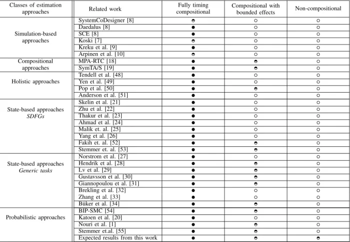
C. Summary of existing analysis approaches
In [47], the authors gave a classification of multi-core architectures w.r.t predictability considerations in their design:
• Fully timing compositional: architectures do not exhibit any timing anomalies1 and the usable hardware platform is constraint to be fully compositional. In this case a local worst-case path can be analyzed safely without considering other paths,
• Compositional with bounded effects:architectures exhibit timing anomalies but no domino effects2,
• Non-compositional: architectures which exhibit both
domino effects and timing anomalies. The complexity of timing analysis of such architectures is very high since all paths must be examined due to the fact that a local effect may influence the future execution arbitrarily. The main discussed approaches are classified in Table I according to the above identified three categories of platforms. We have estimated the efficiency of the approaches for each kind of platforms (well supported , partially supported , not well supported ).
Table I also indicates the position of expected results of our targeted approach. The approach should demonstrate the efficiency of probabilistic methods to analyse multi-core systems. Especially, a significant achievement would be the analysis of non-compositional architectures.
All of the above mentioned analysis approaches rely on the estimation of execution times. For the simulation-based and some probabilistic approaches, the estimation can be per-formed through a detailed simulation model at instruction- or even cycle-accurate level. This involves very time consuming simulations and belongs to the class of measurement-based execution time analysis techniques, that have to deal with the rare-event problem3. Another technique is timing
back-annotation to functional or analytical system models, applying timing measurement or static timing analysis approaches. For most real-time systems, the Worst-Case Execution Time (WCET), which is a safe upper bound of all observable execution times, is the most relevant metric. Sometimes also
1Timing anomaly is referred to “the situation where a local worst-case
doesn’t contribute to the global worst-case” in [47] e.g. shorter execution time of an actor can lead to a larger response time of the application.
2Domino effectoccurs when the execution time difference is arbitrary high
(cannot be bounded to a constant) between two states (s, t) of the same program (starting in s, t respectively) on the same hardware [47].
3Rare events are events that occur with low frequency but which have
potentially widespread impact, e.g. on the execution time.
Probabilistic Model-Checker SystemC Model ActorA(); sc_core::wait(GetDelay(A)); ActorB(); sc_core::wait(GetDelay(B));
B
A
TileRandom value from file Measurement
φ = G≤T (((delay(A) ≤ d1 ) & (delay(B) ≤ d2 )) (t⇒latency ≤ d))
Stored samples Traces 1 1 1 1 Plasma Lab Real System
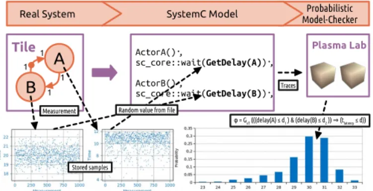
Fig. 1: Example of applying statistical model checking on a two-actor SDF application executed on a single tile. The measured timing characteristic used in a SystemC model can be seen in the left plots. These measured execution time samples were randomly selected by the GetDelay function. The blue histogram is the result of the end-to-end latency analysis with Plasma Lab.
the Best-Case Execution Time (BCET) is considered in combi-nation with WCET in a [BCET, WCET] interval. Static timing analysis [56] is the state-of-the-art technique to determine the WCET and BCET respectively. With the adoption of todays multi-core systems, limitations of static timing analysis are becoming apparent [47].
For modern multi-core architectures, measurement-based approaches can overcome many problems of static timing analysis. But this comes at a price, since measurement-based timing analysis is facing the rare-event problem, its analysis results are either largely over-approximated (using a large safety margin) or untrustworthy (due to a missing probability analysis). To overcome these challenges for measurement-based timing analysis for modern processors and multi-core systems, the work in the context of the projects PROARTIS4
[57] and PROXIMA5 [58] propose a new way for timing
analysis. Instead of applying improved static analysis, a mea-surement based approach in combination with hardware and/or software randomization techniques to conduct a probabilistic worst-case execution time (pWCET) through the application of extreme value theory (EVT) has been proposed. Both projects have successfully assessed that measurement based execution time analysis with the combination of EVT can be used to construct a worst-case probability distribution. In difference to these approaches, we apply an SMC-based analysis approach to consider a full system modus operandi. Furthermore, we are applying the analysis on a set of restricted and well analyzable Models of Computation (MoCs)
The established approach combining probabilistic execution times and probabilistic analysis methods is presented in the next section.
Classes of estimation
approaches Related work
Fully timing compositional
Compositional with
bounded effects Non-compositional
Simulation-based approaches SystemCoDesigner [8] Daedalus [8] SCE [8] Koski [7] Kreku et al. [9] Arpinen et al. [10] Compositional approaches MPA-RTC [18] SymTA/S [19] Holistic approaches Tendell et al. [48] Yen et al. [49] Pop et al. [50] Anderson et al. [51] State-based approaches SDFGs Skelin et al. [21] Zhu et al. [22] Thakur et al. [23] Ahmad et al. [24] Malik et. al. [25] Yang et al. [26] Fakih et. al. [52] Stemmer et. al. [53] State-based approaches Generic tasks Norstrom et al. [27] Hendrik et al. [28] Lv et al. [29] Gustavsson et al. [30] Giannopoulou et al. [31] Brekling et al. [32] Zhang et al. [33] B¨uker et al. [34] Probabilistic approaches BIP-SMC [54] Katoen et al. [20] Nouri et al. [1] Stemmer et.al. [55]
Expected results from this work
TABLE I: Classification of related work and main references.
III. PRELIMINARIES
A. SDFGs
A synchronous data-flow graph (SDFG) [59] is a directed graph (see example in Fig.1, Sobel filter in Fig.3a) which consists mainly of nodes (called actors) modeling atomic functions/computations and arcs modeling the data flow (called channels). SDFGs consume/produce a static number of data samples (tokens) each time an actor executes (fires). An actor can only be executed, when there are enough tokens available on its ingoing channels.
Definition 1: (SDFG) A synchronous dataflow graph is defined as SDF G = (A, C), which consist of a finite set A of actors A and a finite set C of channels C.
1) a finite set A of actors A.
2) a finite set C of channels C. A channel is a tuple C = (Ri, Ro, B) with
a) The input rate Ri defining the number of tokens that
can be written into the channel during the write phase of an actor.
4Probabilistically Analysable Real-Time Systems (http://www.
proartis-project.eu)
5Probabilistic real-time control of mixed-criticality multicore and manycore
systems (http://www.proxima-project.eu)
b) The output rate Rodefining the number of tokens that
will be read from the channel during the read phase of an actor.
c) The buffer size B in number of tokens.
In the context of SDFGs, an iteration of an SDFG (refer to [35] for more formal definitions) is completed when the initial tokens’ distribution on all its channels is restored. The end-to-end latencyis the time starting from activating the first instance of the source actor, executing the SDFG application till the last instance of the sink actor is finished.
B. Multi-Core Timing Effects
Variations of the execution time can be caused by two main sources:
1) Software induced: Data dependencies in the algorithm, leading to different execution paths of the software (dif-ferent branches or number of loop iterations, which are taken).
2) Hardware induced: Depending on the processor and memory architecture, different timing variations can oc-cur, these can be further grouped into
a) local effects: only dependent on the properties and the state of the processor architecture where the software is executed on. This includes data dependent execu-tion times of instrucexecu-tions, branch predicexecu-tion, and local cache misses.
b) global effects: dependent on the usage and properties of shared resources used by multiple processors. This includes access to a shared bus, shared memory and shared caches (2nd level cache).
The software induced timing effects can be handled though appropriate algorithm design (i.e. by avoiding data dependent loops) and a static path analysis. Hardware induced local effects can be handled (if known and well documented) by static Worst-Case Execution Time (WCET) analysis. For the global effects, static analysis is extremely difficult or even impossible for specific multi-core platforms. For this reason, measurement based timing analysis approaches are currently being employed to cope with these difficult timing interfer-ences. In this paper we are considering timing effects of all of the described classes.
C. Statistical Model-Checking Methods
Consider a probabilistic system S and a property ϕ. Statis-tical Model Checking (SMC) refers to a series of simulation-based techniques that can be used to answer two types of question [60]: (i) What is the probability that S satisfies ϕ (quantitative analysis), written P r(S |= ϕ)? And (ii) Is the probability that S satisfies ϕ greater or equal to a threshold θ (qualitative analysis), written P r≥θ(S |= ϕ) ? The core idea
of SMC is to monitor a finite set of simulation traces which are randomly generated by executing the probabilistic system S. Then, statistical algorithms can be used to estimate the probability that the system satisfies a property. In the scope of this paper, we consider two algorithms: Monte Carlo with Chernoff-Hoeffding bound to answer the quantitative question and Sequential Probability Ratio Test (SPRT) for qualitative question. Although SMC only provides an estimation, the algorithms presented below offer strict guarantees on the precision and the confidence of the test.
Let p = P r(S |= ϕ) be the probability that the system satisfies a certain property ϕ. The methods which can quantify p are based on the techniques of Monte Carlo with Chernoff-Hoeffding bound [61]–[63]. Given a precision δ, an estimation procedure consists on computing an approximation p0 such that |p0− p| ≤ δ with confidence α, i.e., P r(|p0− p| ≤ δ) ≥ 1 − α. Given B1, ..., Bn as n discrete random variables with
a Bernoulli distribution of p associated with n simulations of the system. We denote bi as the outcome of each Bi, which
is 1 if the simulation satisfies ϕ and 0 otherwise. Based on Chernoff-Hoeffding bound [64], p0 can be approximated as p0 = (Pn
i=1bi)/n and the minimum number of observations
that guarantees P r(|p0− p| ≤ δ) ≥ 1 − α can be computed as n ≥ δ42log(
2 α).
The statistical methods to answer the qualitative question are based on hypothesis testing (see details in [46], [1]). The principle of these methods is to determine whether the probability that the system satisfies a property is greater than a given bound: p ≥ θ? In [65], Younes proposed SPRT as an hypothesis testing algorithm, in which the hypothesis H0:
p ≥ p0 = θ + δ is tested against the alternative hypothesis
H1: p ≤ p1= θ − δ. The strength of a test is determined by
two parameters (α, β) which are the probability of accepting H0 when H1 holds (type I error or false negative), and the
probability of accepting H1 when H0 holds (type II error
or false positive). The interval [p0, p1] is referred to the
indifference regionof the test which contains θ.
Analysis results using these two statistical algorithms will be presented in Section V.
D. Statistical Timing Properties
In this paper, we consider the properties specified in Bounded Linear Temporal Logic (BLTL). This logic enhances Linear Temporal Logic (LTL) operators with time bounds. A BLTL formula ϕ is defined over a set of atomic propositions AP , the logical operators (e.g., true, f alse, ¬, → and ∧) and the temporal modal operators (e.g., U , X, F , G, M and W ) by the grammar as follows.
ϕ := true | f alse | ap ∈ AP | ¬ ϕ | ϕ1 ∧ ϕ2 | ϕ1 U≤T ϕ2
The time bounds T is the duration of one simulation run during which we analyze the property. Temporal modality F , for ”eventually”, can be derived from the ”until” U as F≤T ϕ = true U≤T ϕ. It means that the property ϕ is
eventually satisfied within T . Similarly, temporal modality G for ”always” can be derived from F as G≤T ϕ = ¬F≤T
¬ϕ. This equation can be explained as: the hypothesis that the property ϕ is not satisfied within T will not occur or the property ϕ is always satisfied within T . The semantic of BLTL logic is the semantic of LTL logic restricted to a time interval (see details in [46]). Consider the example in Fig. 1, the computation times of two actors A and B stay below threshold values d1, d2: delay(A) ≤ d1 and delay(B) ≤ d2.
The BLTL formula to express the probability that the end-to-end latency t latency always stays below a threshold value d within T is ϕ = G≤T(((delay(A) ≤ d1)&(delay(B) ≤
d2)) => (t latency ≤ d)).
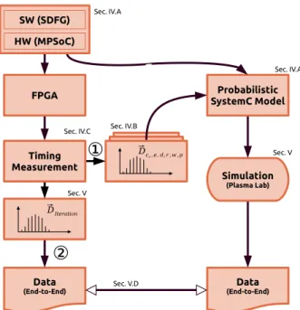
IV. APPROACH
Our approach is shown in Fig. 2. We start with a model of our implemented system. This model consists of an SDF computation model of an application that is mapped and scheduled on a multi-processor hardware platform with shared memory communication. The system model is described in section IV-A in detail. The hardware architecture gets instan-tiated on an FPGA and the modeled application is executed on this system. We then measure the timing behavior of the application running on this system for our model (see arrow
1
in Fig. 2). The results of the end-to-end latency analysis of our model is then compared to the actual measured end-to-end latency (see arrow in Fig. 2) in section V-B.2
A. System Model
In this section, we explain our software and hardware model, as well as the mapping and scheduling of the software on the hardware. Furthermore, we describe how we model the timing behavior of the system.
Data (End-to-End) Data (End-to-End) Simulation (Plasma Lab) Probabilistic SystemC Model FPGA SW (SDFG) HW (MPSoC) Sec. IV.A Sec. IV.C Sec. V Sec. IV.A
②
①
Sec. V.D Sec. V Timing Measurement Sec. IV.B ⃗Dc x,e , d,r ,w ,p ⃗DIterationFig. 2: Overview of our approach to use measured execution time for a simulation-based stochastic end-to-end latency analysis. The annotation refers to the paper section describing the individual steps.
Tile 0 Tile 1 BUS 0 (Data) Shared Memory Get Pixel GY GX ABS 81 81 81 81 1 1 1 1 (a) (b) Get Pixel ABS GX GY Cache 1 Cache 0 DDRShared Memory BRAM
BUS 1 (Instructions + Data)
Private Memory Private Memory
Actors FIFOs Cache Setup DDR Ⓒ BRAM Ⓑ yes 2 BRAM Ⓐ BRAM Ⓑ no 1 Ⓐ Ⓑ Ⓒ Ⓐ
Fig. 3: a) A Sobel filter modeled as an SDFG. A 9×9 pixels segment of an image is read by GetPixel actor and is sent to the GX and GY actors. The result of the convolutions in GX and GY is sent to the
ABSactor where a pixel for the resulting image is calculated.
b) Our platform consisting out of two tiles with caches and two shared memories. The Sobel filter’s actors are mapped to the tiles. The instructions and local data of the actors use either the private
memory or the shared DDRA . The channels for data exchangeC
between the actors are mapped to the shared BRAM . Due toB
the added caches and the DDR memory, the timing behavior of the system becomes highly non-deterministic.
1) Model of Computation: The SDF model: The Sobel filter (see Fig. 3a), used in our experiments, follows SDF semantics that are described in subsection III-A.
SDF model of computation offers a strict separation of computation and communication phases of actors. During the computation phase, no interference with any other actor can
occur, if the respective code is mapped to dedicated memories (see setup 1 in Fig. 3b). We later weaken this constraint and run the code from a shared DDR memory (see setup 2 in Fig. 3b). This obviously leads to interferences and extra delays between the actors accessing shared memories which will be also taken into consideration by our probabilistic model.
The channels are implemented as FIFO buffers on a shared memory.
The actors are static scheduled and will not be preempted. Iterations can overlap over time. In our example GetPixel of one iteration will be executed at the same time ABS gets executed from the iteration before (See Fig. 4.
2) Model of Architecture: The hardware model: We started with a hardware model of a composable system that uses multiple independent tiles to execute applications as determin-istic as possible. Interference occurs only when applications explicitly access shared resources like shared memories or a shared interconnect. We then extend this hardware with a common memory for the instructions of the software executed on the tiles (Fig. 3b).
Definition 2: (Tile)A tile is a tuple T = (P E, Mp) where
P E is the processing element and Mp is the private memory
only accessible by the processing element. A tile can execute software without interfering with other tiles as long as the software only accesses the private memory.
Definition 3: (Execution Platform) An execution platform is defined as EP = (T , Ms, Ca, I) consisting of a finite set
T of tiles T as defined in Def. 2, a finite set Ms of shared
memory Ms, a finite set Cs of dedicated caches Ca for each
tile, and a finite set I of shared interconnects I. While a tile can be connected to multiple interconnects, we assume that every memory is connected to only one interconnect. Furthermore we assume that tiles can only communicate via a shared memory.
In the experiments, without loss of generality, the used inter-connects support a first-come first-serve-based communication protocol. The EP1and EP2for the two setups in Fig. 3b) can
be expressed as follows:
EP1= ({tile0, tile1}, {BRAM }, {}, {BU S0}) (1)
EP2= ({tile0, tile1}, {DDR, BRAM }, {Cache0, Cache1}, {BU S0, BU S1})
(2)
As shown in Fig. 3b, in the first setup (EP1) the platform
consists of two tiles with local data and instruction memories connected with a data bus to a shared memory, through which inter-tile communication takes place. This setup is full composable such that the computation phases of any actor (taking place locally on private memory) can be considered independent from communication phases (taking place via the data bus supporting a single-beat transfer style). For the second setup (EP2) the computation code of actors is placed on a
DDR memory where, with the help of a cache controller (one for each tile), the code is accessed via a data/instruction bus (see BUS1 in Fig. 3b). Also here the inter-tile communication takes place via the data bus (BUS0) and the shared BRAM memory.
ABS r GetPixel GX GY ABS r r r w r Iteration i MB0 MB1 di , end-to-end w GetPixel GY w r w w di ,cGetPixel di ,cABS di ,cGX di ,cGY di+1, cGetPixel
(
di ,WTGetPixel →GX+di ,WTGetPixel →GY)
di , RTGetPixel → GY di ,WTGY→ ABS
di−1, cGY
di−1, cABS
(
di ,RTGX →ABS+di , RTGY → ABS)
di , RTGetPixel → GXw w
r
di ,WTGX →ABS
Fig. 4: Expected actor and phase activation for one iteration i (orange - start of the first actor to the end of the last actor) The annotated
delays di,x ∈ ~D are our measured values for iteration i. di,RT
represent the read-time (equ. 4) and di,W T the write-time (equ. 3) of
the communication. di,cx is the computation time an actor x needs
in iteration i. The End-To-End latency di,end-to-endis the delay of one
iteration (cp. [55])
B. Timing Model
All timings are related to the mapped software (i.e. SDF actors and channels) on a specific hardware. For this reason, the annotation of any delays (in cycles) to the models takes place after the mapping and scheduling process, as shown in Fig. 4. While the execution of an actor’s computation phase on a specific tile can be represented by a single delay d ∈ ~Dc
(see Def. 4) for each considered execution, the communication timing model requires more effort.
To follow the SDF semantics, communication is real-ized using a FIFO buffer. Communication between actors is modeled considering every single memory access, including synchronizing meta data, plus some time consumed by the computational parts of the FIFO implementation. For our implementation of the FIFO buffer the time for writing t tokens is described by:
dW riteT okens(t) = (n + 2) dr+ (t + 1) dw+ n · dp+ de (3)
The time for reading t tokens to the FIFO is:
dReadT okens(t) = (n + t + 2) dr+ 2 · dw+ n · dp+ dd (4)
The read and write phase of an actor expects a ready (filled or empty) FIFO buffer for each channel connected to the actor. During these phases the state of the buffer is checked via polling. Each polling iteration takes a time of dp that is
defined by the developer but can vary when executed from shared memory or due to caching effects. The amount n of polling iterations is determined during the analysis of the model and varies between each SDF execution iteration i. Accessing memory consumes read time dr∈ ~Dror write time
dw ∈ ~Dw for each token t that is transferred as well as for
updating meta data. Furthermore, it takes some computation time for managing the FIFO. These delays are the enqueue delay de ∈ ~De of the write phase or the dequeue delay
dd ∈ ~Dd for the read phase. Delays can vary in each SDF
execution iteration i.
Definition 4: (Time Model) D is defined as a set of delay vectors ~D ∈ D with probable execution delays, consisting of the following delay vectors:
• D~c∈ D: The computation time of an actor A ∈ A.
bus tile 0 Execute() b_transport() shared memory b_transport() tile 1 Execute()
Fig. 5: Setup of our Simulation with SystemC TLM. Two tiles are connected to a shared memory via interconnect. The interconnection
to the shared DDR memory (as given in EP2, see Setup 2 in
Fig. 3b) for the instructions and local data is not explicitly modeled in SystemC. They are implicit in the timing data annotated to the model.
• D~e, ~Dd∈ D: The enqueue and dequeue time that
repre-sents the computation time of the FIFO driver.
• D~r, ~Dw ∈ D: The time to read and write to a memory
M ∈ Mp ∪ Ms. For shared memories this delay
also includes the overhead of the interconnect I ∈ I communication.
• D~p: A polling delay when an actor Ax∈ A tries to access
a FIFO that is blocked (not enough tokens, or not enough free buffer space).
For all above delays, when the corresponding software components need to be loaded from shared memories via caches (like the case in setup 2, see Fig. 3b), the interference with other actors and caching effects is also captured in the corresponding delay vectors. It is assumed that for different mappings the influences of the cache on the execution time of an actor is similar.
C. Probabilistic SystemC Model
The SystemC model is a representation of the whole system. It models the mapped and scheduled SDF application on a specific hardware platform. As shown in Fig. 5 it consists of three major parts: 1) the tile modules for simulating the actors’ execution on a tile, 2) the bus module that simulates the bus behavior (arbitration and transfer) and 3) the shared memory module for the read and write access to the shared memory on which the SDF channels are mapped. For this paper, as seen in Fig. 5, we didn’t explicitly model the caches, the DDR memory and its bus (BUS1), as given in EP2 (Setup 2 in
Fig. 3b). Instead, for simplification reasons, we capture the timing influence of those components (latency times of the cache, bus transfer and memory latency for loading and storing instructions) in the measured actors’ execution times being executed from this memory. It remains interesting for future research to see how the explicit modeling of these elements in the SystemC model would improve the accuracy of EP2
analysis results.
The behavior of the SDF application is simulated as an SC THREADof the tile module. This module also implements the read and write phases of the actors that run on those tiles. The computation phase of an actor is a simple wait statement using the actors’ computation time ~Dc.
The read and write phase are modeled in more details. They are methods that implement a FIFO behavior that follows the
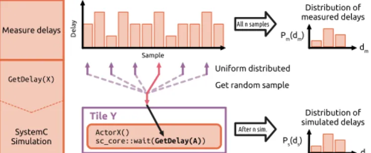
Measure delays After n sim. Distribution of measured delays Distribution of simulated delays Pm(dm) dm Ps(ds) ds Tile Y ActorX() sc_core::wait(GetDelay(A)) All n samples Uniform distributed GetDelay(X) D el ay Sample
Get random sample SystemC
Simulation
Fig. 6: Process of annotating the SystemC model with measured delays from the real system shown for an example actor ActorX on a tile Y. The measured delays are stored in a file (top). The SystemC model (bottom) then gets a random value (center) from that file as delay for the simulation. So the distribution of delays for the simulation are similar to the distribution of the measured delays.
SDF semantics. Both, read and write phases are divided into multiple sections. Each section has a different delay annotation
~
De, ~Dd and ~Dp as described in IV-B.
The bus module manages the arbitration using First Come First Server (FCFS) strategy. The shared memory simply distinguishes read ( ~Dr) and write ( ~Dw) access. Depending on
the access type, it proceeds the simulation time by the related time.
In the SystemC model, the probabilistic timing information can be modeled with the distributions provided by GNU Scientific Library (GSL) [66]. In the case of the Sobel Filter, we consider the computation time of four actors GetPixel, GX, GY, ABS and the communication time to read/write data on the channels or on shared memory. In each iteration of the SystemC model, a computation time or communication time is assigned to a value that is either randomly chosen from the a) uniform, b) normal distributions of the measured delays or c) from a text file containing the raw measured delays of software components (we refer to as injected data). Any other distribution can be used.
To apply the uniform distribution, we choose a random value in the interval of [BCET, WCET]. While in the normal distribution, we consider the mean µ and the variance σ of the corresponding measured delays.
To improve the accuracy of the uniform/normal distributions it is desired to model a probability distribution that accurately reflects the distribution of the measured delays. This is realised by reading a random value (see GetDelay(A) in Fig. 6) for every component (e.g. an actor delay) from a text file that provides all measured delays of this component (we refer to as injected data). This process from measuring an actor to simulating its timing behavior is shown in Fig. 6. The same process is applied for modeling the communication. The measured delay of a random iteration of the actual executed actor gets collected in a file containing all samples of the execution times of that specific actor. So after measurement, there exists files of delays for each delay vector described Def. 4 in Sect. IV-B. To use these data inside the simulation, a function GetDelay (Fig. 6) selects a random value from
the measured raw data file. The distribution of the randomly selected delays is uniform. This achieves a similar delay distribution of the simulated actor compared to the real actor as we will show in the experiments section.
D. Statistical Model-Checking of SystemC Models
The statistical model-checker workflow that we consider takes as inputs a probabilistic model written in SystemC language, a set of observed variables, a BLTL property, and a series of confidence parameters needed by the statistical algorithms, as shown in Fig. 7. First, a monitor model is generated by the Monitor and aspect-advice generator (MAG) tool proposed by V.C Ngo in [46]. Then, the generated monitor and the probabilistic system are instrumented and compiled together to build an executable model. In the simulation phase, Plasma Lab iteratively triggers the executable model to run simulations. The generated monitor observes and delivers the execution traces to Plasma Lab. An execution trace contains the observed variables and their simulation instances. The length of traces depends on the satisfaction of the formula to be verified. This length is finite because the temporal operators in the formulas are bounded. Similarly, the required number of execution traces depends on the statistical algorithms in use supported by Plasma Lab (e.g., Monte Carlo with Chernoff-Hoeffding bounds or SPRT).
The executable model is built with three main steps, as illus-trated in Fig. 8: Generation, Instrumentation and Compilation. Users create a configuration file that especially contains the properties to be verified, the observed variables and the tempo-ral resolution. The configuration file is then used by the MAG tool to generate an aspect-advice file and a monitor model. The aspect-advice file declares the monitor as a friend class of the SystemC model, so that the monitor can access to the private variables of the observed model. The monitor model contains a monitor class and a class called local observer. The local observer class contains a callback function that invokes step() function of the appropriate monitor class at a given sampling point during the simulation [67]. The step() function captures the value of the observed variables and their instances to produce execution trace. The temporal resolution specifies when the set of observed variables is evaluated by the monitor during the simulation of the SystemC model. In the Instrumentation step, the SystemC model and the generated monitor are instrumented by AspectC++ with the help of the aspect-advice file. The instrumented models are linked to the libraries of SystemC and compiled by g++ compiler in the Compilation step to build an executable model. Afterward, users run the Plasma Lab to verify the property.
V. EXPERIMENTS
In this section we describe our experiments and discuss the results.
A. Experiment Definition
In our experiments we use two different configurations of our system. Our platform is shown in Fig. 3b and consists
SystemC Probabilistic Model Observed Variables Property In BLTL Parameters α, β, Ɛ, δ Generation Instrumentation Compilation Observed Model Monitor Executable Model Plasma Lab Monte Carlo/SPRT Result
Input Output Executable
Model Process Traces
Triggers
Fig. 7: Generation and instrumentation of SystemC models and interaction with Plasma Lab statistical model checker.
of two MicroBlaze processors as processing elements. First the private memories of the tiles were used for local dataA
(e.g. stack and heap) and instructions of the actors mapped on that tile. Then the private memory gets replaced by a shared memory .C
The memory for the local data and instructions are con-nected to a different interconnect than the shared memory for inter-processor communication. For the communication between the actors, the channels are mapped onto a shared BRAM Memory (Fig. 3b ).B
In our first experiment, we execute the actors from a private BRAM memory (Fig. 3b ) that is exclusively connected toA
each tile. So there is guaranteed that loading instructions and accessing private data (e.g. from the stack) is deterministic and does not interfere with the other tile.
In the second experiment, we use the shared DDR memory instead of the private memory. (Fig. 3b ) The DDR memoryC
is connected via a second bus to the tiles and does not interfere with the bus used to access the SDF channels’ FIFO buffers. In this setup, the two tiles are no longer independent from each other. This will lead to a higher variance in the execution time distribution.
The interconnect for inter-tile communication uses First Come First Serve arbitration and a single beat transfer pro-tocol. The caches that are used in the second setup use burst transfer to synchronize with the DDR Memory .C
The four actors, GetPixel, GX, GY and ABS, of the applica-tion (Fig. 3b) are mapped onto the tiles as shown in Fig. 3b. Instructions and local data like the heap and the stack are mapped to private memory or to a shared DDR memoryA
C
.
In addition, channels used for communication between actors are mapped to the shared Block RAM memory .B
These channels are organized as FIFO buffers with 4 Bytes for each token and the buffer size is fixed to the input rate of each actor. The mapping and scheduling is fixed for all
experiments.
The measurement technique, we use in the experiments, to get the different delays vectors of different components is based on one presented in [68]. An IP-Core which is con-nected via a dedicated AXI-Stream bus to communicate with each MicroBlaze processor without interfering with the main system buses, is used. The measured cycle-accurate timings were forwarded via an UART interface without influencing the timing behavior of the platform under observation. In order to achieve that, the code of the application is instrumented in a minimal way (for details refer to [68]).
The multicore system is instantiated on a Xilinx Zynq 7020 with external DDR3-1333 memory.
B. End-to-end Timing Validation
In this subsection, we evaluate the best-case and worst-case end-to-end latencies, denoted in the following as BC latency and WC latency. We declare the end-to-end latency as an observed variable t latency in the configuration file used for the SystemC model generation. To quantitatively evaluate the end-to-end latency, the analyzed property is: ”What is the probability that the end-to-end latency stays within an interval [d1,d2]?”. This property can be expressed in BLTL with the
operators ”eventually” as shown in formula 5.
ϕ = F≤T((t latency ≥ d1)&(t latency < d2)) (5)
This property is then analyzed through a finite set of simu-lations controlled by Plasma Lab. In each simulation, Plasma Lab observes the end-to-end latency of a particular iteration to determine the probability that the end-to-end latency stays in the interval [d1, d2]. Fig. 9a and Fig. 9b present the probability
evolution over the intervals [d1, d2] for the two experiments
presented in Section V-A. In both experiments, we compare the real measured end-to-end latency data with the analysis results. We use the Monte Carlo algorithm with Chernoff-Hoeffding bound with absolute error δ = 0.02 and confidence 1 − α = 0.98. It means that the analysis results guarantee the following condition: P r(|p0− p| ≤ 0.02) ≥ 0.98 (see Section III.C for details).
In the first experiment, the computation time of the actors is modeled by using the uniform and normal distributions. We consider also the injected computation time data. Based on the measured results, the communication time varies in a small interval. Since the measured communication time varies within limited number of values, it is reasonable to apply the uniform distribution to model the variation of the communication time. Fig. 9a presents the probability evolution over the intervals [d1, d2] for the first experiment. The end-to-end latencies
obtained from the SystemC model are close to the measured end-to-end latency with a similar range of variation for the different distributions. In the two cases, the WC latencies are over-estimated. We also analyze the SystemC model by applying the injected data which represent the measured data for both computation and communication time. The achieved
Configuration file Aspect-Advice file Monitor MAG Generation SystemC Model AspectC++ Instrumented Model Instrumentation g++ Executable Model Compilation Patched SystemC
Fig. 8: Successive generation, instrumentation and compilation steps to build SystemC executable model.
TABLE II: Comparison of the end-to-end latencies of the analysis with the different distributions compared with the measured data. While for setup I a normal distribution is sufficient, in setup II the observed worst-case was only covered with the actual distribution of the delays.
Subject BC latency I WC latency I BC latency II WC latency II
Measured data 38170 38806 290004 293970
Uniform/Uniform [39300, 39400] [40000, 40100] [277000, 278000] [292000, 293000] Normal/Uniform [39400, 39500] [39900, 40000] [277000, 278000] [291000, 292000] Injected data [39400, 39500] [39900, 40000] [319000, 320000] [327000, 328000]
results do not significantly variate between the uniform, nor-mal distributions and the injected data.
In the second experiment, we follow the same analysis pro-cess, as presented in the first experiment. In Fig. 9b, the uni-form and normal distributions clearly under-estimate the WC latency. Moreover, the interval of variation is larger than the interval of the measured latency. However, the achieved end-to-end latency of the injected data clearly over-approximates the measured WC latency since the chosen delay values are based on the exact measured delay values. The interval of variation is also closer to the interval of the measured latency. This can be explained that the caches in this experiment cause a large variation in communication time. The applied uniform distribution shows a poor representation of the variation of the communication time in such a complex architecture.
The bias between the real-measured latency and the sim-ulated latencies comes from a pessimistic communication model and the lack of consideration of data dependencies between actors. In the real application, the two actors GX and GY have equal execution time in one iteration due to there symmetry. The ABS actor waits for the slowest dependent actor (GX, GY). In our simulation the execution times of GX and GY gets selected randomly and independently. So that the measured timings for faster executions get covered by the slower execution times.
Tab. II summarizes the BC latency and WC latency obtained from the analysis with the uniform, normal distribution and the injected data compared with the measured data in the two experiments. Given an interval, it takes from 10 minutes to 40 minutes to analyze the property. Further analysis to identify precisely the worst-case end-to-end latency is presented in the next section.
C. Evaluation of Statistical Model Checking Methods We want now to bound the end-to-end latency within a threshold value d for the two experiments. Thus, we analyze the property: ”The cumulative probability that the end-to-end latency (t latency) stays below time bound d”. This property can be translated in BLTL with the operator ”always” as follows (Formula 6).
ϕ = G≤T(t latency ≤ d) (6)
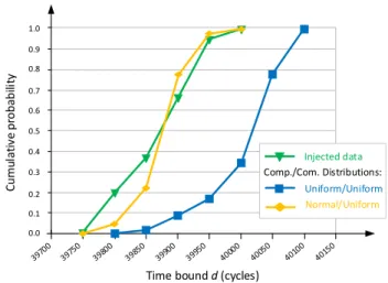
The temporal modal operator G is applied that allows us to check whether all the end-to-end latencies of several successive iterations during the simulation time T stay below d. Therefore, the worst-case end-to-end latency obtained from this property is much more accurate than in the first property. Fig. 10 presents the cumulative probability of the end-to-end latency over time bound d for the first experiment. We compare the analyzed results using the uniform distribution, normal distribution and the injected computation time data. The cumulative probability converges to 1 which means that all the end-to-end latencies analyzed stay below the value d. We can consequently bound the WC latency of the normal distribution and injected computation time under 40 000 cycles (3.08 % higher than the measured WC latency). The bound of WC latency of the uniform distribution is 40 100 cycles (3.33 % higher than the measured WC latency).
In the second experiment, the same evolution of the cumu-lative probability is observed. However, the results obtained from the normal and uniform distributions under-estimate the WC latency. Only the injected data can provide an over-approximation of the WC latency. Thus, we present the cumu-lative probabilities of the SystemC model with normal distribu-tion and the injected data, as shown in Fig. 11. The injected data can provide an over-approximation of the WC latency. The bound of WC latency of the injected data is 328 000 cycles
38000 38250 38500 38750 39000 39250 39500 39750 40000 40250 0.0 0.1 0.2 0.3 0.4 0.5 Probability Measured Injected Normal Uniform
(a) without caches
280000 285000 290000 295000 300000 305000 310000 315000 320000 325000 330000 0.0 0.1 0.2 0.3 0.4 Probability Measured Injected Normal Uniform (b) with caches
Fig. 9: Histogram of end-to-end latency analysis with normal distribution for computation time and different distributions for communication time. Uniform and Normal distributions as well as the injected delay data are compared with the real measured end-to-end latency (measured data).
(11.57 % higher than the measured WC latency). While the normal distribution bounds the WC latency of 324 900 cycles (10.52 % higher than the measured WC latency). For each threshold value d, it takes from several minutes to one hour to analyze.
In the following, we analyze timing properties of the Sys-temC model using the algorithm SPRT. SPRT checks if the probability to satisfy a property is above or below to a given bound θ. In Plasma Lab, SPRT first estimates a probability to satisfy a property and then this estimated probability is compared with θ to answer the qualitative question. We apply SPRT to analyze the second property with the parameters: α = β = 0.001, δ = 0.01 and a bound θ.
In the first experiment, we compare the results ob-tained by Monte Carlo with Chernoff-Hoeffding bound and SPRT applying the normal/uniform distributions for compu-tation/communication time. As illustrated in Fig.12, SPRT shows an over approximation on the probability compared to Monte Carlo with Chernoff-Hoeffding bound. The WC latency obtained by SPRT can be bounded with a closer value of time bound d to the measured WC latency (39 950 cycles compared to 40 000 cycles as in Monte Carlo with Chernoff-Hoeffding bound). Moreover, the analysis with SPRT costs significantly less time than Monte Carlo with Chernoff-Hoeffding bound. In one analysis, SPRT takes 4 minutes compared to 20 minutes in Monte Carlo with Chernoff-Hoeffding bound.
In the second experiment, we compare the results obtained by Monte Carlo with Chernoff-Hoeffding bound and SPRT applying the injected data. In Fig. 13, SPRT leads to under or over approximate the probability. The WC latency is bounded under 327 000 cycles compared to 328 000 cycles as in Monte Carlo with Chernoff-Hoeffding bound. The analysis time is 1 min for one analysis compared to 40 minutes in Monte Carlo with Chernoff-Hoeffding bound. Tab. III summarizes the results of the over-approximation and the analysis time of the two experiments. The overall analysis time of two algorithms Monte Carlo with Chernoff-Hoeffding bound and SPRT de-pends on the number of simulations and the analysis time of each simulation. In the case of Monte Carlo with Chernoff-Hoeffding bound, the number of simulations is constant in both
0.1 0.2 0.3 0.4 0.5 0.6 0.7 0.8 0.9 1.0 0.0 C um ul at iv e pr oba bi lit y
Time bound d (cycles)
Uniform/Uniform
Comp./Com. Distributions:
Normal/Uniform Injected data
Fig. 10: Cumulative probability that the end-to-end latency is less or equal to a threshold value d, analyzed by Monte Carlo with Chernoff-Hoeffding bound algorithm in the first experiment.
two configurations because of the same values of the precision δ and the confidence σ. Therefore, the higher complexity of system in the second configuration makes a higher overall analysis time. However, in the case of SPRT, the number of simulations depends on the satisfaction of the ratio test (see details in [1]) and the higher complexity of system in the second configuration only makes a higher analysis time of each simulation. The smaller number of simulations analyzed in the second configuration causes the less overall analysis time compared to the first configuration.
Most of the time, it is not necessary to identify precisely the probability to satisfy a property and we only want to bound this probability with a threshold value θ. In these cases, SPRT is more efficient than Monte Carlo with Chernoff-Hoeffding bound in terms of analysis time.
VI. SUMMARY& FUTUREWORK
In this work, we have presented a framework that is used to evaluate the efficiency of SMC methods to analyse real-time properties of SDF applications running on multicores.
0.1 0.2 0.3 0.4 0.5 0.6 0.7 0.8 0.9 1.0 0.0 C um ul at iv e pr oba bi lit y
Time bound d (10 cycles)
Normal/Normal
Comp./Com. Distributions:
Injected data
3
Fig. 11: Cumulative probability that the end-to-end latency is less or equal to a threshold value d, analyzed by Monte Carlo with Chernoff-Hoeffding bound algorithm in the second experiment.
0.1 0.2 0.3 0.4 0.5 0.6 0.7 0.8 0.9 1.0 0.0 C um ul at iv e pr oba bi lit y
Time bound d (cycles)
Monte Carlo
SPRT
Fig. 12: Cumulative probability that the end-to-end latency stays below a threshold value d, analyzed by Monte Carlo with Chernoff-Hoeffding bound and SPRT in the first experiment.
Our approach uses real measured execution times to annotate a probabilistic SystemC model. The viability of our approach was demonstrated on a Sobel filter running on a 2 tiles platform implemented on top of a Xilinx Zynq 7020. In contrast to traditional real-time analysis methods the SMC approach requires a more sophisticated model of the execution time distribution and thus can tackle the limitations to deliver fast yet accurate timing estimations. Our experiments showed that the selection of the probabilistic distribution function is crucial for the quality of analysis results. In the two consid-ered experiment, worst case end-to-end latency was estimated with an approximation close to 3 % and 11 % compared to real implementations. The SPRT simulation method proved significantly reduced analysis time compared to Monte-Carlo. In future work we plan to use the Kernel Density Estimation technique [69] that will be applied to estimation a more
0.1 0.2 0.3 0.4 0.5 0.6 0.7 0.8 0.9 1.0 0.0 C um ul at iv e pr oba bi lit y
Time bound d (cycles)
Monte Carlo
SPRT
Fig. 13: Cumulative probability that the end-to-end latency stays below a threshold value d, analyzed by Monte Carlo with Chernoff-Hoeffding bound and SPRT in the second experiment.
TABLE III: Estimation the WC latency with the analysis accuracy and duration.
Subject WC latency I WC latency II
Measured data 38806 293970
Over-approximation
Monte Carlo 3.08% 11.58%
SPRT 2.94% 11.23%
Analysis time
Monte Carlo 20 mins 40 mins
SPRT 4 mins 1 min
accurate PDF from measured data.
REFERENCES
[1] A. Nouri, M. Bozga, A. Moinos, A. Legay, and S. Bensalem, “Building faithful high-level models and performance evaluation of manycore embedded systems,” in ACM/IEEE International conference on Formal methods and models for codesign, 2014.
[2] A. Legay, B. Delahaye, and S. Bensalem, “Statistical model check-ing: An overview,” in Runtime Verification, H. Barringer, Y. Falcone, B. Finkbeiner, K. Havelund, I. Lee, G. Pace, G. Ros¸u, O. Sokolsky, and N. Tillmann, Eds. Berlin, Heidelberg: Springer Berlin Heidelberg, 2010, pp. 122–135.
[3] I. S. Association et al., “Ieee standard for standard systemc language reference manual,” IEEE Computer Society, 2012.
[4] J. Keinert, M. Streub¨uhr, T. Schlichter, J. Falk, J. Gladigau, C. Haubelt, J. Teich, and M. Meredith, “Systemcodesigner-an automatic esl syn-thesis approach by design space exploration and behavior synsyn-thesis for streaming applications,” ACM Trans. Des. Autom. Electro. Syst., vol. 14, no. 1, pp. pp.1–23, 1 2009.
[5] C. Erbas, A. D. Pimentel, M. Thompson, and S. Polstra, “A framework for system-level modeling and simulation of embedded systems archi-tectures,” EURASIP Journal on Embedded Systems, 2007.
[6] R. Dmer, A. Gerstlauer, J. Peng, D. Shin, L. Cai, H. Yu, S. Abdi, and D. Gajski, “System-on-chip environment: A specc-based framework for heterogeneous mpsoc design,” EURASIP Journal on Embedded Systems, vol. 2008, 2008.
[7] T. Kangas, P. Kukkala, H. Orsila, E. Salminen, and H. T.D., “Uml-based multiprocessor soc design framework,” ACM Transactions on Embedded Computing Systems, vol. 5, no. 2, pp. 281–320, 5 2006.