Multi-sensor-based control in Intelligent Parking applications

HAL Id: tel-02938132

https://tel.archives-ouvertes.fr/tel-02938132v2

HAL is a multi-disciplinary open access archive for the deposit and dissemination of sci-entific research documents, whether they are pub-lished or not. The documents may come from teaching and research institutions in France or

L’archive ouverte pluridisciplinaire HAL, est destinée au dépôt et à la diffusion de documents scientifiques de niveau recherche, publiés ou non, émanant des établissements d’enseignement et de recherche français ou étrangers, des laboratoires

applications

David Perez Morales

To cite this version:

David Perez Morales. Multi-sensor-based control in Intelligent Parking applications. Automatic. École centrale de Nantes, 2019. English. �NNT : 2019ECDN0054�. �tel-02938132v2�

L’ÉCOLE CENTRALE DE NANTES

COMUE UNIVERSITE BRETAGNE LOIRE

Ecole Doctorale N°601

Mathèmatique et Sciences et Technologies de l’Information et de la Communication

Spécialité : Automatique, productique et robotique Par

«

David PÉREZ MORALES »

«

Multi-sensor-based control in Intelligent Parking applications »

Unité de recherche : Laboratoire des Sciences du Numérique de Nantes

Rapporteurs avant soutenance :

Florent LAMIRAUX, Directeur de recherche CNRS, LAAS Roland LENAIN, Directeur de recherche, IRSTEA

Composition du jury :

Présidente : Isabelle FANTONI, Directrice de recherche CNRS, LS2N Examinateurs : Fawzi NASHASHIBI, Directeur de recherche Inria, Inria Paris

Guillaume ALLIBERT, Maître de conférences, Université de Nice Sophia Antipolis Dir. de thèse : Philippe MARTINET, Directeur de recherche Inria, Inria Sophia Antipolis-Méditerranée

Co-encadrants : Olivier KERMORGANT, Maître de conférences, Centrale Nantes Salvador DOMÍNGEZ QUIJADA, Ingénieur de recherche, LS2N

I would like to express my most sincere gratitude to my thesis director Philippe Martinet and co-supervisors Olivier Kermorgant and Salvador Domínguez for supporting and guid-ing me durguid-ing this three-year journey. Their valuable feedback and advises were key for me to succeed in this endeavor.

I would like to thank as well to the jury members for showing interest in my work, even in the face of some rather complicated logistical problems for attending to my thesis defense.

I want to thank to the members of the ARMEN team for their friendliness and for the discussions (scientific or not) that took place along the past three years. I want to express my gratitude in particular to Arnaud Hamon for his support on the integration and experimentation with the vehicles and to Gaëtan Garcia for his help on certain experiments and demonstrations.

I want to thank as well to the Mexican National Council for Science and Technology (CONACYT) for providing the funding that allowed me the pursue this PhD.

Thanks to my parents Silverio and Leticia and to my brother Jorge for their never ending support and encouragement, even at a distance.

Thanks to Angie, Nallely and the rest of my friends that are on the other side of Atlantic Ocean. Thanks for their support, patience and comprehension.

Thanks to my friends Stephanie, Rafael, Vyshak, Catherine, Saman, Antoine and to my colleagues for the numerous discussions and memorable moments that we have shared. Finally, I would like to thank to my girlfriend Marlène for her patience, love, support and encouragement.

List of Figures 4

List of Tables 10

Introduction 12

1 Related work 17

1.1 Relevant classifications . . . 17

1.2 State-of-the-art parking techniques . . . 19

1.3 Sensor-based control applied to car-like robots . . . 23

1.4 Model Predictive Control . . . 24

1.5 Perception . . . 26

1.6 Conclusion . . . 30

2 Modeling and notation 31 2.1 Car-like robot model and notation . . . 31

2.2 Multi-sensor modeling . . . 33

2.3 Perception . . . 35

2.3.1 Perception system configuration . . . 35

2.3.2 Sensory data processing . . . 37

2.3.3 Parking spot extraction . . . 38

2.3.4 Use of virtual sensors . . . 39

2.3.5 Line parametrization . . . 40

2.4 Conclusion . . . 42

3 Multi-sensor-based control approach 43 3.1 Parking spots models . . . 43

3.2 Interaction model . . . 44

3.2.1 Task . . . 45

3.3 Control . . . 50

3.4 Simulation results . . . 52

3.4.1 Parking . . . 53

3.4.2 Unparking . . . 66

3.5 Real experimentation . . . 74

3.5.1 Using online feature extraction . . . 74

3.5.2 Using virtually generated features . . . 77

3.6 Conclusion . . . 79

4 Multi-sensor-based predictive control approach 81 4.1 Parking spots models . . . 82

4.2 Interaction model . . . 83

4.2.1 Task sensor features . . . 83

4.2.2 Constrained sensor features . . . 85

4.3 Control . . . 89

4.3.1 Structure . . . 89

4.3.2 Constraint handling . . . 91

4.3.3 Mathematical formulation . . . 92

4.4 Results . . . 95

4.4.1 Parking simulation results . . . 96

4.4.2 Unparking simulation results . . . 110

4.4.3 Real experimentation . . . 113

4.5 Conclusions . . . 117

Conclusion 119 Appendices 123 A Conditions for constraints deactivation (MSBC) 124 A.1 Parking . . . 124

A.2 Unparking . . . 127

B Conditions for constraints deactivation (MSBPC) 128

1 Autonomous Parking - Volvo Cars Innovations [8] . . . 13 1.1 Results presented in [36]: (a) simulations and (b) real experimentation . . . 22 1.2 Real experimentation results presented in [26]: (a) parking in four

maneu-vers, (b) parking in one and two maneuvers . . . 22 1.3 Block diagrams of (a) classical position control and (b) multi-sensor-based

control . . . 23 1.4 Trajectories of a flying camera using an image point as the sensor feature

parameterized using Cartesian and polar coordinates . . . 24 1.5 Temporal diagram of the finite-horizon prediction [53] . . . 25 1.6 Examples of exteroceptive sensors for intelligent vehicles . . . 27 1.7 Comparison of the main features of different sensors typically used in

in-telligent vehicles according to [65]. . . 29 2.1 (a) Kinematic model diagram for a car-like rear-wheel driving robot. (b)

Robotized Renault ZOE used for real experimentation . . . 32 2.2 Multi-sensor model . . . 33 2.3 Perception cone of the VLP-16 placed on top of the vehicle: (a) front and

(b) side views. . . 36 2.4 Vehicle to detect placed at a distance of 2.2 m (center to center) . . . 36 2.5 Vehicle to detect placed at a distance of 3.35 m (center to center) . . . 36 2.6 Perception capabilities of different sensor configurations (perception cone

of VLP-16 omitted for the sake of clarity) . . . 37 2.7 How to extract an empty parking spot (rectangular shape) . . . 38 2.8 Parking spot extraction from real data: (a) Already parked vehicles not

perfectly aligned, (b) the parked vehicles are not completely visible . . . . 39 2.9 General sensors’ configuration . . . 40 2.10 Geometric interpretation of a line’s normalized Plücker coordinates . . . . 41

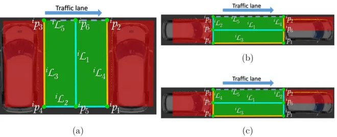
3.1 Parking spot models for non-parallel (b) and parallel (backward (b) and forward (c)) parking maneuvers . . . 44 3.2 Weighting function wt

i . . . 45

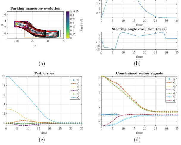
3.3 Example of what different features used as constraints for collision avoid-ance mean physically. . . 47 3.4 Backward ⊥ parking maneuver signals: (a) performed maneuver (θT =0 = 5),

(b) control signals, (c) task error signal, (d) constrained sensor signals . . . 54 3.5 Backward ⊥ parking maneuvers. (a) θT =0 = 25°. (b) θT =0 = 30° . . . 54

3.6 Backward diagonal parking maneuver signals: (a) performed maneuver (ini-tial pose = (6.7 m, 7.5 m, 0°)), (b) control signals, (c) task error signal, (d) constrained sensor signals . . . 55 3.7 Backward diagonal parking maneuvers. (a) Initial pose = (6.1 m, 7.5 m, 0°).

(b) Initial pose = (6 m, 7.5 m, 0°) . . . 56 3.8 Forward perpendicular parking maneuver signals: (a) performed maneuver

(initial pose = (−9 m, 10.5 m, 0°)), (b) control signals, (c) task error signal, (d) constrained sensor signals . . . 57 3.9 Forward perpendicular parking maneuvers. (a) Initial pose = (−9 m, 8.1 m,

0°). (b) Initial pose = (−13.5 m, 8.1 m, 0°) . . . 57 3.10 Forward diagonal parking maneuver signals: (a) performed maneuver

(ini-tial pose = (−5.6 m, 7.4 m, 0°)), (b) control signals, (c) task error signal, (d) constrained sensor signals . . . 58 3.11 Forward diagonal parking maneuvers. (a) Initial pose = (−5.6 m, 6 m. 0°).

(b) Initial pose = (−5.6 m, 9 m, 0°) . . . 59 3.12 Backward k parking maneuver signals: (a) performed maneuver (initial

pose = (9.5 m, 2.5 m, 0°)), (b) control signals, (c) task error signal, (d) constrained sensor signals . . . 60 3.13 Backward k parking maneuvers. (a) Initial pose = (8.2 m, 5 m, 0°). (b)

Initial pose = (6.5 m, 3 m, 0°) . . . 60 3.14 Forward k parking maneuver signals: (a) performed maneuver (initial pose

= (−10 m, 3 m, 0°)), (b) control signals, (c) task error signal, (d) con-strained sensor signals . . . 61 3.15 Forward k parking maneuvers. (a) Initial pose = (−12.3 m, 3 m, 0°). (b)

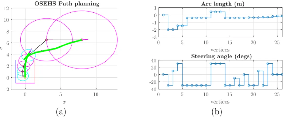
3.16 OSEHS Path planning approach results: three maneuvers are required. Ini-tial pose = (8m, 6.5m, 5°) . . . 63 3.17 OSEHS Path planning approach results: three maneuvers are required.

Ini-tial pose = (5m, 6.5m, 0°). . . 63 3.18 Exhaustive simulations for different types of parking maneuvers with a

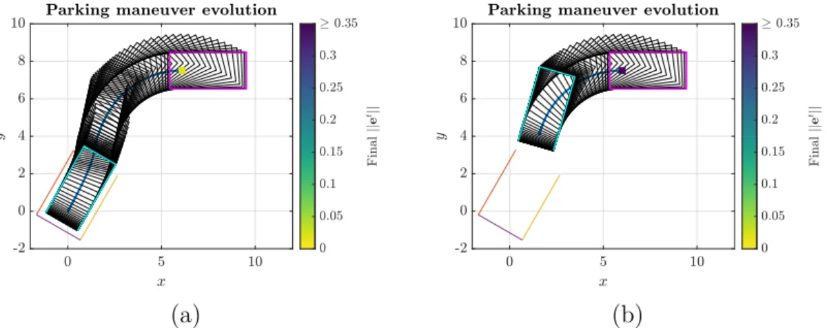
sampling step of 10cm for the initial position. For non-parallel cases: spot length = 4 m and width = 2.7 m. For (e): spot length = 7.5 m and width = 2.3 m. For (f): spot length = 11.5 m and width = 2.3 m. The color indicates the final error norm, ranging from dark blue for values above 0.35 (typically above ≈ 35 cm in position) to pure yellow for values below 0.03 (typically below ≈ 3 cm in position). . . 65 3.19 Forward ⊥ unparking maneuver signals: (a) performed maneuver (desired

pose = (5 m, 6.5 m, 0°)), (b) control signals, (c) task error signal, (d) con-strained sensor signals . . . 66 3.20 Forward ⊥ unparking maneuvers. (a) Desired pose = (6.5 m. 6.5 m, 0°), (b)

Desired pose = (6.5 m, 6.5 m, −10°) . . . 67 3.21 Forward diagonal unparking maneuver signals: (a) performed maneuver

(desired pose = (5.5 m, 4.2 m, 0°)), (b) control signals, (c) task error signal, (d) constrained sensor signals . . . 68 3.22 Forward diagonal unparking maneuvers. (a) Desired pose = (5.5 m, 7.5 m,

0°), (b) Desired pose = (7 m, 7.5 m, 0°) . . . 68 3.23 Backward ⊥ unparking maneuver signals: (a) performed maneuver (desired

pose = (−5.4 m, 10 m, 0°)), (b) control signals, (c) task error signal, (d) constrained sensor signals . . . 69 3.24 Backward ⊥ unparking maneuvers. (a) Desired pose = (−5.4 m. 8.1 m, 0°),

(b) Desired pose = (−9 m, 8.1 m, 0°) . . . 70 3.25 Backward diagonal unparking maneuver signals: (a) performed maneuver

(desired pose = (−6 m, 7.5 m, 0°)), (b) control signals, (c) task error signal, (d) constrained sensor signals . . . 71 3.26 Backward diagonal unparking maneuvers. (a) Desired pose = (−6 m. 5.5 m,

0°), (b) Desired pose = (−9 m, 5.5 m, 0°) . . . 71 3.27 Exhaustive simulations. Final orientation = 0°. Parking spot length = 4 m

3.28 Forward perpendicular unparking maneuver in simulation using a home-made fast prototyping environment . . . 73 3.29 Forward perpendicular unparking maneuver signals . . . 74 3.30 Experimental car parking in a perpendicular spot using online feature

ex-traction . . . 75 3.31 Backward ⊥ case, spot length = 4 m and width = 3 m. Initial

orienta-tion = 1.35° . . . 75 3.32 Real backward ⊥ parking maneuver signals . . . 76 3.33 Experimental car parking in a perpendicular spot . . . 77 3.34 Backward ⊥ case, spot length = 4.5m and width = 2.85m. Initial

orienta-tion = 176° . . . 78 3.35 Real backward ⊥ parking maneuver signals . . . 78 4.1 Parking spot models for backward (a) and forward (b) non-parallel types

and for (c) parallel ones . . . 83 4.2 Example of a parking environment. The green rectangle denotes the parking

spot into which the car should park. Red areas are considered forbidden zones, as such the vehicle should never go into them. Furthermore, it is considered that parking maneuvers can only start inside the transitable area and if no portion of the vehicle is inside any of the forbidden zones while unparking maneuvers can only start if the vehicle is in a parked pose (i.e. inside a parking spot). . . 85 4.3 Control structure [63] . . . 90 4.4 Generic weighting function w(s) . . . 93 4.5 Constrained ⊥ backward parking maneuver signals: (a) performed

maneu-ver, (c) control signals, (e) weighting-related signals, (b) main and (d) aux-iliary task errors and (d) constrained sensor signals. Initial pose = (8 m, 6 m, 0°) . . . 97 4.6 Constrained ⊥ backward parking maneuvers. (a) Initial pose = (8 m, 7.5 m,

−5°), (b) Initial pose = (0 m, 5.1 m, 0°) . . . 98 4.7 Constrained diagonal backward parking maneuvers. (a) Initial pose = (8 m,

6 m, 0°), (b) Initial pose = (0 m, 5.1 m, 0°) . . . 99 4.8 Constrained non-parallel forward parking maneuvers: (a) diagonal and (b)

4.9 Constrained k backward parking maneuvers. (a) Initial pose = (0.5 m,

2.7 m, 0°), (b) Initial pose = (8 m, 2.5 m, 0°) . . . 100

4.10 RRT∗ _{path planning results using HC}00 _{steering function. Initial pose =} (8m, 6m, 0°) . . . 101

4.11 RRT∗ _{path planning results using HC}00 _{steering function. Initial pose =} (8m, 7.5m, −5°) . . . 102

4.12 RRT∗ _{path planning results using HC}00_{-RS steering function. Initial pose} = (0m, 5.1m, 0°) . . . 102

4.13 Exhaustive simulations for different types of parking maneuvers with a sampling step of 20 cm for the initial position. For non-parallel cases: spot length = 5 m and width = 2.7 m. For (e): spot length = 5.6 m and width = 2 m. . . 103

4.14 Constrained ⊥ backward parking maneuver with a moving obstacle travel-ing from right to left . . . 105

4.15 Constrained ⊥ backward parking maneuver with a moving obstacle travel-ing from top to bottom . . . 106

4.16 Constrained ⊥ backward parking maneuver with a moving obstacle travel-ing from left to right . . . 107

4.17 Constrained ⊥ backward parking maneuver with an obstacle blocking the entrance of the parking spot at the beginning . . . 108

4.18 Constrained ⊥ backward parking maneuver with a child playing around the mother . . . 109

4.19 Constrained k forward unparking maneuver signals: (a) performed maneu-ver, (c) control signals, (e) weighting-related signals, (b) main and (d) aux-iliary task errors and (d) constrained sensor signals. Desired pose = (8 m, 2.5 m, 0°) . . . 111

4.20 Constrained k forward unparking maneuvers. (a) Desired pose = (2.5 m, 4.7 m, 0°), (b) Initial pose = (6.7 m, 3.5 m, 0°) . . . 112

4.21 Exhaustive simulations for forward parallel unparking maneuvers with a sampling step of 20 cm for the initial position. Spot length = 5.6 m and width = 2 m . . . 113

4.22 Experimental car parking in a perpendicular spot . . . 114

4.23 Constrained real backward ⊥ parking maneuver signals . . . 114

4.25 Constrained real backward k parking maneuver signals . . . 115 4.26 Experimental car unparking from a parallel spot . . . 116 4.27 Constrained real forward k unparking maneuver signals . . . 116

2.1 Dimensional vehicle parameters . . . 33

3.1 Pair of points through which each line passes . . . 44

3.2 Control-related vehicle parameters . . . 53

4.1 Pair of points through which each line passes . . . 82

4.2 Control-related vehicle parameters . . . 96

A.1 Constraints deactivation - backward non-parallel case . . . 125

A.2 Constraints deactivation - forward non-parallel case . . . 125

A.3 Constraints deactivation - backward parallel case . . . 125

A.4 Constraints deactivation - forward parallel case . . . 126

A.5 Constraints deactivation conditions - forward non-parallel case . . . 127

A.6 Constraints deactivation conditions - backward non-parallel case . . . 127

B.1 Constraints deactivation - backward non-parallel case . . . 129

B.2 Constraints deactivation - forward non-parallel case . . . 130

B.3 Constraints deactivation - backward parallel parking / forward parallel unparking . . . 131

Vehicles and Intelligent Transportation systems have followed a quick mutation thanks to the growing use of electric technology and the emergence of autonomous navigation techniques. So much so that the hype created around self-driving vehicles even lead parts of the industry to overestimate their arrival [1] as commercial products. Even if often overlooked when talking about autonomous driving, the amount of maneuvering that encompass the different tasks that a driver would perform in a parking scenario (look for an empty parking spot, park, unpark, etc.) - even more so in crowded places, contribute in no small part to the complexity of developing a fully autonomous driving system [2].

In [3] it is estimated that 30% of the traffic in any city is people in cars searching for parking. A different study [4] says that 45% of total traffic on 7th Avenue in Brooklyn is

people looking for a parking space. According to [5], the burden of finding a free parking spot can be such that 100% of car owners in a couple of districts of Paris have abandoned their trip at least once. The statistics of a survey carried by the University of Michigan

Transportation Research Institute shows that about 10,000 of 12 million traffic accidents

occur while entering or leaving parking lots although it is affirmed that the actual num-ber of parking related accidents is much more than the reported numnum-ber [6]. Currently commercially available parking assistance systems, using mainly cameras and ultrasonic sensors to perceive the environment, have lead to a significant increase of driving comfort and provided cost savings from (avoidance of) accidents [7]. It is clear that advanced Intelligent Parking Systems would be of great use.

Even if many car manufactures already offer the first generation of automatic parking systems, it is still necessary to imagine the new generation. The most complete solution for the parking problem, and the dream of many, would be to be able to, once the driver arrives to the desired destination, leave the car at the entrance of the building or at the entrance of a dedicated parking lot (if any) and forget about it, letting the car park by it-self safely and autonomously in an available (parallel, perpendicular or diagonal) parking spot (Figure 1a) and, whenever the user wants leave, be able to summon the car remotely to go to the driver’s location and pick him/her up (Figure 1b). Therefore, the new gen-eration of Intelligent Parking Systems requires the implementation of different advanced

(a) Car parking autonomously

(b) Car unparking autonomously

Figure 1: Autonomous Parking - Volvo Cars Innovations [8]

functionalities: move and look for an empty place autonomously in an encumbered envi-ronment, check the parking maneuver compatibility, perform the parking and unparking maneuvers, navigate autonomously from the parking spot to the place to pickup the user and obviously to communicate with the user and the parking exploitation company.

The mobile robotics research axe of the LS2N’s ARMEN team is involved on the devel-opment of autonomous vehicles applications. As part of its efforts, the team participates in the ANR project VALET. This project studies a full Valet Parking System to be im-plemented at a city level. Thus, the work done during the PhD falls under the umbrella of the ANR project VALET, aiming to address the parking related tasks.

As such, the main objective of the PhD is to revisit the tasks of parking and other maneuvers with the multi-sensor based approach - an approach that has proven its efficacy and robustness in many different robotic applications, and compare them with already existing approaches. In order to attain the objectives it is necessary to understand the nonholonomic constraints inherent to car-like robots and the implications they have when doing path planning - a typical approach followed in the literature for solving motion problems, or while controlling the vehicle. Moreover, since (as the name implies)

sensor-based control approaches rely heavily on the sensor information available, the perception problem has to be taken into account. Regarding the control problem, a common approach in robotics is to make use of the task function approach [9] which allows to specify the task to be performed as an output function associated to the state equation of the robot. Nevertheless, due to safety and comfort reasons, control techniques that are capable of ex-plicitly dealing with constraints, such as Model Predictive Control (MPC), are of interest for our application.

Thanks to the work done during the PhD thesis, two different frameworks were devel-oped. The first framework, using a Multi-Sensor-Based Control (MSBC) approach, allows to formalize different parking and unparking operations in a single maneuver with either backward or forward motions. Building upon the first one and by using an MPC strategy, a Multi-Sensor-Based Predictive Control (MSBPC) framework was developed, allowing the vehicle to park autonomously (with multiple maneuvers, if required) into perpendicu-lar and diagonal parking spots with both forward and backward motions and into parallel ones with backward motions in addition to unpark from parallel spots with forward mo-tions. These frameworks have been tested extensively using a robotized Renault ZOE with positive outcomes and now they are part of the autonomous driving architecture being developed at LS2N.

In the first chapter an overview of the state-of-the-art parking techniques is presented, followed by related works on sensor-based control applied to car-like robots, an introduc-tion and key aspects of Model Predictive Control (MPC) strategies and an overview of the relevant perception systems for intelligent vehicles. Chapter 2 introduces the modeling and notation for car-like robots and the multi-sensor framework as well as the considered perception system. The following chapter presents the work done on the MSBC approach for performing parking and unparking operations in a single maneuver. The MSBPC for parking in multiple maneuvers is presented in Chapter 4. Finally, general conclusions and perspectives for future work are discussed.

Publications

Journal Articles

D. Pérez-Morales, O. Kermorgant, S. Domínguez-Quijada, and P. Martinet, “Multi-Sensor-Based Control For Autonomous Parking”, IEEE Transactions on Intelligent Vehicles.,

Submitted, 2019.

Conference Proceedings

D. Pérez-Morales, O. Kermorgant, S. Domínguez-Quijada, and P. Martinet, “Automatic Perpendicular and Diagonal Unparking Using a Multi-Sensor-Based Control Approach”,

in 2018 15th International Conference on Control, Automation, Robotics and Vision,

Singapore, Singapore: IEEE, Nov. 2018, pp. 783–788.

D. Perez-Morales, O. Kermorgant, S. Dominguez-Quijada, and P. Martinet, “Laser-Based Control Law for Autonomous Parallel and Perpendicular Parking”, in Second IEEE

International Conference on Robotic Computing, Laguna Hills, USA, 2018, pp. 64–71.

Peer-reviewed workshops

D. Pérez-Morales, O. Kermorgant, S. Domínguez-Quijada, and P. Martinet, “Multi-Sensor-Based Predictive Control for Autonomous Backward Perpendicular and Diagonal Park-ing”, in 10th Workshop on Planning, Perception and Navigation for Intelligent Vehicles

at IEEE/RSJ IROS, Madrid, Spain, 2018.

——, “Autonomous Perpendicular And Parallel Parking Using Multi-Sensor Based Con-trol”, in 9th Workshop on Planning, Perception and Navigation for Intelligent Vehicles

Related work

In this chapter an overview of the work related to Intelligent Parking applications is presented. We start by defining the relevant classifications that exist in the literature to categorize self-driving cars in general and Parking and Maneuvering Assistance Systems (PMAS) in particular as well as an overview of the current industrial state. Afterwards, we review the state-of-the-art on parking techniques with a particular focus on path planning approaches - a popular choice in recent years. Then, the basic concepts of sensor-based control are introduced as well as the few works available on the literature applied to car-like robots. Then, the basics of Model Predictive Control (MPC) strategies and their essential properties are given as well as some examples of applications exploiting predictive techniques followed by a key framework that combines sensor-based control (i.e. Visual Servoing (VS)) and MPC strategies. Finally, the perception issue is briefly introduced alongside an overview of the key characteristics of the different sensors typically considered for autonomous vehicles.

1.1

Relevant classifications

When talking about self-driving cars, probably the two most relevant classifications that appear in the literature are, on the one hand, the one provided by SAE International [10] and, on the other hand, the one given by the International Organization of Motor Vehicle

Manufacturers (OICA by its French acronym) [11], with the latter being based on the

former. Both define six levels of automation (from level 0 to 5) where the lower level is used to define a driver only level (i.e. no active systems are involved) while the highest one (level 5) is used to denote full automation - the vehicle is able to drive itself under all conditions with no human intervention. When the vehicle is able to control either the longitudinal or the lateral motion of the vehicle one is talking about a system of level 1 but if the car is able to perform both tasks one refers to level 2 or higher. The difference between the higher levels (2 and above) lies on the requirement (or lack of thereof) of a

driver with level 2 requiring the driver to supervise the vehicle at all times while level 3 requiring the driver to be in position to retake control of the vehicle (if the system deems it necessary) but not actively supervising it. As for the fourth level, no driver is required in defined use cases.

Considering that our application has a well defined scope, the classification of Parking and Maneuvering Assistance Systems (PMAS) defined in the Handbook of Intelligent Vehicles [7] is of relevance as well. In this one, two main categories are defined: Passive and Active systems.

Passive PMAS refer to those that do not interact with the actuators of the vehicle (i.e they do not perform any control) but rather are used to warn the driver about nearby objects, inform if a given parking spot is suitable for the vehicle or provide video feeds from one or multiple cameras (often with auxiliary lines superimposed) to help the driver to best steer the vehicle into the parking spot. As the reader might have already guessed, passive PMAS overlap with the level 0 of driving automation defined above.

Regarding active PMAS, there are three subcategories: semiautomatic, fully automatic and autonomous parking assistance. Similarly to the previously defined levels of driving automation, the difference among these systems lies on the level of involvement of the driver.

Semiautomatic parking assistance overlaps with level 1 systems since this type of systems only control the steering wheel while the driver has to control the longitudinal motion of the vehicle. To the best of my knowledge, the first commercial offer of this type of assistant was made by Toyota on 2003 in Japan under the name of Intelligent Parking Assist. [12]. Many other car manufacturers (Ford, Lincoln, PSA Peugeot Citroën, BMW, Volkswage, Nissan, Mercedes-Benz, Land Rover, among others) [13] [14] [15] currently offer (or had offered) this type of systems.

Fully automatic systems refer to those that are capable of performing the whole parking maneuver but, depending on whether or not the driver is expected to actively supervise the vehicle, they can be part of either level 2 or 3 systems. The first commercial offers were provided by BMW [16] and Tesla Motors [17]. Many other manufacturers have working prototypes.

The most advanced subcategory, autonomous parking assistance, refers to systems that do not require human intervention nor supervision and, depending on whether they can work under any circumstance or only for defined use cases they can be considered either level 5 or 4 systems. Currently there are no commercial offers that have reached

this category although Audi [18], BMW [19] and Tesla Motors [20] have shown working prototypes. It should be noted that, Tesla’s situation on this regard is a special case given that they have early access programs for some of their features such as Enhanced Summon [2] thus being (to some extent) commercially available but not considered as a finished feature.

1.2

State-of-the-art parking techniques

As it can be seen in [6], the literature related to automatic parking is quite extensive, having many different control approaches available. Despite the fact that the automobile industry has already started to roll out some commercial implementations of active park-ing assistants capable of actively controllpark-ing acceleration, brakpark-ing and steerpark-ing [21], the research interest in the topic remains strong.

The different control approaches available in the literature can be divided into two categories [22]: one based on stabilizing the vehicle to a target point, with fuzzy con-trol being the most widely investigated from this category and with one of the earliest works on automatic parking [23] using sinusoidal control functions; the other is based on path planning, where geometric collision-free path planning approaches based on the non-holonomic kinematic model of a vehicle have been of special interest in recent years [24]–[26]. Relatively typical parking control theories are fuzzy control, neural network con-trol and concon-trol method based on linear inequalities [6]. As for combined planned/reactive approaches, a pioneering work in the matter is reported in [27], where a behavior based architecture is used to combine the contributions of the different planned and reactive behavior towards a common goal: parking while avoiding collision.

In [28] a neuro-fuzzy sensor based controller is presented. The controller is able to decide about the motion direction at each time interval by processing the information obtained from the sensors. The key idea of their scheme is to construct a mapping between sonar sensors measurements and the turning angle in order to plan and carry out the sensor based maneuvers required for parking and, since the mapping is directly established between the sensor measurements and the turning angle there is no need to deal with radial imprecision and angular uncertainty.

In [29] a technique for integrating metric and semantic maps for vision-only automated parking is reported. Said maps are built and maintained using the data obtained from the cameras mounted on the car. In the semantic maps, two types of semantic labels are

considered: static and dynamic. From those maps, the car used to collect the data to build them, was able autonomously drive inside the parking lot and park in a predefined parking slot with a relatively good accuracy, although the approach used to realize the parking tasks is not specified.

Expanding slightly the scope of the state-of-the-art, one can find works on docking of electric cars for recharging purposes [30] as well as for academic mobile robots [31]. In [30], the pose of the vehicle is reconstructed using a infrared perception system and a known infrared pattern on the charging base in order to stabilize the pose of the vehicle at the desired value. As for [31], a given path is deformed in a reactive fashion using sensor data in order to avoid collision and/or to reach a desired (perceived) docked pose; experimental results have been shown for collision avoidance and docking using a differential mobile robot towing a cart [31] and, using the same approach, collision avoidance results have been shown for a car-like robot in [32].

As show in [33], path planning approaches for automated vehicles have been heavily investigated in recent years.

In [34] and [25] techniques to perform, respectively, parallel and parking maneuvers where the path planning step is addressed by a combination of admissible collision-free circulars arcs and tangent straight lines are presented. In both techniques, the problem of stabilizing the vehicle at a desired position and orientation is seen as an extension of the path tracking problem. Saturated controllers are proposed to achieve a quick steering without chattering when performing the parking maneuvers.

Following similar geometric principles, the approach reported in [35] relies on three sub-paths: two circles and a straight line, each one tangent to the next one. This work addresses forward and backward perpendicular parking maneuvers and backward parallel ones.

A path planning approach that considers clothoids (a curve whose curvature varies linearly with its arc length) for parking into parallel spots, for both forward and backwards motions, can be found in [26]. The use of clothoids is considered in order to account for the limitations on the steering velocity of the vehicle, answering to the admissibility constraints of car-like vehicles.

Similarly, to plan smooth paths, in [36] the authors make use of clothoid-like curves. Parking into non-parallel parking spots, in addition to parallel ones was considered in this work although only for backward maneuvers.

in [37]. The authors localize the vehicle in a known environment by means of vision approaches while the obstacle detection is performed using ultrasonic sensors. Inside this environment, the car is able to park autonomously in a previously taught parked pose from a learned (or in the vicinity of it) departure position. If the vehicle finds itself out of the known path, new local paths that bring the vehicle to the usual one are computed using geometric methods like the ones reported in [38].

The heuristic exploration-based planning approach reported in [39] makes use of the knowledge of the vehicle’s orientation during the exploration phase in order to improve the planning efficiency in maneuvering scenarios when compared to common random-sampling methods and general heuristic search methods. The (rather short) computation time claimed by the authors could allow this technique to be used for online replanning. From the RRT-based path planning approaches, one can highlight [40]–[42]. These three works use the same BiRRT∗ _{backbone planner with the difference being on how the}

sampling is guided. In [40] a Hybrid Curvature (HC) steering function based on clothoids is introduced in order to ensure continuity on the steering angle while the vehicle is moving in one direction but allows curvature discontinuities where a change of (longitudinal) di-rection occurs. In order to ensure that the curvatures respect the actuator limits regarding the maximum acceleration, in [41] the sampling is guided using Hybrid Curvature Rate (HCR) steering functions. The HCR steering function is based on cubic spirals. Finally, in [42] the sampling is guided by a Convolutional Neural Network (CNN). In this case, the CNN has been trained with simulated data. Its goal is to predict the future poses of the vehicle given the current driving situation in order to guide the planner towards an optimal solution.

An (often) overlooked point is that, solving the motion planning problem does not equal to solving the maneuvering one. Due to the nonholonomic constraints that the ve-hicle is subject to, small discrepancies between the model and the real platform, noise in the sensor measurements, localization errors, external disturbances, etc. could poten-tially produce non-negligible discrepancies between the planned path and the actual path performed by the vehicle, especially as the amount of changes of longitudinal direction increases.

Taking as an example Fig. 1.1 one can consider the planning problem to be addressed successfully and, looking at the simulations results (Fig. 1.1a), the maneuvering problem seems to be solved as well but, when one looks at the experimental results (Fig. 1.1b) it is clear that the vehicle doesn’t follow exactly the planned path. Similar outcomes can

be seen in Fig. 1.2 where the discrepancies between the planned and the actual path are non-negligible.

(a) (b)

Figure 1.1: Results presented in [36]: (a) simulations and (b) real experimentation

(a) (b)

Figure 1.2: Real experimentation results presented in [26]: (a) parking in four maneuvers, (b) parking in one and two maneuvers

1.3

Sensor-based control applied to car-like robots

(a) Sensor data are used to estimate

the position of the robot (b) Sensor data are directly inte-grated in the control loop Figure 1.3: Block diagrams of (a) classical position control and (b) multi-sensor-based control

Contrary to the original use of sensors in classical position control where their data are used to provide position feedback (Fig. 1.3a), sensor-based control techniques integrate the sensor data directly in the control loop (Fig. 1.3b). As such, is not the robot anymore that should reach a given desired position but instead is the sensor that should perceive a given desired value (e.g. a camera that should view a certain image, an ultrasonic sensor that should measure a given desired distance, etc.).

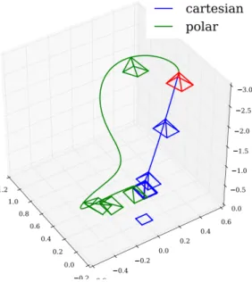
Sensor-based control techniques based on the task function approach [9] (i.e. VS [43], [44]) have proven its efficacy in many robotics applications (manipulation, grasping, par-allel robotics, mobile robotics, etc.) although few works are available in the literature on car-like robot applications. A key benefit of these techniques is their great robustness against modeling and calibration errors, particularly when then pose of the robot doesn’t need to be reconstructed (i.e. Image-Based Visual Servoing (IBVS)) and, since they rely only in locally perceived information, they do not suffer from localization issues. On the contrary, given that the task is expressed in the sensor space, the trajectory of the robot depends heavily on the choice of sensor features and parametrization (Fig. 1.4), therefore it is difficult to predict its behavior without testing it beforehand.

A visual servoing approach for path reaching and following is reported in [45] requiring only a few path features. Real experimentation using a car-like robot and comparisons between Position-Based Visual Servoing (PBVS) and IBVS are presented, showing that, if the control law is well designed and the features remain visible, the IBVS approach is gen-erally better, having smoother control signals and being more robust against calibration errors.

Figure 1.4: Trajectories of a flying camera using an image point as the sensor feature parameterized using Cartesian and polar coordinates

In [46] the navigation task of the car-like robot is performed autonomously using vision while avoiding the obstacles detected by a 2D LiDAR. The path to follow consist of an ordered set of key images that have been previously acquired during the teaching phase. In an attempt to minimize the issues caused by degraded localization performance in urban environments, sensor-based control approaches have been recently investigated in the context of navigation [47] and dynamic obstacles avoidance [48].

Regarding maneuvering tasks (e.g. parking, unparking, half turn), few things have been investigated [49].

1.4

Model Predictive Control

The term Model Predictive Control (MPC) does not refer to a specific control strategy but rather to a wide variety of control methods that explicitly use a model of the pro-cess in order to obtain the control signal by minimizing an objective function [50]. The origins of this type of strategies can be tracked back to [51], initially proposed for indus-trial processes. MPC is considered a mature strategy for linear and slow systems while nonlinear, hybrid or very fast processes were considered beyond the realm of MPC in no small part due to computational demands. Nonetheless, thanks to advances in computing capabilities and the associated cost reduction, MPC techniques have been investigated

for many different (previously considered as unfeasible) applications in recent years [52] -e.g. automotive, health care, finance, etc.

The basic ideas of this type of techniques are to explicitly use a model to predict the output of the process at future time instants up to a given horizon, the computation of control sequence that minimizes a given objective function and the use of a receding strategy in order to displace the horizon towards the future and, at each step applying the first control signal of the computed sequence (Fig. 1.5).

Figure 1.5: Temporal diagram of the finite-horizon prediction [53]

A key benefit of MPC strategies is that, when using a finite-horizon, it is possible to explicitly handle constraints on the states, inputs and outputs. On the contrary, from a theoretical point of view, when using a nonlinear model the control problem is a non-convex Non-Linear Program (NLP) thus the solution is rather complex and there is no guarantee that the global optimum can be found [50].

In spite of the challenges that nonlinear problems pose for MPC strategies, for differ-ential mobile robots, such techniques have been proven to be feasible for stabilizing the robot at a desired pose [54] and for performing trajectory tracking [55]. Furthermore, in [56] it was shown that it is possible to generate a reactive walking pattern for a humanoid robot in real time using a Nonlinear Model Predictive Control (NMPC) strategy.

In [57]–[59] predictive strategies were developed to compensate for the delay in the response of the steering angle of off-road car-like vehicles when following a given path by exploiting the knowledge of future curvature values along the path. A single robotized

tractor was used to validate the approach in [57], [58] while in [59] multiple robots in a given (potentially varying) formation were considered.

In recent years the use of MPC as part of Artificial Intelligence (AI) algorithms has been investigated [60], [61]. In [60] an efficient (both in computation time and memory usage) differentiable MPC is presented and used as a policy class for reinforcement and imitation learning. As for [61], based on an MPC strategy, the dynamics of the agent are learned with a model-based reinforcement learning algorithm and afterwards the learned dynamics are used to initialize a model-free learner to improve the final results. The authors claim that the hybrid approach is able reach comparable results to purely model-free learners but requiring significantly less samples.

Regarding the choice of the control horizon, it has been shown in [62] that, for a car-like robot described in natural coordinates, the minimal control horizon required in order to control its full state has to be equal to 3 (equal to the degree of nonholonomy - 1).

The framework presented in [63] formalizes the IBVS subject to constraints (workspace limitations, visibility constraints and actuator limitations) with a predictive control strat-egy by writing the IBVS task as a nonlinear optimization problem. On the one hand, thanks to the predictive strategy, the different considered constraints can be explicitly handled. On the other hand, the well-known robustness against noise and modeling errors of sensor-based control techniques is preserved as well as the local asymptotic stability property of such type of approaches. Additionally, it is shown that a local model based on the interaction matrix is enough to predict the evolution of the sensor features and thus allows to perform successfully VS tasks while satisfying the considered constraints. Given that this framework links MPC and sensor-based control strategies, it will be key for the development of Chapter 4 where a novel approach for performing parking/unparking maneuvers (starting from virtually any initial position in the workspace) in a reactive fashion is presented.

1.5

Perception

In order to perceive the environment, autonomous vehicles have to be equipped with several sensors. The most relevant types of exteroceptive sensors for intelligent vehicles (Fig. 1.6) are radar, laser, vision and ultrasonic [64]. Each type of sensors has different inherent characteristics and price points that make them more or less suitable for certain tasks.

(a) Radar (b) Laser

(c) Ultrasonic (d) Vision

Figure 1.6: Examples of exteroceptive sensors for intelligent vehicles

Radars can provide information about the distance, velocity and angle of detection of perceived objects. These type of sensors are in general rather robust against adverse weather conditions and the detection range (at least for long-range radars) is often the longest (up to 200 m) although the Field Of View (FOV) is often very narrow.

Laser scanners or Light Detection And Ranging (LiDAR)s take measurements accord-ing to the time-of-flight principle. The detection range for this type of sensors is usually around 100 m although the newest versions are capable of reaching 300 m. The lateral reso-lution and FOV is considerably better for this sensors than for radars although in general are less robust against adverse weather conditions. With enough layers, the amount of detail provided can rival vision systems (not considering the color) although increasing layers usually means a rather significant increase in price. Often in both academic and industrial research setups, the LiDARs used have moving parts to achieve a lager hori-zontal FOV (i.e. rotating LiDARs) although recently developed solid sate LiDARs aim to improve the durability of the sensor and reduce its cost at the expense of FOV [65].

Ultrasonic sensors are the most widely adopted in the industry because of their low cost, lightweight, low power consumption and low computation requirements compared to other ranging sensors. On the other hand they have the shortest range and are able only to tell whether or not there is an object in the detection range and at which distance

with no information on the angle, size or shape.

Vision systems are getting more popular in the industry as time goes by due to their reasonable cost and the amount of information they can provide, allowing to detect and classify traffic signs, pedestrians, vehicles, etc. Depending on the type of wavelength per-ceived, cameras can be classified as visible (VIS) or infrared (IR) for passive ones or as (active) Time-of-Flight (ToF) if the system uses the time-of-flight principle to measure distance by emitting near infrared (NIR) light pulses [65]. Nevertheless, the amount of information comes at the cost of relatively high computational processing requirements. Depending on the task to accomplish one could consider monocular vision systems (mostly for detection and classification) or stereo vision systems when depth information is re-quired and the range of ToF is not enough. The performance of these systems is often very dependent on the environment and visibility conditions.

The key characteristics of different sensors typically used in intelligent vehicles ap-plications are well summarized in [65] (Fig. 1.7) and compared against a perfect sensor. It can be clearly seen that no sensor can be considered perfect although the closest one, depending on the perception requirements, could be argued to be VIS cameras with both LiDAR variants following closely.

Regarding the perception algorithms available in the literature to extract parking spots from sensors embedded in the vehicle, we now give an overview of different works using different (combinations) of sensors.

Having knowledge of the parking area stored in a digital map - including parking spots, the authors of [66] simply use the sensor data (four 2D LiDARs) to build an occupancy grid. Using this occupancy grid and an occupancy Bayes’ formula, the state (free or occupied) of a given parking spot is determined.

Considering a system where the user selects the desired parking spot by touching a display showing a rear view image, the authors of [67] define a Region Of Interest (ROI) in which the system looks for a parking spot. The parking spot is extracted from a bird’s-eye view using a Hough transform.

In [68] an algorithm that fuses vision data from a bird’s-eye view (built from four cameras, one on each side of the vehicle) and ultrasonic sensors is reported. The work focuses on the detection and tracking of parking spots in underground and indoor envi-ronments. Due to this, only rectangular parking spots are considered. Additionally, pillar information (typical in such environments) is exploited to improve the performance of the approach.

FOV Range Accuracy Frame rate Resolution Color perception Size Weather affections Maintenance Visibility Price ToF IR VIS Perfect sensor (a) Cameras FOV Range Accuracy Frame rate Resolution Color perception Size Weather affections Maintenance Visibility Price Solid state Rotating Perfect sensor (b) LiDAR FOV Range Accuracy Frame rate Resolution Color perception Size Weather affections Maintenance Visibility Price RADAR Perfect sensor (c) RADAR FOV Range Accuracy Frame rate Resolution Color perception Size Weather affections Maintenance Visibility Price Ultrasonic Perfect sensor (d) Ultrasonic

Figure 1.7: Comparison of the main features of different sensors typically used in intelligent vehicles according to [65].

Using as well bird’s-eye view images, in [69] an algorithm capable of recognizing free parking spots of any type (perpendicular, diagonal and parallel) is presented. The authors use a height map constructed by means of dense motion-stereo vision in order to distin-guish between road and obstacles. To extract the road markings, which are assumed to have a fixed thickness, a probability map with a salient feature is used and, finally, the parking spot recognition is performed by means of a Bayesian classifier.

Using 2D LiDAR information, [70] presents an algorithm capable of extracting and tracking empty perpendicular parking spots from the free space between two detected vehicles. The authors assume that the already parked vehicles have an L-shape and as such, they use rectangular and round corner detection as the basis of the approach.

In [71], the data of a 3D LiDAR with 32 layers is used to map the environment using a Simultaneous Localization and Mapping (SLAM) approach. From this map, the already parked vehicles are extracted using a CNN. By fusing the map and the detected vehicles, the authors estimate the topology of parking lots and infer vacant parking spots in a graph-based approach.

1.6

Conclusion

Following the classifications introduced in this chapter, we are aiming to reach a level 4 and therefore an autonomous parking assistance system level although, considering that the work done during the PhD thesis was focused on the control issue, for the most part, we depend on external perception algorithms in order to tell whether or not our system is actually able to reach the desired level.

Regarding the overview of the state-of-the-art parking technique, an often overlooked point has been identified when working with nonholonomic mobile robots: solving the motion planning problem does not equal to solving the maneuvering one.

We have also seen that, in spite of the interesting properties that sensor-based control approaches bring to the table and the fact that it has been proved effective in many different robotic applications, few work has been done on car-like robot applications. Additionally, a key framework that combines sensor-based control and MPC strategies [63] was introduced.

Regarding the perception issues, we have introduced most relevant exteroceptive sen-sors for intelligent vehicles applications as well as the main benefits and drawbacks of each of them. Furthermore, some works on parking spot extraction using different (com-binations of the) sensors considered were presented.

Modeling and notation

In this chapter we define the modeling considered for the car-like robot as well as the multi-sensor-based modeling formalism which later will allow to define the required task and constrained sensor features and explain how they relate to the vehicle’s velocity. Additionally, the perception system configuration is defined, an example of how an empty parking spot could be extracted from the sensor data is given as well as how, by using virtual sensors the definition of the different sensor features can be more direct. Finally, the parametrization used for modeling straight lines (crucial for our application) is given.

2.1

Car-like robot model and notation

Given that parking applications are generally executed at low-speed motions, a kinematic model can be considered as accurate enough.

For the sake of clarity, for the equations and explanations presented in this work, the parking spot is considered to be always on the right side of the vehicle to park at the beginning of the maneuver. Furthermore, all the sensors are assumed to be calibrated.

Considering the well-known kinematic model of a car with rear-wheel driving [72]:

         ˙x ˙y ˙θ ˙φ          =          cos θ sin θ tan φ/lwb 0          vxm+          0 0 0 1          ˙φ, _(2.1)

the vehicle’s twist is defined by the following column vector (elements separated by a semicolon):

vm = [vxm; ˙θm], (2.2)

xO yO ϕ O ym xm l_wb w_b lve lro lrw θ M y x lfw w_ve (a) (b)

Figure 2.1: (a) Kinematic model diagram for a car-like rear-wheel driving robot. (b) Robotized Renault ZOE used for real experimentation

expressed in the moving base frame Fm. Additionally, one can link the steering angle φ

to ˙θm using the following equation:

˙θm =

vxmtan φ

lwb

. (2.3)

Therefore, it is possible to consider as control input of the robotized vehicle the following expression:

vr = [vxm; φ] (2.4)

Finally, the turning radius ρm around the instantaneous center of rotation (ICR) can be

defined as:

ρm =

lwb

tan φ. (2.5)

The vehicle used for experimentation and simulation, represented by its bounding rectangle in Fig. 2.1a, is a Renault ZOE (Fig. 2.1b). Its relevant dimensional parameters are presented in Table 2.1..

Table 2.1: Dimensional vehicle parameters

Parameters Notation Value

Wheelbase: Distance between the front and rear wheel axles

lwb 2.588 m

Rear overhang: Distance between the rear wheel axle and the rear bumper

lro 0.657 m

Total length of the vehicle lve 4.084 m

Total width of the vehicle wve 1.945 m

F

F

F

F

F

S

S

T

T

˘

˘

Figure 2.2: Multi-sensor model

2.2

Multi-sensor modeling

For the sake of clarity, the considered multi-sensor modeling (detailed in [73]) is recalled in this subsection.

Let us consider a robotic system equipped with k sensors (Fig. 2.2) that provide data about the environment. Each sensor Si gives a signal (sensor feature) si of dimension di

with Pk

i=1di = d.

In a static environment, the sensor feature derivative can be expressed as follows:

˙si = ˘Li˘vi = ˘Lii˘Tm˘vm (2.6)

where ˘Li is the interaction matrix [74] of si (dim(˘Li) = di × 6) and i˘Tm is the 3D

corresponding frame Fi) with respect to the robot twist ˘vm (expressed in the control

frame Fm).

Denoting s = (s1; . . . ; sk) the d-dimensional signal of the multi-sensor system, the

signal variation over time can be linked to the moving vehicle twist:

˙s = ˘Ls˘vm (2.7)

with:

˘Ls = ˘L ˘Tm (2.8)

where ˘L and ˘Tmare obtained by concatenating either diagonally or vertically, respectively,

matrices ˘Li and i_˘T

m ∀ i ∈ [1 . . . k].

Planar world assumption

Assuming that the vehicle to which the sensors are rigidly attached evolves in a plane and that the sensors and vehicle have vertical parallel z axes, all the twists are reduced to [vxi; vyi; ˙θi] hence the reduced forms ˇL, ˇLs, ˇLi, ˇvm and

iˇT

m of, respectively, ˘L, ˘Ls, ˘Li,

˘vm and i˘Tm are considered.

ˇLi is of dimension di×3, ˇvm = [vxm; vym; ˙θm] and iˇT m is defined as: iˇT m =       cos(m_θ

i) sin(mθi) xisin(mθi) − yicos(mθi)

−sin(m_θ

i) cos(mθi) xicos(mθi) + yisin(mθi)

0 0 1       (2.9) wherem_t

i = [xi; yi] and mθi are, respectively, the position and orientation of Si (frame

Fi) with respect to Fm expressed in Fm.

Furthermore, since in the considered model the control frame Fm is attached to the

vehicle’s rear axle with origin at the point M (Fig. 2.1a) and, assuming that there is no slipping nor skidding, the robot twist ˇvm can be further reduced to (2.2). Thus it is

possible to write:

˙s = Lsvm (2.10)

where Ls is composed of the first and third columns of ˇLs.

It is worth noting that this planar world assumption is not a limitation of the presented approach but rather a tool that allows simplifying the different equations and matrices

taking advantage of some of the properties of the our current configuration (parallel z axes). For a more general case one could consider the following expression:

˙s = Lsvm+ ˘Luncs ˘v

unc m

where ˘vunc

m is composed of the uncontrolled motions (extracted from ˘vm), ˘Luncs being its

corresponding interaction matrix.

2.3

Perception

2.3.1

Perception system configuration

When dealing with parking applications one could expect to have obstacles all around the vehicle at, potentially, close distances. Similarly, if one was interested in detecting the markings on the ground to extract the parking spots, it would be necessary to be able to perceive all around the vehicle.

The vehicle used for experimentation (Fig. 2.1b) has been equipped with several sensors (Velodyne VLP-16, SICK LMS151, GNSS, etc.) to observe its environment, a computer to process the data and actuators that can be computer-controlled. Since,as mentioned above, our application requires exteroceptive information from all around the vehicle at potentially close distances, the VLP-16 and SICK LMS151 were the sensors chosen to work with.

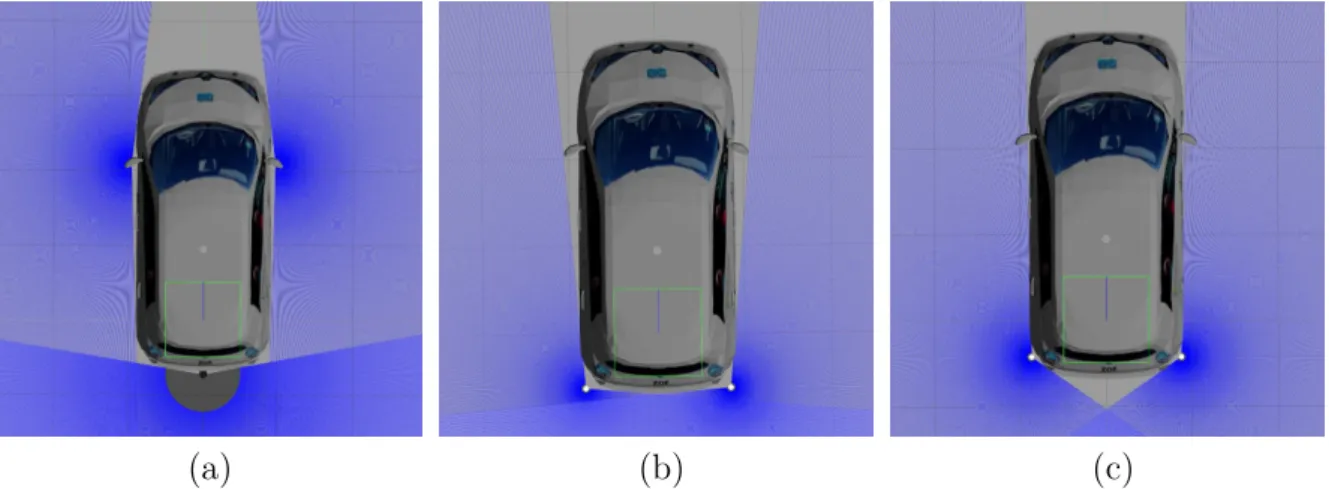
Nevertheless, from the sensors’ placement one can quickly tell that there non-negligible blindspots with the considered perception system. The LMS151 can only perceive on the rear of the vehicle while the perception cone of the VLP-16 doesn’t allow it to detect relatively low nearby obstacles (Fig. 2.3) particularly on the sides and on the rear.

In fact, if a car is placed close to the side, the VLP-16 would not able to detect the closest portions of it as shown in Fig. 2.4. In order to ensure a proper detection, the distance between the cars would have to be increased as shown in Fig. 2.5.

To try to eliminate the previously mentioned blindspot, one could consider adding some low-cost sensors LiDARs as shown in Fig. 2.6. In the configuration proposed in Fig. 2.6a the additional sensors would be placed below the side mirrors while keeping the LMS151 for perception on the rear. The configurations shown in Figs. 2.6b and 2.6c would not require keeping the LMS151 since the perception on the rear would be already covered. The second configuration would provide the best coverage on the rear with a

(a) (b)

Figure 2.3: Perception cone of the VLP-16 placed on top of the vehicle: (a) front and (b) side views.

Figure 2.4: Vehicle to detect placed at a distance of 2.2 m (center to center)

Figure 2.5: Vehicle to detect placed at a distance of 3.35 m (center to center) very good one on the sides but having the drawback of the sensors being relatively far from the vehicle’s body. In the third configuration the sensors would be very close to the body of the vehicle at the expense of a slightly worse perception on the rear, although

(a) (b) (c)

Figure 2.6: Perception capabilities of different sensor configurations (perception cone of VLP-16 omitted for the sake of clarity)

comparable to the one with a single LMS151 on the rear.

Nevertheless, due to different technical and practical reasons, no additional LiDARs where installed in the vehicle.

2.3.2

Sensory data processing

For safety reasons, the perception focuses on the detection of parked cars, which can be approximated by boxes considering that, when viewed from the top, they have a rectangular-like shape.

It should be noted that, since the focus of the work was on the control rather than on the perception problem, the algorithm presented in this section is meant to be considered as an example of how one could perform an online extraction of the required sensor features rather than the only way to do it (e.g [69]). For example, if only one car (or none) was already parked, one could instead use the markings on the ground perceived by a vision system. If a precise enough map and localization system are available, another option would be to generate virtual sensory data from the relative pose between the vehicle and the known parking spots. Finally, one could use a combination of different sensor sources to get a more robust estimation of the parking spot and surrounding obstacles.

Because the two considered sensors provide information of a very similar nature, the data can be fused by simply storing the data provided by the LMS151 as a point cloud and then transforming the point cloud from LMS151’s frame to the VLP-16’s frame so it can be added to the point cloud provided by the latter sensor. For this, it is assumed that

the time difference between the data provided by each sensor is reasonably small, i.e. the data are sufficiently synchronized.

The complete point cloud obtained from the two sensors is first filtered with a couple of crop boxes. The first crop box keeps only the data that are close enough to the car to be relevant in a parking application and that does not represent the floor and afterwards and the second one is used to filter out the points that belong to the car’s body (self-collision sensor readings). Then, an Euclidean Cluster Extraction algorithm is used to have each obstacle represented as a cluster. The orientation of each cluster is extracted by fitting a line model to the points belonging to the contour of the cluster using a RANSAC algorithm. The orientation of the bounding box is equal to the orientation of the fitted line. Then, the rotated bounding box of the cluster is computed using the previously found orientation. We have found from experience that this method gives better results than the one included (getOBB) in the Point Cloud Library (PCL) [75] which is based on the eigenvectors of the cluster.

2.3.3

Parking spot extraction

The (sufficiently large) free space between two parked vehicles is considered as a parking spot. The parked vehicles are represented by red rectangles while the parking spot is represented by a green one in Fig. 2.7.

spot width

d

d

d

/2

d

/2

spot length

c

_c

c

c

c

c

c

c

l

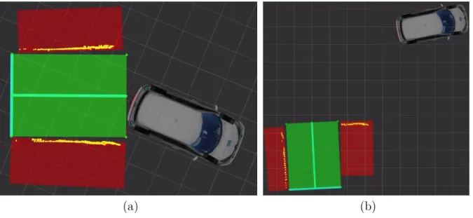
(a) (b)

Figure 2.8: Parking spot extraction from real data: (a) Already parked vehicles not per-fectly aligned, (b) the parked vehicles are not completely visible

First of all, it is necessary to find the two minimum distances between the points defined by the corners of the obstacles with the constraint that the four points that define the two distances have to be different. In Fig. 2.7 the two minimum distances are d1,

defined by c12 and c23, and d2, defined by c11 and c24.

Then, one can find the midpoints between the points that define the aforementioned minimum distances and, with these two midpoints, it’s possible to construct a line ls. One

can extract the parking spot width by adding up the two minimum distances between the line ls and the points that define d1 and d2, with one point of these new distances

on each side of the line ls. To extract the spot length, one can project the points that

define d1 and d2 onto ls and then look for the largest distance among this four projected

points. The center of the parking spot is located along the line ls and at the mid-distance

between the two projected points used to define the parking spot length.

Following this approach, the estimated parking spot adapts automatically in size and orientation to the free space between the two cars even when they are not perfectly parked (Fig. 2.8a) and/or one of them is not completely visible (Fig. 2.8b).

2.3.4

Use of virtual sensors

Assuming that the sensory data can be consistently transformed from a given frame to another, it is possible to use virtual sensors placed at will. The relevant sensors features

are thus transformed and expressed in the most convenient coordinate frame, simplifying the sensor features definitions and their interaction matrices and leading to a generic formulation.

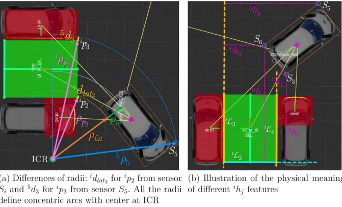
The usefulness of virtual sensors can be exemplified as follows: if the car is parking into a perpendicular spot with a backward motion (Fig. 2.8a), the risk of collision with the obstacle on the left is the highest for the car’s rear left corner, therefore it would be convenient to have a virtual sensor (S6) placed on said corner to measure directly the

distance to the line that defines the left boundary of the parking spot. Indeed, thanks to the use of virtual sensors, different physical sensors may be used as long as the necessary sensor features can be computed.

The virtual sensor placement can be seen in Fig. 2.9. The placement of S1 and S2

correspond, respectively, to the VLP-16 and LMS151. S3 to S6 are placed on the corners

of the car’s bounding rectangle (taking into account the side mirrors) with the purpose of collision avoidance with surrounding obstacles. S7 and S8 are used to prevent hitting

the curb on parallel parking maneuvers thus are placed on the right side corners (with respect to the vehicle) of the dashed orange rectangle whose width and length are equal to wb and lrw+ lfw respectively. S3 to S8 have the same orientation as Fm. All the virtual

sensors are fed using the data extracted from the free parking spot.

Figure 2.9: General sensors’ configuration

2.3.5

Line parametrization

Given two distinct 3D pointsi_p

f andipgexpressed in frame Fiof sensor Siin homogeneous

coordinates, with

i_p

Figure 2.10: Geometric interpretation of a line’s normalized Plücker coordinates

i_p

g = [iXg;iYg;iZg;iWg], (2.11b)

a line passing through them (expressed in the same frame Fi) can be represented using

normalized Plücker coordinates as a couple of 3-vectors [76]:

i_L

j = [iuj;ihj] (2.12)

where i_u

j = iuj/||iuj|| (with iuj 6= 0) describes the orientation of the line and ihj = i_r

j/||iuj|| where irj encodes the position of the line in space. Additionally, it can be

seen (Fig. 2.10) that i_h

j is orthogonal to the plane containing the line and the origin

(interpretation plane). The two 3-vectors i_u

j and irj are defined as [77]: i_u

j =iWf[iXg;iYg;iZg] −iWg[iXf;iYf;iZf] (2.13a) i_r

j = [iXf;iYf;iZf] × [iXg;iYg;iZg] (2.13b)

Due to the planar world assumption considered, the third element ofi_u

j and the first

and second elements of i_h

j are equal to zero, i.e. iuj,3 = ihj,1 = ihj,2 = 0 while, for the

same reason, i_h

j,3 can be interpreted as the signed distance from the origin to the line.

Considering this and for the sake of clarity, for the remaining of the dissertation it would be deemed i_h

j ≡ihj,3. As such, the sensor signal si,j and interaction matrix ˇLi_Lj for the

line i_L

j observed by Si are defined respectively as:

si,j = h_i

u_j,1;iu_j,2;ihj i