Impacts of climate changes on dissolved oxygen
concentrations in Quebec Province lakes
par
Claude Bélanger
1, Raoul-Marie Couture
2, Yves Gratton
1, Isabelle Laurion
1,
Travis Logan
3, Milla Rautio
4and André St-Hilaire
1Août 2017
1 Institut national de la recherche scientifique, Centre eau, terre et environnement, Québec, Qc, Canada
2
NIVA : Catchment Processes Section, Norwegian Institute for Water Research, Oslo, Norvège
3 Ouranos, Montréal, Qc, Canada 4
UQAC : Département des sciences fondamentales, Université du Québec à Chicoutimi, Saguenay, Qc, Canada
ii
Correct citation for this publication:
Bélanger, C., R.-M. Couture, Y. Gratton, I. Laurion, T. Logan, M. Rautio and A. St-Hilaire, 2017. Impacts of climate changes on dissolved oxygen concentrations in Québec Province lakes. Report No R1752, INRS-ETE, Québec (QC): viii + 48 p.
© 2017, Institut national de la recherche scientifique (INRS)
iii
Résumé
L’étendue et la localisation des habitats de plusieurs espèces de salmonidés sont régies par la température de l’eau et les concentrations en oxygène dissous. Le touladi, par exemple, préfère des températures sous les 12° ou 15° C et des concentrations en oxygène dissous supérieures à 4 ou 6 mg L-1. Les gestionnaires qui désirent améliorer la gestion de ces espèces ont besoin d’une meilleure compréhension de l’impact des changements climatiques sur les températures et les concentrations en oxygène dissous dans ces habitats. Notre projet utilise un modèle de lac simple, MyLake, pour reproduire les conditions actuelles de température et d’oxygène dissous dans les lacs et, par la suite, pour proposer des scénarios crédibles de l’évolution de ces habitats dans un futur rapproché (2041-2070) et dans un futur plus éloigné (2071-2100). Afin d’étudier les variations latitudinales entre le Québec et le Nunavik, nous avons produit une section nord-sud (48° à 60° N) des valeurs estimées de la température de l’eau et des concentrations en oxygène dissous pour les deux horizons futurs.
Abstract
The size and location of many salmonid habitats are controlled by water temperature and dissolved oxygen concentrations. Lake trout, for example, prefers water temperatures below 12° to 15 °C and oxygen levels above 4 to 6 mg L-1. To improve the management of these resources, we need a better understanding of how the temperature and oxygen habitats of salmonids will be impacted by expected climate changes. This project used a simple lake model, MyLake, to firstly reproduce current temperature and dissolved oxygen habitats and secondly, to generate plausible habitat scenarios in the near (2041-2070) and more distant (2071-2100) future. Finally, we produced a south-north section of predicted temperature and dissolved oxygen between 48°N and 60°N in the near and far futures to study the latitudinal changes over Nunavik and southern Quebec.
iv
Acknowlegments
We would like to thank Guillaume Grosbois of the Université du Québec à Chicoutimi (UQAC) for extracting and sending us the Simoncouche data. The local meteorological data were sent to us by François Gionet and Prof. Hubert Morin, both also at UQAC. We are also grateful to Prof. Paul del Giorgio of UQAM for the authorisation to use his buoy data. The Lac-du-camp moorings were deployed and recuperated by of a team of technicians from Centre d’Études Nordiques (CEN), including Denis Sarrazin. The temperature data (not used in this report) are under the responsibility of Prof. Reinhard Pienitz and were processed by Denis Sarrazin. The moorings from Lake Jacques-Cartier were deployed and recuperated by Jean-Nicolas Bujold and a team of technicians from the Ministère des Forêts, de la Faune et des Parcs. Thank you very much to everybody.
We would like to thank the MyLake model developers, especially Dr. Tuomo Saloranta, for the authorisation to use MyLake. Configuration of the genetic optimization script was done by Dr. Magnus Norling at the Norwegian Institute of Water Research..
This project was financed by a grant from Ouranos and grants from the National Sciences and Engineering Council of Canada (Discovery program) to Isabelle Laurion and Yves Gratton, as well as by a contract from the Ministère des Forêts, de la Faune et des Parcs.
v
Table of Contents
Résumé ... iii
Abstract ... iii
Acknowlegments ... iv
Table of Contents ... v
List of Tables ... vi
List of figures ... vii
1.
Introduction ... 1
2.
Objectives... 2
3.
Context ... 3
4.
Data and Methods ... 5
4.1 MyLake ... 5
4.2 Data ... 6
4.2.1 Lake Jacques-Cartier data ... 7
4.2.2 Lake Lac-du-camp data ... 7
4.2.2 Lake Simoncouche data ... 11
4.3 MyLake Calibration ... 16
4.3.1 Water Temperature Calibration ... 16
4.3.2 Parameter Selection ... 16
4.3.3 Future horizons (2041-2070 and 2071-2100) simulations ... 19
4.3.4 Selection of a South-North Section... 20
5.
Results ... 21
5.1 Water Temperature Simulations ... 21
5.2 Dissolved Oxygen Simulations ... 21
5.3 Latitudinal Variations ... 24
6.
Summary and Conclusions... 30
7.
Suggested Future Work ... 31
8.
References ... 32
Appendices... 35
Appendix 1 : MyLake possible input and initial variables ... 35
vi
List of Tables
Tableau 1. Characteristics of our three test lakes. “N.A.” stands for data not available. The “Dates sampled” (line 9) are the dates when the temperature (line 10) and dissolved oxygen (line 11) were sampled, unless otherwise specified. ... 8 Tableau 2. Simoncouche Lake: A comparison of temperatures observed through moored
vii
List of figures
Figure 1. Fish habitats. A lake can provide a) a complete habitat, b) a thermal and/or oxygen refuge, or c) no habitat at all. ... 3 Figure 2. Location of lakes Jacques-Cartier (JAC), Chibougamau (CHI), Bédard (BED) and Stewart (STW). The blue squares show the locations of eight hypothetical lakes along the meridian 071 °W (HL1 to HL8). The hypothetical lakes are at the centre of 100 km x 100 km areas and the North American Regional Reanalysis (see section 4.2.2) data at the grid points (red dots) in each area were averaged... 5 Figure 3. Location of lakes Simoncouche, Char and Lac-du-Camp. The purple line shows the location of the original south-north section. The figure is modified after the map of the four ArcticNet IRIS regions from Stern and Gaden (2015). ... 6 Figure 4. Raw dissolved oxygen observations in Lake Jacques-Cartier in 2015-2016. ... 9 Figure 5. Raw dissolved oxygen observations in Lake Lac-du-camp in 2015-2016. ... 10 Figure 6. Left panel: Simoncouche Lake in UQAC's Forêt d'enseignement et de recherche
Simoncouche (FERS). Right panel: Simoncouche depth contours. The Simoncouche River is located at the top of both panels. The Des Îlets outlet may be seen at the bottom of the right panel. ... 11 Figure 7. Simoncouche River outflow into Simoncouche Lake. ... 12 Figure 8. Comparisons between Simoncouche meteorological observations (red), Bagotville observations (blue) and NARR data for global radiation (upper panel), relative humidity (middle panel) and wind speed (lower panel). ... 13 Figure 9. Comparisons between Simoncouche meteorological observations (red) and Bagotville observations (blue) for air temperature (upper panel), relative humidity (middle panel) and wind speed (lower panel)... 13 Figure 10. Temperature at 3 (light blue) and 5 (dark blue) m in lake Simoncouche between 2011 and 2014. The red dashed line is the 4° C theoretical temperature in winter. ... 14 Figure 11. Dissolved Oxygen (DO): vertical profiles between May 2011 and August 2012. ... 15 Figure 12. Dissolved Organic Carbon (DOC) at 3 m (red dots) and 5 m (blue dots) between March 2011 and February 2015... 15 Figure 13. Observed (black) and modeled (blue) water temperature at 3 m (upper panel) and 5 m (lower panel). The depths of the modeled temperature are 1.5 and 5.5 m... 17 Figure 14. Observed (black) and modeled (blue) water temperature at 3 m (upper panel) and 5 m (lower panel). The depths of the modeled temperature are 2.5 and 5.5 m... 17
viii
Figure 15. Locations (marked by four Xs) of the four latitudes along 071° W used for our South-North section. This map shows the number of days with an ice cover for the 1981-2010 climatological period. It was obtained by moving Lake Simoncouche at 1161 locations (the rectangles) over Quebec, Nunavik and Nunatsiavut. ... 20 Figure 16. Dissolved oxygen simulation (blue lines) between 12 May 2011 and 01 November 2012. The red + are the observations. This is the optimized solution: the fraction of incoming DOC available for transformation is 13.70% and kBOD = 0.3410 d-1. ... 22
Figure 17. Dissolved oxygen simulation (blue lines) between 12 May 2011 and 01 November 2014. The red + are the observations. The model was run using the sediment module instead of the SOD formulation; the fraction of incoming DOC available for transformation is 13.70% and kBOD = 0.3410 d-1. ... 22
Figure 18. Observed (red) versus modeled (blue) vertical DO profiles between 12 May 2011 and 21 August 2012. The information is the same as in Figures 16, but it is presented differently. ... 23 Figure 19. Influence of the latitudinal gradient for Simoncouche Lake, for the period 1981-2010. The Figure presents the results at four latitudes: 48.25° (red), 51.25° (orange), 55.75° (green) and 59.25° (blue). The ticks on the x axis indicate the months of the year (dd/mm). ... 25 Figure 20. Influence of the latitudinal gradient for Simoncouche Lake, for the period 2041-2070. The Figure presents the results at four latitudes: 48.25° (red), 51.25° (orange), 55.75° (green) and 59.25° (blue). The ticks on the x axis indicate the months of the year (dd/mm). ... 26 Figure 21. Influence of the latitudinal gradient, for Simoncouche Lake, for the period 2071-2100. The figure presents the results at four latitudes: 48.25° (red), 51.25° (orange), 55.75° (green) and 59.25° (blue). The ticks on the x axis indicate the months of the year (dd/mm). ... 27 Figure 22. Impacts of climate changes on dissolved oxygen distribution. The figure presents the differences between the period 2041-2070 with respect to the reference period 1981-2010. The figure present the differences at four latitudes: 48.25° (red), 51.25° (orange), 55.75° (green) and 59.25° (blue). The ticks on the x axis indicate the months of the year (dd/mm). ... 28 Figure 23. Impacts of climate changes on dissolved oxygen distribution: differences between the period 2071-2100 with respect to the reference period 1981-2010. The figure present the differences at four latitudes: 48.25° (red), 51.25° (orange), 55.75° (green) and 59.25° (blue). The ticks on the x axis indicate the months of the year (dd/mm). ... 29
1
1. Introduction
This report is the fourth report produced for Ouranos and the Ministère des Forêts, de la Faune et des Parcs between November 2015 and August 2017. The four reports are
Influence de la profondeur moyenne d’un lac sur la température de l’eau et variations latitudinales : Une étude de sensibilité menée à l’aide du modèle unidimensionnel MyLake (Bélanger et al., 2016).
Analyse multivariée des paramètres morphologiques des lacs de la province de Québec
(Chimi Chiadjeu et al., 2016).
Cartographie des variations spatiales et futures de la disponibilité des habitats thermiques favorables aux salmonidés dans les lacs du Québec : méthodologie et exemples (Bélanger et al., 2017).
Impacts of climate changes on dissolved oxygen concentrations in Québec Province lakes (Bélanger et al., 2017; this report).
This work was originally suggested by fish ecology biologists of the Ministère des Forêts, de la Faune et des Parcs du Québec. They were looking for tools to better manage the recreational and subsistence fisheries in northern Quebec. Due to their preference for cold-water conditions, climate warming may potentially affect the habitats of all salmonids living in northern Quebec, Nunavik and Nunavut lakes, including species important for subsistence fishery such as Lake trout and Arctic char. The size and location of the habitats of those species are governed by the seasonal temperature and dissolved oxygen distributions. Phase 1 of this project was dedicated to adapt the Norwegian Institute for Water Research MyLake model to describe fish thermal habitats in the province of Québec (Bélanger et al., 2013). Phase II addresses the four questions behind the four studies listed above. This report describes only our efforts to adapt a version of MyLake that handles dissolved oxygen (Couture et al., 2015) to Quebec Province lakes.
After briefly presenting the objectives (Chapter 2), we will review the problem (Chapter 3) and present the model and the data (Chapter 4). Preliminary results will be presented in Chapter 5, followed by a Summary and Conclusions (Chapter 6) and a list of suggested future work (Chapter 7).
2
2. Objectives
The principal objective of the overall project is to produce better tools for fishery managers in Quebec, Nunavik and Nunavut. We will attain this objective through the following two specific objectives.
The first specific objective is to produce maps of the forecasted scenarios of changes in ice cover and fish thermal habitats, which are also a function of the local physical, chemical and topographic conditions.
Another specific objective is to reproduce the dissolved oxygen local distributions in selected lakes, to produce scenarios of potential oxygen variations for typical lakes and drainage basin configurations for the horizon 2041-2070 and 2071-2100.
3
3. Context
Climate changes are already affecting fish communities of northern lakes directly through the change in water temperature. Cold stenothermal fauna sensitive to even small changes in water temperature appears naturally more at risk. In addition to thermal stress, increased parasitism and competition could also contribute to the decline of these endemic species (Vincent at al., 2011). The changes in temperature, light and nutrients availability may also have a qualitative effect on species composition and diversity at the primary producer level (Peeters et al. 2007, Thackeray et al. 2008). An often-mentioned concern regarding this possibility is a shift toward dominance by species of cyanobacteria that form noxious bloom (Paerl & Huisman 2008). The overarching goal of the proposed project is to ensure the perenniality of the salmonid subsistence fisheries in northern lakes, such as Lake trout (Salvelinus namaycush) and Arctic char (Salvelinus alpinus), and the conservation of fish stocks for future generations. To attain that goal, we need a better understanding of the transformations of the lentic salmonid habitats, as defined by the spatial and the temporal variations of the extent of appropriate temperature-oxygen conditions for these fishes. All fish species have a preferred temperature range and a minimum oxygen level necessary for their survival. Lake trouts, for example, prefer water temperatures below 12° or 15 °C, depending on the authors, and oxygen levels (DO) above 4 or 6 mg L-1 (Plumb and Blanchfield, 2009). Some lakes can provide a suitable
habitat all year round for a given species, while in other cases, only a small part of the lake is suitable during some period of the year, in summer for instance; these reduced habitats are called “refuges” (Fig. 1). In some
cases, the preferred habitats can even disappear during part of the year. We propose to estimate possible changes in water temperature, ice cover duration,
and content in dissolved oxygen for some lakes of Nunavut, Nunatsiavut, Nunavik and northern Quebec for the horizons 2041-2070 and 2071-2100. A shift in the spatial distribution of many species can then be forecasted, some species being driven to extinction in some lakes while other species would be able to colonise the new warmer habitats. The possible displacement of native fishes in northern lakes is of particular concern to Inuit and First Nations communities. The practical applications of our expected results will be to improve tools for the managers of this important subsistence resource to help them optimize their fish population protection efforts and minimize the costs associated with securing the long-term perenniality of these species. The habitat mapping that we will produce, combined with fish population data acquired by the managers (MFFP and Makivik), will be used to map current and future fish productivity indexes and, in turn, help them decide on fish population management and habitat protection measures.
Figure 1. Fish habitats. A lake can provide a) a complete habitat, b) a thermal and/or oxygen refuge, or c) no habitat at all.
4
Greenhouse gases accumulate in the atmosphere as a result of human activities. Taking into account likely future concentrations, global climate models predict an increase in air temperature of several degrees by the end of the twenty-first century and large changes in the regional distribution and intensity of precipitations (IPCC, 2013). These shifts in climate have already begun and are expected to modify the physical, chemical and biological attributes of lake water masses and affect their ability to maintain the present-day communities of aquatic plants, animals and microbes (Vincent, 2009). The possibility of significant change to many of the present lake ecosystems appears even more likely when considering that the majority of the world’s lakes are located between latitudes of about 47° and 73 °N (Global Lakes and Wetland Database; Lehner and Döll, 2004), where warming is expected to be more pronounced (UNEP, 2012). Climate changes may affect directly the physical, chemical and biological characteristics of lakes, and also indirectly through modifications in the surrounding watershed. For dimictic boreal lakes, that is lakes that mix completely from surface to bottom twice a year, the most evident impacts include increased durations of ice-free conditions, increase in water column temperature and stronger stratification (vertical density structure) in summer. Larger future differences between air and surface water temperatures result in larger sensible heat transfer (conduction), and an earlier loss of snow and ice cover means a longer period of sensible heat transfer. Similarly, a shorter period of ice cover is expected to change the underwater irradiance regime and result in increased solar energy penetrating the water column. Both conductive and radiative effects lead to warmer surface waters in summer and stronger stratification which tends to lower downward transport of heat via turbulent mixing. One of the potential effects will be to modify fish habitats and their refuges. The shorter duration of the ice cover may also impact other aspects of the irradiance regime and lead to an increased availability of photosynthetically available radiation (PAR) for primary production as well as an increased exposure to ultraviolet radiation. All these physical changes (ice cover, temperature, stratification and mixing) may affect vertical gradients in lake properties and lead to significant effects on phytoplankton production and availability of food for higher trophic levels.
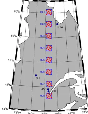
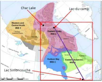
In a previous study (Bélanger et al. 2013), we showed that the MyLake MyLake model (Saloranta and Andersen, 2007) could reproduce the thermal habitats and salmonid thermal refuges in lakes located in the province of Quebec. We also discussed the impacts of climate changes not only on thermal habitats but also on ice cover at eight locations along a north-south gradient between 45°N and 60°N (see Fig. 2). The other limiting condition for fish survival is the dissolved oxygen levels in lakes. The development of a tool that can provide insight on potential impacts of climate changes on these oxygen levels is feasible, given that Couture et al. (2015) have already added an oxygen module and a sediment module to MyLake. An oxygen advection-diffusion model is a model based on the mass conservation equation for oxygen: local-time-variation + advection + diffusion = sources – sinks. The critical step in this approach consists in defining the sources and the sinks correctly. The sinks are water column and benthic respirations. The sources are photosynthesis, inflowing oxygenated river water and exchanges with the atmosphere. We need oxygen and oxygen-related observations to calibrate this new component of the model. This means that we need to revisit our target lakes to obtain simultaneous time series of dissolved oxygen and temperature, as well as meteorological inputs, dissolved organic matter (DOC) and other biological variables (see the methodology section). Originally, we proposed to extend our study to Nunatsiavut and Nunavut to represent a wider gradient of physical conditions (Fig. 3). Unfortunately, we had to limit the study to northern Quebec and Nunavik, because of time constraints.
5
4. Data and Methods
4.1 MyLake
We are using the one-dimensional (1-D) MyLake model (Multi-Year Lake model) developed at the Norwegian Institute for Water Research (NIVA) (Saloranta and Andersen, 2007). In addition to simulating the evolution of temperature over the entire water column, MyLake also simulates the evolution of ice and snow covers. The model time step is 24 h and the required inputs are lake bathymetry (expressed as the area per meter of depth in our version), initial thermal conditions and time series of daily values for seven meteorological variables, namely air temperature, relative humidity,
atmospheric pressure, wind speed, precipitations, global radiation, and cloud cover. The model was modified and tested in Phase 1 for four lakes (see Fig. 2): Bédard (BED: 47.27°N, 71.12°W), Jacques-Cartier (JAC: 47.58°N and 71.22°W), Chibougamau (CHI: 49.83°N, 74.28°W) and Stewart (STW: 58.19°N, 68.43°W) using water temperature and local meteorological observations. The temperature simulations were in surprisingly good agree-ment with observations in all cases (Bélanger et al. 2013). MyLake will be used to estimate past and future climatological annual cycles (in the sense of 30-year climatology) of water temperature in selected lakes: a small southern lake, Simoncouche (SIM; Fig. 3), a small northern lake, Lac-du-camp (LAC; Fig. 3), a medium lake, Stewart (STW; Fig. 2), and a large lake, Jacques-Cartier (JAC; Fig. 2). Changes in DO concentrations in a lake result from the exchange of oxygen at the air-water interface, at the water-bottom interface, and as a response to the balance between photosynthetic production and respiratory consumption. The physical flux at the air-water interface is calculated from the difference between DO concentrations and the saturation value (the concentration for
which there is equilibrium with the atmosphere at ambient temperature). This flux will be affected by the piston velocity effect of the wind speed. Couture et al. (2015) have already added an oxygen module and a sediment module to MyLake. They added physical exchanges of DO between air and water to the model based on Staehr et al. (2010). The biochemical drivers of oxygen dynamics added to MyLake are phytoplankton biomass and dissolved organic matter (DOC), both native MyLake state variables. Permafrost degradation will also have a geographical impact on DOC concentrations (Frey and McClelland 2009) and should be taken it into account
78o W 75oW 72oW 69oW 66oW 63oW 44oN 48oN 52o N 56oN 60oN HL1 HL2 HL3 HL4 HL5 HL6 HL7 HL8 STW CHI JAC BED
Figure 2. Location of lakes Jacques-Cartier (JAC), Chibougamau (CHI), Bédard (BED) and Stewart (STW). The blue squares show the locations of eight hypothetical lakes along the meridian 071 °W (HL1 to HL8). The hypothetical lakes are at the centre of 100 km x 100 km areas and the North American Regional Reanalysis (see section 4.2.2) data at the grid points (red dots) in each area were averaged.
6
in northern regions. All the parameters that can be handled by MyLake are listed in Appendix 1. However, we will begin, as in Staehr et al. (2010), by using a simple benthic respiration. This can only be done if we measure all the other parameters necessary to test our parameterization. Modeling the contribution of DOC, for instance, is based on inflows, biodegradation and photochemical UV oxidation.
Figure 3. Location of lakes Simoncouche, Char and Lac-du-Camp. The purple line shows the location of the original south-north section. The figure is modified after the map of the four ArcticNet IRIS regions from Stern and Gaden (2015).
A module simulating the bacterial decay of DOC has recently been added to MyLake (Holmberg et al., 2014) to look at the effects of climate changes on boreal lakes DOC. The last parameter is the benthic respiration. MyLake also includes a water-sediments interaction module. A simplified first step will be to set a bottom respiration boundary condition as a Sediment Oxygen Demand (SOD) according to Walker and Snodgrass (1986). The last step is to run a genetic algorithm to optimize the relevant model parameters (Deb 2000, cited in the Matlab Global Optimization Toolbox, v. 2017a).
4.2 Data
As mentioned earlier, we needed to sample our targeted lakes concurrently for temperature (every other meter, if possible), dissolved oxygen (1 m from the surface and one meter from the bottom), and DOC (at least one value). Lake Jacques-Cartier was sampled in 2015-2016 for temperature (TidbiT loggers) and dissolved oxygen (MiniDOT loggers) by the MFFP (Jean-Nicolas Bujold). INRS-ETE (Isabelle Laurion) sampled Lac-du-camp for temperature (Vemco minilogs) and dissolved oxygen (MiniDOT loggers) in 2015-2016. Lake Stewart was not sampled in 2015-2016 because of time and budget constraints. The last two lakes, Char (in Nunavut) and Simoncouche (in southern Quebec), were also chosen because of their existing
7
exhaustive, multi-disciplinary data base. Char Lake was kept “in reserve” and Simoncouche Lake was selected to calibrate MyLake because it was sampled by GRIL (Groupe de recherche interuniversitaire en limnologie et en environnement aquatique; Milla Rautio and Paul del Giorgio) between 2011 and 2015. A subset of the available data is presented in Table 1. We will very briefly present the dissolved oxygen observations for lakes Jacques-Cartier and Lac-du-camp as they were sampled for this project. This will be followed by a detailed description of the observations from lake Simoncouche.
4.2.1 Lake Jacques-Cartier data
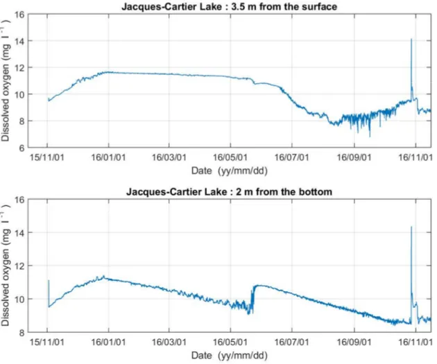
The 2015-2016 dissolved oxygen observations (DO) are presented in Figure 4. The signal is quite clear, even if these are the raw, unprocessed data. There is a possible inaccuracy of 1 m in the actual depths of the sensors: a quality control operation is needed. The surface and bottom concentrations were the lowest in late September, increasing steadily until ice formation in late December. The lowest temperature observed at 3.5 m was 0.79° C on December 22. On March 23rd, the ice thickness was still 71.4 cm, on average (68.5, 72.5, 73.5, 73.0, 69.5, 71.0 and 72.0 cm). Near the surface, the DO decreased very slowly until the ice disappeared. Near the bottom (at a depth of 46 m), the winter decrease was more pronounced: the lowest concentrations were found around May 15 (9.30 mg L-1). Surprisingly, the concentrations increased to over 10.80 mg L-1 over the next 15 days, to decrease again until the end of October. No DOC observations were found in the MFFP lake data base.
4.2.2 Lake Lac-du-camp data
The 2015-2016 dissolved oxygen observations (DO) are presented in Figure 5. The signal is also quite clear, even if these are the raw, unprocessed data. The concentrations near the surface begin to change abruptly on 4 August 2011 (19h00, UTC). This decrease (14.83 to 10.89 mg L-1) lasted approximately 36 hours until 10h00 on 6 August. The decrease came with an increase of almost 2° C in water temperatures (9.1°C to 10.8°C; not shown). The saturation percentage decreased from 128% to 98%. The saturation concentration of oxygen at 10.8° C is 11.1 mg L-1. This could explain the rapid decrease in concentration. The bottom concentrations reached their maximum (13.34 mg L-1) on October 2nd and were for all purposes equal to the surface concentrations. The concentrations decreased slowly until 10 June 2012 when they increased abruptly over a four day period.
8
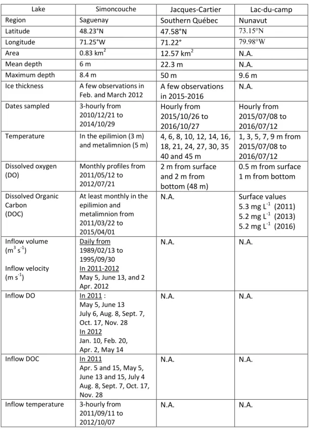
Tableau 1. Characteristics of our three test lakes. “N.A.” stands for data not available. The “Dates sampled” (line 9) are the dates when the temperature (line 10) and dissolved oxygen (line 11) were sampled, unless otherwise specified.
Lake Simoncouche Jacques-Cartier Lac-du-camp Region Saguenay Southern Québec Nunavut
Latitude 48.23°N 47.58°N 73.15°N
Longitude 71.25°W 71.22° 79.98°W
Area 0.83 km2 12.57 km2 N.A.
Mean depth 6 m 22.3 m N.A.
Maximum depth 8.4 m 50 m 9.6 m
Ice thickness A few observations in Feb. and March 2012
A few observations in 2015-2016
N.A. Dates sampled 3-hourly from
2010/12/21 to 2014/10/29 Hourly from 2015/10/26 to 2016/10/27 Hourly from 2015/07/08 to 2016/07/12 Temperature In the epilimion (3 m)
and metalimnion (5 m) 4, 6, 8, 10, 12, 14, 16, 18, 21, 24, 27, 30, 35 40 and 45 m 1, 3, 5, 7, 9 m from 2015/07/08 to 2016/07/12 Dissolved oxygen (DO)
Monthly profiles from 2011/05/12 to 2012/07/21 2 m from surface and 2 m from bottom (48 m) 0.5 m from surface 1 m from bottom Dissolved Organic Carbon (DOC)
At least monthly in the epilimion and
metalimnion from 2011/03/22 to 2015/04/01
N.A. Surface values 5.3 mg L-1 (2011) 5.2 mg L-1 (2013) 5.2 mg L-1 (2016) Inflow volume (m3 s-1) Inflow velocity (m s-1) Daily from 1989/02/13 to 1995/09/30 In 2011-2012
May 5, June 13, and 2 Apr. 2012
N.A. N.A.
Inflow DO In 2011 : May 5, June 13 July 6, Aug. 8, Sept. 7, Oct. 17, Nov. 28 In 2012 Jan. 10, Feb. 20, Apr. 2, May 14 N.A. N.A. Inflow DOC In 2011
Apr. 5 and 15, May 5, June 13 and 15, July 4 Aug. 8, Sept. 7, Oct. 17, Nov. 28
N.A. N.A.
Inflow temperature 3-hourly from 2011/09/11 to 2012/10/07
9
10
11
4.2.2 Lake Simoncouche data
Lake Simoncouche was selected to calibrate the version of MyLake with dissolved oxygen because of the availability of simultaneous physical, chemical, biological and meteo-rological observations. The lake is located in Université du Québec à Chicoutimi’s « Forêt d’enseignement et de recherche Simoncouche» near Saguenay (Fig. 6) and it is considered as one of the GRIL infrastructures. It is also a member of the GLEON (Global Lake Ecological Observatory Network) lake Network. The lake characteristics and the available data are presented in Table 1. This lake is also convenient because there are two local meteorological stations nearby, including one on the lake’s shores. The Bagotville Airport meteorological station is also only 24 km away. The lack of sediments observations is not critical as we are not planning to use the sediment module in our first simulations. The PPZD module will also be turned off. We will use the inflow data, the temperature data, the dissolved oxygen data and the dissolved organic carbon data for our first model runs.
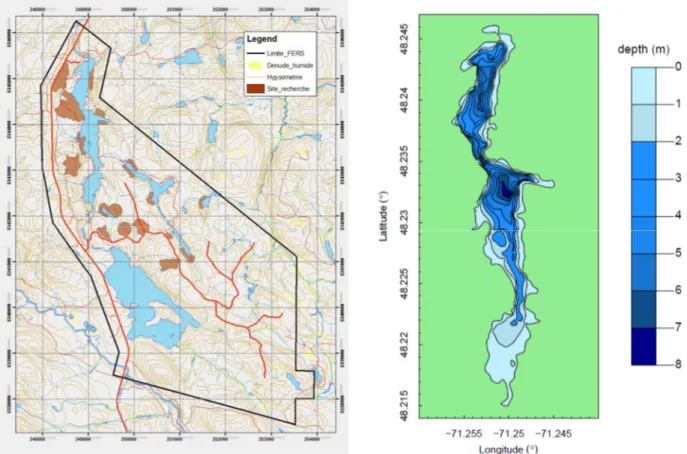
Figure 6. Left panel: Simoncouche Lake in UQAC's Forêt
d'enseignement et de recherche Simoncouche (FERS). Right panel: Simoncouche depth contours. The Simoncouche River is located at the top of both panels. The Des Îlets outlet may be seen at the bottom of the right panel.
Figure 6 presents the location of lake Simoncouche within the “Forêt d’enseignement et de recherche Simoncouche”. The lake is composed of two basins separated by a narrow bottleneck. All the profile data was obtained at the lake deepest point.
12
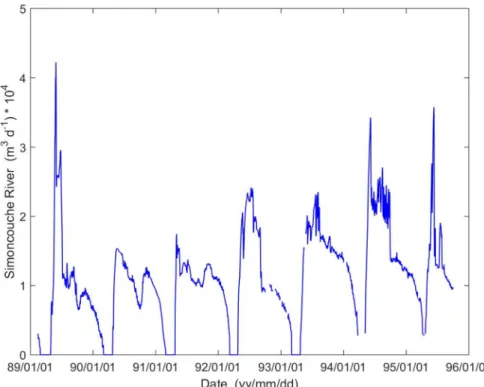
Hydrometric Data.The principal Simoncouche inlet is the Simoncouche River (Fig. 6). River flow data were obtained from the « Ministère du Développement durable, de l'Environnement et de la Lutte contre les changements climatiques » for the period 1989-1995, the only available data set. The data are presented in Fig. 7. The five-year daily observations were simply averaged by day of the year and used as boundary conditions for water inflow.
Figure 7. Simoncouche River outflow into Simoncouche Lake.
Meteorological Data.
The meteorological observations are critical since they will control the water temperature in the lake in the past (simulation period) and also in the future (climatological simulation periods). In the delta method (see section 4.3.3), we are simply adding monthly deltas to local observations for a single lake or to the North American Regional Reanalysis (NARR; Mesinger et al., 2006) data for the future horizons (2041-2070 and 2071-2100). However, we always calibrate MyLake with local observations. We found major differences between the local meteorological observations and both the Bagotville observations and the NARR data. It can be seen from Figures 8 and 9 that the global radiation and the wind speed do not correspond with the other two observation sources, while the observations from Bagotville and NARR are similar. We were unable to find a correction or a conversion factor. Therefore, we used the global radiation from NARR and the wind speed from Bagotville.
13
Figure 8. Comparisons between Simoncouche meteorological observations (red), Bagotville observations (blue) and NARR data for global radiation (upper panel), relative humidity (middle panel) and wind speed (lower panel).
Figure 9. Comparisons between Simoncouche meteorological observations (red) and Bagotville observations (blue) for air temperature (upper panel), relative humidity (middle panel) and wind speed (lower panel).
14
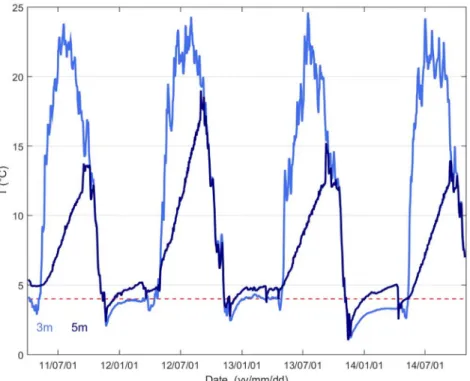
Water Temperature Data.Water temperature was available only at two depths: in the epilimnion and the metalimnion. The nominal depths were 3 and 5 m, respectively (Fig. 10). There seems to be some inconsistencies in the depths of the observations. We will discuss it further in section 4.3 “MyLake Calibration”.
Figure 10. Temperature at 3 (light blue) and 5 (dark blue) m in lake Simoncouche between 2011 and 2014. The red dashed line is the 4° C theoretical temperature in winter.
Dissolved Oxygen (DO) Data
Since vertical oxygen profiles are only available between 12 May 2011 and 28 August 2012, our dissolved oxygen simulation period will run from 12 May 2011 to 01 November 2012. The vertical profiles are shown in Figure 11. The average DO in the incoming water was found to be approximatively 8.0 mg L-1 (average value). This value was used as the daily inflow condition.
Dissolved Organic Carbon (DOC) Data
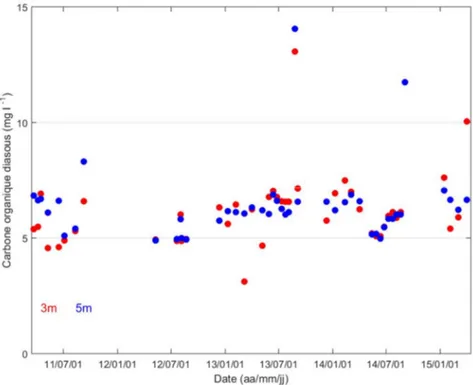
DOC was measured in the epilimnion and the metalimnion approximately once a month between March 2011 and April 2015. The observations are presented in Figure 12. The values are quite constant, if we ignore a few outliers. Samples were also obtained from the Simoncouche River (5.086, 5.524, 4.600, 6.548 mg L-1) between 5 April 2011 and 13 June 2011, and from the lake where the river comes in (6.377, 4.300, 5.600, 6.100, 5.400 and 5.000 mg L-1) from 15 June 2011 to 28 November 2011, for an average value of 5.423 mg L-1. We chose to use the average of the values from the data in Fig. 12, 6.01 mg L-1, as the daily inflow condition.
15
Figure 11. Dissolved Oxygen (DO): vertical profiles between May 2011 and August 2012.
Figure 12. Dissolved Organic Carbon (DOC) at 3 m (red dots) and 5 m (blue dots) between March 2011 and February 2015.
16
Dissolved Inorganic Carbon (DIC) DataA few DIC observations were available (not shown). However, this parameter is ignored for now.
4.3 MyLake Calibration
4.3.1 Water Temperature Calibration
The depths of the temperature data are suggested to be 3 m and 5 m. We believe that there were located around 2.0 or 2.5 m, and around 5.5 m, respectively. The water temperature series come from three mooring deployments: 5 April 2011 to 21 September 2011, 21 September 2011 to 10 October 2012, and from 10 October 2012 to 29 October 2014. The moorings were retrieved and redeployed twice: it is absolutely normal to observe some shift in the data when the depths are not exactly the same. This is what we observe in Figures 10 (observed water temperatures), 13 and 14 (modeled versus observed water temperatures). The difference between Figures 13 and 14 is the simulation depth: 1.5 m in Fig 13 and 2.5 m in Fig. 14. MyLake is a level model: some variables are evaluated at the layer interfaces (0 m, 1 m, etc.) while the state variables (temperature and dissolved oxygen) are evaluated between levels. We observe, in Figure 10, that the temperatures of the hypolimnion are larger in the summer of 2012 than the temperature observed in the other three summers. Moreover, the simulations produce temperatures in the hypolimnion consistent from one year to the other. Therefore, the hypolimnion sensor deployed from 21 September 2011 to 10 October 2012 is not at the same depth than the other three years. We compare, in Table 2, the observations from the moored instruments and the vertical profiler. The depth of the upper instrument seems closer to 2.0 or 2.5 m than to 3 m, while the depth of the lower instrument is always at depths larger than 5 m when compared with the profiler readings. We will use 2.5 and 5.5 as the depths of the instruments and 1.5 m as the simulation depth.
4.3.2 Parameter Selection
All the parameters, reaction equations and module descriptions may be found in Couture et al. (2015) and it supporting information. Information about the temperature model may be found in Saloranta and Andersen (2007). The optimal values of some parameters have been obtained through an optimization process. Other optimization processes could have been used, but we chose to use the genetic algorithm included in the Matlab
Optimization Toolbox v. 2017a (https://www.mathworks.com/discovery/genetic-algorithm.html) (Deb, 2000). The following definition was extracted from this Matlab web site. “A genetic algorithm is a method for solving both constrained and unconstrained optimization problems based on a natural selection process that mimics biological evolution. The algorithm repeatedly modifies a population of individual solutions. At each step, the genetic algorithm randomly selects individuals from the current population and uses them as parents to produce the children for the next generation. Over successive generations, the population "evolves" toward an optimal solution.”
17
Figure 13. Observed (black) and modeled (blue) water temperature at 3 m (upper panel) and 5 m (lower panel). The depths of the modeled temperature are 1.5 and 5.5 m.
Figure 14. Observed (black) and modeled (blue) water temperature at 3 m (upper panel) and 5 m (lower panel). The depths of the modeled temperature are 2.5 and 5.5 m.
18
Tableau 2. Simoncouche Lake: A comparison of temperatures observed through moored instruments (time series) and profiles.
Profile date and time T from Inferred depth T from Inferred depth
upper instrument
of upper instrument lower instrument
of lower instrument
from profile from profile
(°C) (m) (°C) (m) 2011 May 12 08:45 6.276 2.59 4.943 5.81 2011 Jun 15 09:10 17.705 2.00 6.120 > 6 2011 Jul 6 10:00 22.751 2.16 7.754 > 6 2011 Aug 10 08:45 22.044 2.85 10.227 > 6 2011 Sep 8 10:15 17.231 4.12 11.469 > 6 New mooring 2011 Oct 19 10:40 10.699 6.00 10.513 > 6 2011 Dec 4 10:25 2.865 2.41 3.634 4.45 2012 Jan 12 10:10 3.738 1.96 4.529 3.65 2012 Feb 22 09:15 3.887 2.32 4.993 3.59 2012 Mar 28 08:24 3.102 2.00 4.579 5.93 2012 May 16 09:20 13.908 3.08 7.530 > 6 2012 Aug 20 09:45 20.500 4.00 15.797 5.80 2012 Aug 21 N.A. 20.272 3.64 15.835 5.73
19
The variables with the greatest impacts on oxygen concentrations are temperature, ice freeze-up and melt dates and DOC. The saturation concentration of oxygen decreases with higher temperature while early ice-melt dates increase the length of air-water exchange periods. The impact of larger DOC concentrations is to decrease the oxygen concentrations via enhanced microbial metabolism (Couture et al,, 2015), among other effects. One of the most important parameters is the fraction of available incoming DOC, the allochthonous (or refractory) versus the autochthonous (or labile) fraction. The optimization process suggests that only a small fraction (13.70 %) of the incoming DOC should be available for transformation in Simoncouche Lake. This means that labile fraction should also vary with latitude as the DOC of the surface runoff waters will change with the nature of the soils of the drainage basins. The other important parameters highlighted by the optimization process are the daily Biochemical Oxygen Demand (kBOD = 0.3410 d-1) and the Sediment Oxygen Demand (kSOD = 101.6880 mg m-2). The
former is the fraction of oxygen needed to break down organic material in the water column (modeled after Fang and Stefan, 2009) while the latter is the fraction of Biological SOD (BSOB) and chemical SOD (CSOD) needed by the sediments (modeled after Walker and Snodgrass, 1986). Again, Couture et al. (2015) proposed a sediment module based on carbon diagenesis, but we don’t have depth profiles of sediment concentrations necessary to calibrate this module, thus using the robust SOD approach instead. There are other parameters in MyLake, but they appear to be less critical. Nevertheless, a more systematic parameter study is needed. Oxygen sensors (MiniDOTs) were deployed near the surface and near the bottom of lakes Jacques-Cartier and Lac-du-camp to validate the air-water and sediment-water DO exchange parametrizations.
4.3.3 Future horizons (2041-2070 and 2071-2100) simulations
The meteorological data used for future horizons are the NARR data for the reference period (1981-2010) modified according to the delta method (Huard et al., 2014). The NARR model assimilates a great amount of observational data to produce a long-term picture of weather over North America. Deltas are the differences, weekly or monthly, between a simulation for a reference period (1981-2010) and a simulation for a future period (2041-2070 or 2071-2100), for a given numerical climatological model. We used these deltas to project the local meteorological observations in the future by adding the deltas to the “real” meteorological observations at a “real” lake location. To study the impact of climate changes on a typical or hypothetical lake, we begin by simulating the evolution of the lake state variables (temperature and dissolved oxygen) for thirty years using NARR data for the reference period (1981-2010). We then add the deltas for a time period (2041-2070 or 2071-2100) to the NARR reference period data and restart the simulations. Both thirty year series, past and future, are averaged by day of the year and subtracted from each other to obtain the estimated changes. Deltas are either additive or multiplicative, depending on the considered variable. Future data sets are obtained by adding deltas to the reference data (air temperature, solar radiation, pressure, cloud cover) or by multiplying the reference data (wind speed and precipitations) by the deltas. We used the monthly deltas produced by Ouranos (Logan 2016) using a single simulation with the Canadian Regional Climate Model (CRCM5; Martynov et al., 2013). The most pessimistic greenhouse gas emission scenario of the Representative Concentration Pathways (RCP) scenarios is scenario RCP 8.5 (IPCC 2014). This is the scenario that was used to produce the deltas.
20
4.3.4 Selection of a South-North Section
Figure 15. Locations (marked by four Xs) of the four latitudes along 071° W used for our South-North section. This map shows the number of days with an ice cover for the 1981-2010 climatological period. It was obtained by moving Lake Simoncouche at 1161 locations (the rectangles) over Quebec, Nunavik and Nunatsiavut.
As mentioned in the Introduction, we have produced, for the MFFP, 15 different maps (habitat indicators) for each one of our three test lakes (Simoncouche, Stewart and Jacques-Cartier) and for each one of the three climatological periods (1981-2010, 2041-2070 and 2071-2100), for a total of 135 maps. Figure 15 present the number of days with ice cover at the horizon 1981-2010. This map was obtained by running MyLake at 1161 locations using Lake Simoncouche. At each location, the local NARR meteorological data was used, adding orographic and latitudinal effects to the simulations. As time was running short, we selected four locations (instead of eight or ten, as originally proposed) with different ice cover durations (Fig. 15) for our south-north section.
21
5. Results
5.1 Water Temperature Simulations
Water temperature simulations and observations from May 2011 to October 2014 were presented in Figure 13. As mentioned in section 4.2.2, we chose to use the global radiation data from NARR instead of the data from Bagotville. The reason is that the heat transmitted to Lake Simoncouche by the Bagotville data was insufficient to reproduce the heat maximums observed in the lake, even in the first layer (0 to 1 m). The agreement between the observations and the model is quite good, considering that MyLake is a one-dimensional model. The main differences are the following.
Simulated epilimnion temperature are slightly larger than observations in winter; Fall cooling is slightly too early;
Simulated hypolimnion maximum temperatures are slightly lower than the observations.
This could be partly due to the fact that it was difficult to match the depth of the simulations to the depth of the observations. However, the temperature simulations may be considered are “reasonably accurate” and we will ignore these small errors when we will discuss the dissolved oxygen simulations in the next section.
5.2 Dissolved Oxygen Simulations
The dissolved oxygen observations are from vertical profiles: we will assume that the depths of the observations are error-free even if they can vary according to Table 2. To produce model results at similar depths, two layers of dissolved oxygen concentrations are averaged: 0.5 and 1.5 m, 2.5 and 3.5 m, and 4.5 and 5.5 m. The optimal (so far) dissolved oxygen simulation is presented in Figure 16. The model follows the observations until the first winter when the modeled oxygen utilization under the ice is too large near the surface (epilimnion). It appears to recuperate as soon as the ice begins to melt. The model fares very well in the metalimnion over the complete simulation period while the results begin to degrade in the middle of the first winter in the hypolimnion. Clearly, surface and bottom oxygen utilisation need to be improved.
Figure 17 presents a simulation covering the complete water temperature observations period: from May 2011 to October 2014, even if no DO observations are available between May 2012 and October 2014. This simulation uses the sediment module instead of the SOD formulation, and the parameters used for the sediment module are those of Couture et al. (2015). Figure 18 present the same information as in Fig. 16, but in the form of vertical profiles. The differences between the observed and modeled epilimnion and hypolimnion can be seen much more clearly. Three conclusions may be drawn from Figures 16, 17 and 18. Firstly, the model is stable year after year, after a short adjustment period. Secondly, a good set of observations is needed to run the sediment module. Thirdly, a “simple” SOD formulation will be adequate in many situations.
22
Figure 16. Dissolved oxygen simulation (blue lines) between 12 May 2011 and 01 November 2012. The red + are the observations. This is the optimized solution: the fraction of incoming DOC available for transformation is 13.70% and kBOD = 0.3410 d-1.
Figure 17. Dissolved oxygen simulation (blue lines) between 12 May 2011 and 01 November 2014. The red + are the observations. The model was run using the sediment module instead of the SOD formulation; the fraction of incoming DOC available for transformation is 13.70% and kBOD = 0.3410 d-1.
23
Figure 18. Observed (red) versus modeled (blue) vertical DO profiles between 12 May 2011 and 21 August 2012. The information is the same as in Figures 16, but it is presented differently.
24
5.3 Latitudinal Variations
The version of the dissolved oxygen model presented in Figure 16 was run for four latitudes (48.25°, 51.25°, 55.75° and 59.25°; see Fig. 15) and for three simulation periods (1981-2010, 2041-2070 and 2071-2100). The NARR data was used for the 1981-2010 period while the NARR data plus the corresponding deltas was used for the other two periods. The results are presented in Figures 19, 20 and 21. The differences between the periods 2041-2070 and 1981-2010 are presented in Figure 22, while the differences between the periods 2071-2100 and 1981-2010 are presented in Figure 23.
As expected, earlier ice melting dates in the south enable oxygen concentrations to increase earlier in the year, beginning in late May, and by as much as one month (Fig. 19). Similarly, the lakes remain oxygenated later in the fall. In summer, northern lakes are slightly more oxygenated at all depths than southern lakes until a cross-over point is reached in October. The same general situation prevails in 2041-2070 and 2071-2100. However, the beginning of the surface oxygenation will start, in the South, in early May in 2041-2070 and in late April in 2071-2100. A similar one month increase of the oxygenation period is found in the fall between 1981-2010 and 2071-2100. Figures 19, 20 and 21 have the same vertical scale: 0 to 15 mg L-1. Figures 22 and 23 have different vertical scales: 0 to 7 mg L-1 for Fig. 22 and 0 to 9 mg L-1 for Fig. 23. The patterns of the future behaviours are similar, but their magnitudes are increasing with time.
The model is still not in its optimal state: further adjustments are needed before we try discussing the results in details.
25
Figure 19. Influence of the latitudinal gradient for Simoncouche Lake, for the period 1981-2010. The Figure presents the results at four latitudes: 48.25° (red), 51.25° (orange), 55.75° (green) and 59.25° (blue). The ticks on the x axis indicate the months of the year (dd/mm).
26
Figure 20. Influence of the latitudinal gradient for Simoncouche Lake, for the period 2041-2070. The Figure presents the results at four latitudes: 48.25° (red), 51.25° (orange), 55.75° (green) and 59.25° (blue). The ticks on the x axis indicate the months of the year (dd/mm).
27
Figure 21. Influence of the latitudinal gradient, for Simoncouche Lake, for the period 2071-2100. The figure presents the results at four latitudes: 48.25° (red), 51.25° (orange), 55.75° (green) and 59.25° (blue). The ticks on the x axis indicate the months of the year (dd/mm).
28
Figure 22. Impacts of climate changes on dissolved oxygen distribution. The figure presents the differences between the period 2041-2070 with respect to the reference period 1981-2010. The figure present the differences at four latitudes: 48.25° (red), 51.25° (orange), 55.75° (green) and 59.25° (blue). The ticks on the x axis indicate the months of the year (dd/mm).
29
Figure 23. Impacts of climate changes on dissolved oxygen distribution: differences between the period 2071-2100 with respect to the reference period 1981-2010. The figure present the differences at four latitudes: 48.25° (red), 51.25° (orange), 55.75° (green) and 59.25° (blue). The ticks on the x axis indicate the months of the year (dd/mm).
30
6. Summary and Conclusions
This report describes the modeling work done between November 2016 and June 2017. Models need a great amount of ground truthing. Therefore we also describe the mooring observations from Lake Jacques-Cartier (obtained and financed by the MFFP) and Lake Lac-du-camp (obtained and financed by INRS and CEN) that were deployed in 2015-2016 for this project. We also describe at large the GRIL data set from Lake Simoncouche. This data set is extraordinary for a modeler as it includes biological, chemical and physical limnology data over several years. It was used to calibrate the dissolved oxygen version of MyLake for Simoncouche Lake. We ran short of time and funding to calibrate the other lakes: Jacques-Cartier (southern Québec), Stewart (Nunavik), Lac-du-camp (Nunavut) and Char (Nunavut).
MyLake had already been calibrated for a series of Quebec lakes in the past: Bédard, Jacques-Cartier, Chibougamau and Stewart (Bélanger at al., 2013). The only water temperature calibration needed was for Lake Simoncouche. The calibration process enabled us to identify a few inconsistencies in the depths of the observations. We also found some inconsistencies in the meteorological data set: we ended up using a combination of data from the local and Bagotville meteorological stations. For the global radiation, we used NARR data instead of the data from Bagotville. The water temperature simulations were as good as was expected
Even with the “extraordinary” GRIL data set, there was not enough sediments data to use the water-sediments exchange module. Therefore, we used a “simple” Sediment Oxygen Demand parametrisation. The results exceeded our expectation, thanks to the optimisation process that help us to find the optimal parameters for Lake Simoncouche. However, there are still some problems, even with optimized parameters. The optimisation process optimises the parameters selected for the model; it doesn’t optimize our choice of parameterizations. We model correctly the dissolved oxygen behaviour in the metalimnion all year round, but the model produces inconsistencies in the epilimnion and hypolimnion, although the simulations produce acceptable results near the surface in summer time. In other work, we need to decrease oxygen utilisation near the bottom, especially in the first summer of simulation, and we need to decrease oxygen utilisation near the surface in winter.
Four simulations along a South-North gradient for the reference period 1981-2010 showed that earlier ice melting dates in the south enable the oxygen concentrations to increase earlier in the year in the South and by as much as one month. In the future (2041-2070 and 2071-2100), the patterns of behaviour are similar but their magnitude are increasing with time.
31
7. Suggested Future Work
What should be done next? As far as the data for the current lakes is concerned, we need an estimate of the DOC concentrations in Lake Jacques-Cartier, at least one value, and the bathymetry of Lac-du-camp. No more data is needed for Lake Simoncouche. For future, new lakes, we will need the bathymetry, water temperature times series, dissolved oxygen time series near the surface and the bottom (or monthly vertical profiles, at least), and a minimum of one DOC value.
We recommend a further calibration of the dissolved oxygen model for our test lakes. The following actions are needed.
A parameter study of all the constants is needed.
We need to thoroughly test the air-water DO exchanges parametrisation.
We need to thoroughly test the water-sediments exchange (the SOD parametrisation). We need a method to estimate, even as a first approximation, the reactive fraction of
inflowing DOC?
North-South section: we need to increase the number of points to a minimum of 10 to complete the 45° to 75° N section.
We will need data to test the sediment module.
In the long run, we will need a method (or model) to estimate the incoming water flow, its temperature and dissolved contents (DO and DOC, at least).
Finally, dissolved organic carbon is a very important parameter that is rarely included in observation programs. DOC is sensitive to photodegradation and a key component of the metabolism of northern lakes. In the past, we performed a regionalisation of the global radiation as observations were found to be few and far apart (Jeong et al., 2016). A regionalisation of the available DOC observations should be attempted. DOC concentrations and reactiveness are most probably related to the drainage basins. This parameter should be easier to estimated using Kriging, for example.
32
8. References
Bélanger, C., Y. Gratton, A. St-Hilaire et I. Laurion, 2017. Cartographie des variations spatiales et futures de la disponibilité des habitats thermiques favorables aux salmonidés dans les lacs du Québec : méthodologie et exemples. Rapport No R1715, INRS-ETE, Québec (Qc), 152 p.
Bélanger, C., Y. Gratton, A, St-Hilaire et I. Laurion, 2016. Influence de la profondeur moyenne d’un lac sur la température de l’eau et variations latitudinales : Une étude de sensibilité menée à l’aide du modèle unidimensionnel MyLake. Rapport (non-publié) soumis au Ministère des Forêts, de la Faune et des Parc, Mars 2016, 40 p.
Bélanger, C., D. Huard, Y. Gratton, D.I. Jeong, A. St-Hilaire, J.-C. Auclair1 et I. Laurion,
2013 Impacts des changements climatiques sur l’habitat des salmonidés dans les lacs nordiques du Québec. Rapport de recherche (R1514) présenté à Ouranos (juin 2013, 167 p. http://espace.inrs.ca/2404/
Chimi Chiadjeu, O., Y. Gratton et A. St-Hilaire, 2016. Analyse multivariée des
paramètres morphologiques des lacs de la province de Québec. Rapport No R1684, INRS-ETE, Québec (QC): vi + 23 p.
Couture, R.-M., H.A. de Wit, K. Tominaga, P. Kiuru, and I. Markelov, 2015. Oxygen dynamics in a boreal lake responds to long-term changes in climate, ice phenology and DOC inputs. J. Geophys. Res. Biogeosci., 120, 2441-2456, doi :10.1002/2015JG003065.
Deb, K., 2000. An efficient constraint handling method for genetic algorithms. Computer Methods in Applied Mechanics and Engineering, 186(2–4), pp. 311–338.
del Giorgio, P.A. and R.H. Peters, 1994. Patterns in planktonic P:R ratios in lake:
Influence of lake trophy and dissolved organic carbon. Limnol. Oceanogr., 39, 772-787. Fang, X. and H. G. Snodgrass, 1986. Simulations of climate effects on water temperature,
dissolved oxygen, and ice and snow covers in lakes of the contiguous United States under past and future climate scenarios. Limnol. Oceanogr., 54, 2359-2370.
Huard D., D. Chaumont ,T. Logan, M.-F. Sottile, R.D. Brown, B. Gauvin St-Denis, P. Grenier, M. Braun, 2014. A decade of climate scenarios – The Ouranos Consortium modus operandi. B. Am. Meteorol. Soc., I:10.1175/BAMS-D-12-00163.1.
IPCC, 2014. Climate Change 2014: Synthesis Report. Contribution of Working Groups I, II and III to the Fifth Assessment Report of the Intergovernmental Panel on Climate Change [Core Writing Team, R.K. Pachauri and L.A. Meyer (eds.)]. IPCC, Geneva, Switzerland, 151 pp. IPCC, 2013. Summary for policymakers. In Climate change 2013: The physical science basis.
Contribution of Working Group 1 to the fifth Assessment Report of the
33
Tignor, S.K. Allen, J. Boschung, A. Nauels, Y. Xia, Bex , V. and P.M. Midgley (eds.)]. Cambridge University Press, Cambridge, United Kingdom and New York, NY, USA. IPCC, 2000. Emission Scenarios, Nakicenivic, N. et R. Swart [eds]. Cambridge University Press,
Cambridge, 570 p.
Jeong, D.I., A. St-Hilaire, Y. Gratton, C. Bélanger and C. Saad, 2016. Simulation and
regionalization of daily global solar radiation: a case study in Québec, Canada, 2016. Atmos.-Ocean, 54, 117-123. doi.org/10.1080/07055900.2016.1151766.
Logan, T., 2016. Fourniture de données – Projet Habitats des salmonidés. Ouranos, 9 pp. Marcogliese, D.J., 2001. «Implications of climate change for parasitism of animals in the
aquatic environment.,» Canadian Journal of Zoology, vol. 79, n° %18, pp. 1331-1352. Martynov A, R Laprise, L Sushama, K Winger, L Separovic, B Dugas, 2013. Reanalysis-driven
climate simulation over CORDEX North America domain using the Canadian Regional Climate Model, version 5: model performance evaluation. Clim Dyn 41:2973-3005. DOI 10.1007/s00382-013-1778-9.
Mesinger F., G. DiMego, E. Kalnay, K. Mitchell, P.C. Shafran, W. Ebisuzaki, D. Jović, J. Woollen J, E. Rogers, E.H. Berbery, M.B. Ek, Y. Fan, R. Grumbine, W. Higgins, H. Li, Y. Lin, G.
Manikin, D. Parrish, W. Shi, 2006. North American Regional Reanalysis. B. Am. Meteorol. Soc., DOI:10.1175/BAMS-87-3-343.
Paerl, H.W., and J. Huisman, 2008. Blooms like it hot. Sciences, 320, 57-58.
Peeters, F., D. Straile, A. Lorke, and D.M. Livingstone, 2007. Earlier onset of the spring phytoplankton bloom in lakes of the temperate zone in a warmer climate. Global Change Biology, 13, 1898-1909.
Plumb, J.M. and P.J. Blanchfield, 2009. Performance of temperature and dissolved
oxygen criteria to predict habitat use by lake trout (Salvelinus namaycush). Can. J. Fish. Aquat. Sci., 66: 2011-2023.
Saloranta, T.M. and T. Andersen, 2007. MyLake – a multi-year lake simulation model
suitable for uncertainty and sensitivity analysis simulations. Ecol. Model., 207, 45-60. Saloranta, T.M. and T. Andersen, 2005. MyLake (v.1.2): Technical model documentation and
user’s guide for version 1.2. NIVA, Oslo, Unpublished report, 32 p.
Stern, G.A. and A. Gaden, 2015. From Science to Policy in the Western and Central Canadian Arctic: An Integrated Regional Impact Study (IRIS) of Climate Change and Modernization. Synthesis and Recommendations. ArcticNet, Quebec City, 40 pp.
Thackeray, S.J., I.D. Jones, and S.C. Maberly, 2008. Long-term change in the phenology
of spring phytoplankton: species-specific responses to nutrient enrichment and climatic change. Journal of Ecology, 96, 523–535.
34
United Nations Environmental Program (UNEP), 2012. Keeping track of our changing environment, 111 p.
Vincent, W.F., T.V. Callaghan, D. Dahl-Jensen, M. Johansson, K.M. Kovacs, C. Michel,
T. Prowse, J.D. Reist, and M. Shar, 2011. Ecological implications of changes in the Arctic cryosphere. Ambio, 40: 87-99.
35
Appendices
Appendix 1 : MyLake possible input and initial variables
See Saloranta and Anderson (2005) and Couture et al. (2015) for more details.
Daily inputs Initial profiles
year Z (m)
month Az (m2)
day Tz (°C)
global_rad (MJ m-2) Cz (passive tracer) cloud_cov (-) Sz (kg m-3)
air_temp (°C) TPz (mg m-3) rel_hum (%) DOPz (mg m-3) air_pres (hPa) Chlaz (mg m-3) wind_sp (m s-1) DOCz (mg m-3)
precip (mm day-1) TPz_sed (mg m-3) inflow (m3 day-1) Chlaz_sed (mg m-3) inflow_T (°C) Fvol_IM (m3/m3, dry w.) inflow_C (passive tracer) Hice (m)
inflow_S (sediment tracer; kg m-3) Hsnow (m) inflow_TP (mg m-3) O2z (mg m-3) inflow_DOP (mg m-3) inflow_chla (mg m-3) Inflow DOC (mg m-3) Inflow DIC (mg m-3) Inflow O (mg m-3) Inflow NO3 (mg m-3) Inflow NH4 (mg m-3) Inflow SO4 (mg m-3) Inflow Fe2 (mg m-3) Inflow Ca2 (mg m-3) Inflow pH Inflow CH4 (mg m-3) Inflow Fe3 (mg m-3) Inflow Al3 (mg m-3) Inflow SiO4 (mg m-3) Inflow SiO2 (mg m-3) Inflow diatom (-)