A TERRITORIAL INDEX OF POTENTIAL AGGLOMERATION ECONOMIES FROM URBANIZATION
André LEMELIN
Fernando RUBIERA-MOROLLÓN Ana GÓMEZ-LOSCOS
Inédit / Working paper, no 2012-03
A TERRITORIAL INDEX OF POTENTIAL AGGLOMERATION ECONOMIES FROM URBANIZATION
André LEMELIN
Fernando RUBIERA-MOROLLÓN Ana GÓMEZ-LOSCOS
Institut national de la recherche scientifique Centre - Urbanisation Culture Société
Montreal
André Lemelin
Centre – Urbanisation Culture Société, INRS
andre.lemelin@ucs.inrs.ca
Fernando Rubiera-Morollón
REGIOlab - University of Oviedo, Oviedo (Spain)
Ana Gómez-Loscos
Banco de España (Spain)
Centre - Urbanisation Culture Société Institut national de la recherche scientifique 385, Sherbrooke Street East
Montreal (Quebec) H2X 1E3 Phone: (514) 499-4000 Fax: (514) 499-4065
www.ucs.inrs.ca
This document can be downloaded without cost at:
www.ucs.inrs.ca/sites/default/files/centre_ucs/pdf/Inedit03-12.pdf
Abstract
Cities form and grow to exploit economies of agglomeration. Whence the need in empirical spatial analysis for some type of variable that informs about agglomeration economies. What is typically measured is agglomeration itself (city population, employment...), a measure of the potential for agglomeration economies, not of agglomeration economies themselves. We develop an index to measure a territory’s potential for agglomeration economies. Our index has several desirable properties. It has a graphical representation closely analogous to the development of the Gini coefficient from the Lorenz curve and can be formulated as an extension of the Hirschman-Herfindahl concentration index. It varies between 0 and 1, conforms to the Pigou-Dalton transfer principle, and lends itself to territorial aggregation and disaggregation. It can be related to the elasticity parameter of the Pareto distribution, a generalization of Zipf’s rank-size rule. We apply our index to the Spanish NUTS III regions using local labor markets as the basic units for its construction, instead of administrative territorial divisions. The index’s performance is evaluated by examining its correlation with the location quotients of activities known to be highly sensitive to agglomeration economies.
Key Words:
Urban and Regional Economics, Urbanization, Agglomeration Economies, Indexes and Spain
Résumé
Les villes se constituent et croissent pour exploiter les économies d’agglomération. D’où le besoin, dans les études empiriques, d’un indicateur des économies d’agglomération. C’est généralement le degré d’agglomération (population, emploi total...) qui est mesuré, c’est-à-dire le
potentiel d’économies d’agglomération, non les économies elles-mêmes. Nous élaborons un
indice pour mesurer le potentiel d’économies d’agglomération d’un territoire. Notre indice a plusieurs propriétés désirables. Sa représentation graphique est similaire à celle du coefficient de Gini à partir de la courbe de Lorenz et il peut être formulé comme une extension de l’indice de concentration de Hirschman-Herfindahl. Il varie entre 0 et 1, respecte le principe de transfert de Pigou-Dalton et se prête à l’agrégation ou la désagrégation. Il peut être mis en relation avec le paramètre d’élasticité de la distribution de Pareto, une généralisation de la loi rang-taille de Zipf. Nous appliquons cet indice aux régions NUTS III d’Espagne, avec, pour unités de base, les
marchés locaux du travail, plutôt que des divisions administratives. La performance de l’indice est évaluée selon son degré de corrélation avec les quotients de localisation d’activités connues pour leur sensibilité extrême aux économies d’agglomération.
Mots clés :
Économie régionale et urbaine, Urbanisation, Économies d’agglomération, Nombres indices et Espagne
Resumen
El papel de las economías externas de aglomeración en el crecimiento económico de los territorios es fundamental. De ahí que en estudios espaciales y regionales necesitemos frecuentemente disponer de una medida precisa de la dimensión de las aglomeraciones urbanas por zonas o regiones. En este trabajo se propone un índice para medir el potencial de un territorio para generar economías de aglomeración. Nuestro índice tiene varias propiedades deseables: (i) tiene una representación gráfica estrechamente análoga al modo de representar el coeficiente de Gini de la curva de Lorenz; (ii) se puede formular como una extensión del índice de concentración de Hirschman-Herfindahl; (iii) varía entre 0 y 1; (iv) cumple con el principio de transferencia de Pigou-Dalton; (v) se presta a la agregación y desagregación territorial y (vi) se puede relacionar con el parámetro de elasticidad de la distribución de Pareto o con una generalización de la regla de Zipf rango-tamaño. A modo de ilustración aplicamos esta propuesta de índice de aglomeración urbana a las provincias españolas (regiones NUTS III). Se usan datos los mercados de trabajo locales, en lugar de las divisiones territoriales administrativas, como las unidades básicas para su construcción. Su capacidad es evaluada mediante el examen de su correlación con los cocientes de localización de actividades altamente sensibles a las economías de aglomeración obteniendo resultados muy interesantes.
Palabras claves :
Economía regional y urbana, Urbanización, Economías de aglomeración, Números índices y España
INTRODUCTION
Cities are fundamental to understand industrialization, service development, the behaviour of developed economies and globalization. Jane Jacobs (1969, 1984) is a pioneer of this viewpoint, and there has been much research in the last five decades confirming how important cities are for economic performance. Numerous studies have confirmed the positive relationship between per
capita income and urbanization (see Fay and Opal, 2000; Jones and Koné, 1996 or Lemelin and
Polèse, 1995 among others). Other studies have repeatedly proved the disproportionate contribution of urban areas to national income and production (for example, Prud’Homme, 1997; Petersen, 1991 or World Bank, 1991). Still others have found a positive link between productivity and the agglomeration of economic activity in cities (see Ciccone and Hall, 1976; Glaeser, 1994; Henderson, 1988, 2003 or Krugman, 1991 among others).
Indeed, it is commonplace to say that cities form and grow to exploit economies of agglomeration. This is undoubtedly a crucial phenomenon in the processes of economic and social development and industry specialization of a territory. Consequently, there is a need in empirical spatial analysis for some type of variable that informs about agglomeration economies, and the importance of this variable is clearly increasing. But measuring agglomeration economies poses a great challenge, most notably because they cannot be observed directly. As a matter of fact, what is typically measured is agglomeration itself (for instance, when the unit of analysis is the individual urban area, city population, or employment). A measure of agglomeration is not a measure of agglomeration economies, but rather a measure of the
potential for agglomeration economies. There are several aspects of agglomeration which may
be relevant: total population, population with a university degree, total employment, sectoral employment, the size of the workforce in certain occupational categories, etc.
Additional difficulties arise when the unit of analysis is a territory comprising several urban areas, instead of the individual urban area: we then have to deal with the problem of aggregation. In particular, when using normative regions1, which is the common practice, the analysis of territorially aggregated data may be subject to the ecological inference fallacy (first introduced by Robinson, 1950, and studied by many other authors since; see for example Richardson, 1992), or the modifiable areal unit problem (Openshaw and Taylor, 1981 and Arbia, 1989). In other words, the area or region created is not necessarily homogeneous, a problem which is also referred to in the literature as the aggregation bias (Fotheringham and Wong, 1991; Paelinck, 2000).
1 The expression « normative regions » refers to institutional territorial divisions, as opposed to analytical regions. It is used in
This is the issue which we address in this paper: how to measure potential agglomeration economies for a territory which does not constitute a single urban area. More specifically, we propose an index of the potential for agglomeration economies of the urbanization type2.
A good index of potential agglomeration economies should be grounded in a clear understanding of their nature. Firstly, agglomeration economies arise in urban areas. Cities provide the fundamental ability to interact “productively”. Urban areas are places where people can congregate in safety to trade, communicate and work. Cities allow goods, ideas and people to come together for purposes of exchange and production, in turn allowing society to reap the gains from trade and specialisation. It is difficult to imagine a modern market economy without market places. Indeed, it can be argued that this is the (economic) essence of a city. Most cities and towns first arose as market centres and centres of distribution and finance, well before the advent of the modern industrial era3. When urban concentration increases, firms within the same industry benefit through lower recruitment and training costs (shared labor force), knowledge spillovers, lower industry-specific information costs and increased competition (see Rosenthal and Strange, 2001; Beardsell and Henderson, 1999 and Porter, 1990). Certain infrastructures – international airports, post-graduate universities, research hospitals – are viable only in large metropolises. Recent literature stresses the positive link between productivity and the presence of a diversified, highly-qualified and versatile labor pool (see Duranton and Puga, 2002 or Glaeser, 1998). As highlighted by Hall (2000), large metropolises stimulate the exchange of knowledge. Activities that are characterized by a need for high creativity and innovation will, in general, choose to locate in major metropolitan areas or close to them.
The first thing we note in this respect is that the degree of urbanization (percentage of population living in an urban area) cannot be a satisfactory indicator of the potential for agglomeration economies. Beyond the difficulty of drawing a line between urban and non-urban (to which we return below), the urban/non-urban dichotomy is not sufficient to characterize agglomeration, because agglomeration economies are also related to density, concentration, mass. Consider two territories with the same degree of urbanization, one with several small-to-medium sized cities, the other with a single metropolis. Even casual observation reveals that coeteris paribus the second is likely to display greater economic dynamism.
2 “Urbanization economies”, as opposed to “localization economies”, which arise from many firms in the same industry locating
close to each other
3
The index presented in this paper is constructed from local area data, which it aggregates to characterize the agglomeration economies potential of a broader territory4. Thus, it is implicitly assumed that the component local areas are defined in an economically meaningful way; otherwise, the validity of the underlying data is questionable, and the index can only be as good as its underlying data. Specifically, we illustrate the usefulness of our proposal by applying it to the Spanish provinces (NUTS III regions). As basic units for the construction of the index, we use local labor markets (henceforth LLMs: Sforzi and Lorenzini, 2002; ISTAT, 2006; Boix and Galleto, 2006).
Spain is a very good example because data availability forces much of the empirical research to be conducted at the NUTS II or NUTS III regional level, even though a different geography may be preferable. The Spanish National Statistical Institute (INE) provides most of the main economic information (e.g. GDP, stock of capital, wages or employment data) for the whole country or at this level of disaggregation. There is little available data concerning finer aggregation levels, such as municipalities. Fortunately, population data, that is the one we just need to compute or index is available. To find lower aggregation levels of economic information we have to look up some very specific databases or use the data provided by taxes or unemployment registers. This scarceness of finer information is also found in many other countries, and our proposed index could be useful in all such cases, as well as being valuable for carrying out cross-country comparative analyses. Moreover, we show that our index can also be applied with less data requirements.
After a brief survey of the literature (Section 2.1), the proposed index is first presented graphically, in a manner that is closely analogous to the development of the Gini coefficient from the Lorenz curve (Section 2.2). As it turns out, our index can be formulated as an extension of the Hirschman-Herfindahl concentration index (hereinafter HH), and it can be computed in a straightforward way. In Section 2.3, the index is extended to deal with the boundary problem that arises when economically significant urban areas (LLMs) extend into more than one territory (Spanish province). We then explore the properties of the index in some detail (Section 2.4): it varies between 0 and 1, conforms to a version of the Pigou-Dalton transfer principle, and lends itself to territorial aggregation and disaggregation. Finally, we investigate the index’s relationship with the elasticity parameter of the Pareto distribution, a generalization of Zipf’s rank-size rule (Section 2.5). The proposed index is applied to the Spanish provinces (Section
4 It could be argued that, while the degree of urbanization cannot be a satisfactory indicator of the potential for agglomeration
3.1), and its performance is evaluated by examining its correlation with the location quotients of activities that are known to be very sensitive to agglomeration economies, such as knowledge intensive business services, and by comparing it with that of other measures (Section 3.2). The main conclusions and future extensions are presented in the final section. In Appendix I, we develop a version of the index which can accommodate data in a less detailed format. In Appendix II, we present an alternative approach to the boundary problem arising from LLMs extending beyond provincial borders, and compare results. Appendix III verifies how the Pigou-Dalton principle applies to the version of the index that deals with the boundary problem. Finally, Appendix IV develops the derivative of the index relative to the Pareto parameter.
PROPOSED INDEX
Measures of urbanization and potential agglomeration economies
The United Nations (UN) define the degree of urbanization as the share of total national population living in an urban environment. The most common way to measure the degree of urbanization is just to compute the proportion of population living in urban areas above a certain size, for instance 50 000 inhabitants. However, definitions of what constitutes an urban area vary across countries: for example, two neighboring population concentrations each below the urban threshold may or may not be amalgamated into a single urban area, depending on the rules that define how urban areas are delineated. Different definitions of urban areas can give different rankings of urbanization in cross-country comparisons. Furthermore, a country with a large population in large cities could show a similar degree of urbanization to a country with a small population and small cities. In other words, the degree of urbanization suffers from the lack of a standard definition. Moreover, as we mentioned earlier, the degree of urbanization is not a suitable option for measuring the potential for urbanization economies. Indeed, our view of agglomeration economies implies that a territory which has two cities with populations of, say, 50 000 inhabitants each has less potential than a region with a single city of 100 000 inhabitants. As for the share of urban population that lives in the largest city, called primacy or urban
primacy (see Ades and Glaeser, 1995), it is a very coarse measure of urban concentration, and
scarsely a candidate for measuring the potential for agglomeration econcomies. More sophisticated indexes of spatial concentration have been used. One is the Hirschman-Herfindahl index (Wheaton and Shishido, 1981); the proposed index is closely related to the Hirschmann-Herfindahl index (see below, after equation [14])5. Brülhart and Sbergami, (2009) apply Theil entropy indexes scaled to regional areas to measure regional concentration in 16 European
5 Although frequently applied as a index of urban concentration within a country, it was originally proposed as a measure of market
countries. Rosen and Resnick (1980) examine the Pareto parameter for a sample of 44 countries, finding that it is quite sensitive to the definition of the city and the choice of city sample size. Long and Nucci (1997) recalculate the Hoover index and consider the population distribution across territorial units to show the scale at which concentration or dispersion occurs across US states. But, as measures of the potential for agglomeration economies, concentration indexes share a conceptual deficiency with the degree of urbanization: they are insensitive to absolute population magnitudes.
Uchida and Nelson (2010) have recently proposed a broader agglomeration index, based on three factors: population density, population in a large urban center and travel time to that urban center. However, applying their index is hampered by the difficulty of obtaining the required information, and by the fact that measures of accessibility are not standard. On the other hand, Arriaga (1970) had proposed an urbanization index which is extremely close to our proposed index (it is further discussed below, after equation [12]).
Our proposal presents quite a few advantages over other approaches. Firstly, it takes into consideration both concentration and size. Secondly, it does not require defining an urban threshold. Thirdly, its data requirements are modest6, and its computation can be adapted to situations where data is less detailed (see Appendix I). Finally, it has several desirable properties, as will be shown in Section 2.3 below.
Interpretation and computation of the index
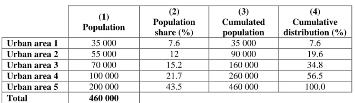
To develop the idea underlying our proposal, we shall first illustrate our approach using fictitious data as an example7. Table 1 gives the population of each of 5 urban areas in one of the territories under investigation.
Table 1 - Fictitious data (1) Population (2) Population share (%) (3) Cumulated population (4) Cumulative distribution (%) Urban area 1 35 000 7.6 35 000 7.6 Urban area 2 55 000 12 90 000 19.6 Urban area 3 70 000 15.2 160 000 34.8 Urban area 4 100 000 21.7 260 000 56.5 Urban area 5 200 000 43.5 460 000 100.0 Total 460 000 6
Although it may be challenging to define economically meaningful areas to compute the underlying population data.
7 The use of fictitious data is strictly for expositional convenience. In the Spanish data we use later on, provinces display a tight
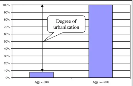
As mentioned before, a common measure of the degree of urbanization is the proportion of population living in urban areas above a certain size. For instance, given the data in Table 1, the degree of urbanization could be measured as the proportion of population living in urban areas with a population of at least 50 000. In our example this would be 92.4% (425 000 / 460 000). Referring to the cumulative distribution (Table 1, column 4), this way of measuring urbanization amounts to lumping together all categories but the first. The conventional measure of urbanization is therefore based on a highly simplified representation (Figure 1) of the more detailed distribution of population, represented in Figure 2.
Figure 1 – Cumulative distribution underlying the conventional measure of urbanization
Figure 2 – Cumulative distribution of population among urban areas 0% 10% 20% 30% 40% 50% 60% 70% 80% 90% 100% Agg. < 50 k Agg. >= 50 k 0% 10% 20% 30% 40% 50% 60% 70% 80% 90% 100%
Agglomeration 1 Agglomeration 2 Agglomeration 3 Agglomeration 4 Agglomeration 5 Degree of
urbanization
Degree of urbanization
In our example, the conventional degree of urbanization is the sum of population shares of all urban areas but the first (Table 1, column 2). We shall try to make use of the more detailed information given by the cumulative distribution in Figure 2. One way of doing so would be to take the sum of distances above each bar in Figure 2. Algebraically, let fi be the fraction of
population residing in the ith urban area (LLM), and let
i j j i f F 1 be the cumulative
distribution8. The sum of distances above the bars is given by:
5 2 5 5 5 4 5 3 5 2 4 1 5 1 5 1 1 5 1 1 1 1 i i i i i i i i i i i j i j i i j j i i f i f f f f f f F [1]It is a weighted sum of all urban area sizes except for the one that has a population below the urban threshold of 50 000; the weight of each urban area is its rank i minus 1.
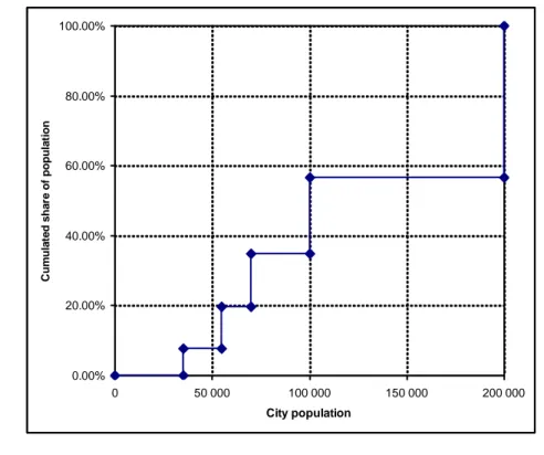
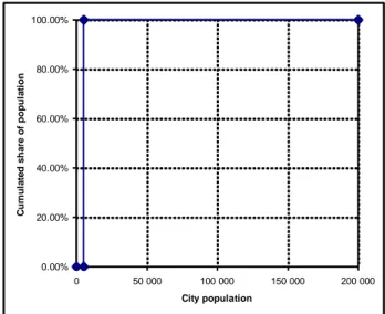
But note that the bar chart in Figure 2 does not reflect the relative sizes of urban areas. This is correctly taken into account in Figure 3.
Figure 3 – Cumulative distribution with city sizes on the X-axis
8 Of course, there is a different distribution for every territory (province), and a perfectly accurate notation would also have a
subscript for the province. Here, to simplify the notation, we omit the province subscript and retain only the LLM subscript.
0.00% 20.00% 40.00% 60.00% 80.00% 100.00% 0 50 000 100 000 150 000 200 000 City population C u m u la te d s h a re o f p o p u la ti o n
The measure of potential agglomeration economies which we formally develop below corresponds to the area above the cumulative distribution in Figure 3. This is remindful of the Gini coefficient which is equal to the area above the Lorenz curve9. But before proceeding, one last development is in order. A convenient measure of the degree of urbanization should vary from zero to 1, or 100%. In order to achieve this, we need some kind of normalization rule. One way of doing this is to rescale the horizontal axis of the cumulative distribution in terms of the size of the largest city in the urban system under study (in our application it will be Madrid). So let xi be the population size of urban area i, relative to the largest city in the urban system considered: system urban the in city largest the of Population area urban of Population i x i [2]
Define x0 = 0 and let N be the number of urban areas. As before,
N j j i N j j i i x x x x f 0 1 [3]is the fraction of population residing in the ith urban area (with f0 = 0), and
i j j i j j i f f F 0 1 is
the cumulative distribution (with F0 = 0). Urban areas are assumed to be ordered from smallest to largest. Our proposed index is:
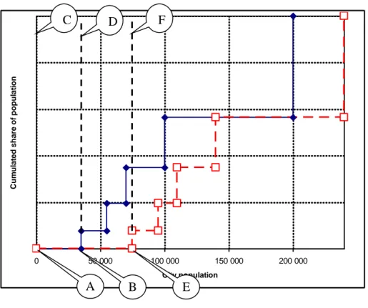
N i i i i x x F I 1 1 1 1 [4]Note that the first term of formula [4] is the area above the curve to the left of the first urban area in Figure 3. This implies that there is no threshold below which a populated area is considered non-urban. Deleting that first term would be an error, since it would result in an index that is insensitive to a horizontal shift in the cumulative distribution. In Figure 4, the blue line reproduces the distribution in Figure 3, while the red line represents a rightward shift in the distribution. If we do not count rectangles ABCD and AECF, the area above both distributions is the same, and so is the value of the index, whereas all urban areas in the shifted (red) distribution are larger. Of course, it would be possible to take into account a minimum urban size by
9
measuring the surface above the cumulative distribution only to the right of some threshold value (say, 50 000 inhabitants); but that would only make calculations messy. Moreover, it could be argued that there is some potential for agglomeration economies even in small villages.
Figure 4 – Cumulative distribution with city sizes on the X-axis
It is easily verified that our index weighs the population shares of urban areas according to their relative sizes. Equation [4] can be written as:
1)
N i i i i j j x x f I 1 1 1 0 1 [5] 2)
N i i i j j N i i N i i i j j N i i x f x x f x I 1 1 1 0 1 1 1 1 0 1 [6] 3)
N i i N i j j N i i N i j j x f x f I 1 1 1 [7] 0 50 000 100 000 150 000 200 000 City population C u m u la te d s h a re o f p o p u la ti o n B F C D A ERemebering that x0 = 0, 1)
N i i N i j j N i i N i j j x f x f I 2 1 1 [8] 2)
1 1 1 1 N i i N i j j N i i N i j j x f x f I [9] 3)
1 1 1 1 1 N i i N i j j N i i N i j j N Nx f x f x f I [10] 4)
1 1 1 N i i N i j j N i j j N Nx f f x f I [11] 5)
N i i i N i i i N Nx f x f x f I 1 1 1 [12]The formula in equation [12] has the merit of being much simpler and easier to compute than the one in equation [4]. In addition, formula [12] lends itself to the interpretation given in Arriaga (1970, p. 209)10: since fi is the probability that a randomly chosen individual reside in urban area i, then the average individual in the province lives in an urban area whose size is I times the size of the largest city in the urban system under study. Let us pursue the development, substituting from [3], 6)
N j j i N j j i i x x x x f 0 1 [3] we find: 7)
N j j N i i x f I 0 1 2 [13] 10Indeed, the proposed index is identical to the theoretical index proposed by Arriaga, except for its division by the population of the largest city in the urban system under study. Arriaga investigates the implications of using a truncated index which ignores the bottom end of the size distribution of agglomerations, and concludes that a truncated index is a good approximation, under mildly restrictive hypotheses. But in our case, there is no truncation, because the local labor markets (LLMs) cover the whole territory: see 3.1 below. Appendix I presents a version of the index that is based on information aggregated by size classes and therefore deals with truncation.
where: 8)
N i i f H 1 2 [14]is the HH index of concentration. So:
9) I x H N j j
0 [15]Our index is the HH index of concentration, multiplied by a factor that reflects the size of the province relative to the size of the largest city of the urban system considered (in our empirical application, Section 3, it will be the city of Madrid). In other words, our index accounts for both concentration and (relative) scale, which we consider as two aspects of the potential for economies of agglomeration. But, contrary to the HH index, its inverse does not have a straightforward interpretation11.
It is shown in the Appendix I that it would also be possible to compute the index, and obtain similar results, when the underlying population data is available only in city-size categories, rather than for each urban area. This is a strength of the proposal as it would allow comparing the potential for agglomeration economies of countries with different ways of providing the statistical information (in city-size categories or for each urban area) without affecting the index’s performance.
Boundary problem
So far, the proposed index has been developed under the assumption that every urban area (LLM) i is entirely contained in a single territory (province). But that is seldom true. In the Spanish case, several LLMs include some municipalities that are located in a different province. As before, we define fi as the fraction of population residing in the ith urban area. Given definition [2], 1) system urban the in city largest the of Population area urban of Population i x i [2]
11 Adelman’s (1969) has shown the “numbers-equivalent” property of the Hirchman-Herfindahl index (H): its inverse (1/H) can be
if only part of urban area i belongs to the territory under consideration, then equation [3] is no longer true, and
2)
N j j i i x x f 1 [16]However, bearing in mind Arriaga’s (1970) interpretation, the average (relative) size of the urban area where a randomly chosen individual lives is still given by formula [12]:
3)
N i i i N i i i N Nx f x f x f I 1 1 1 [12]But the tight relationship of our index with the HH concentration index breaks down.
In Section 3 below, our index combines the relative sizes xi of LLMs, and population shares fi computed at the scale of component municipalities, based on the province in which each municipality is actually located. In the Appendix II, this is compared with an index for which each LLM has been attributed in its entirety to the province where its centroid is located, which is tantamount to redrawing provincial boundaries. Interestingly, at least in the Spanish case, the two versions of the index are tightly correlated across the 52 provinces.
Properties of the index
The proposed index in non-negative, and its lower bound is zero. This extreme case would be approximated if all of the population lived in rural areas, in very small villages (of, say, 5 000 inhabitants); the curve would then be close to an upside-down «L», with the horizontal line at the 100% level, and the vertical line at the 5 000 population level, as illustrated in Figure 5.
Figure 5 – Cumulative distribution, no urbanization
The upper bound of the index is 1. This would correspond to a province whose population would be concentrated in a single urban area equal in size to the reference city, Madrid. The curve would then be a mirror-image of an «L», with the vertical bar to the right. Actually, this latter case is not too different from the Madrid province, where 98.2% of the population lives in the Madrid metropolitan area, as shown in Figure 6.
Figure 6 – Cumulative distribution, Madrid, 2001
0.00% 20.00% 40.00% 60.00% 80.00% 100.00% 0 50 000 100 000 150 000 200 000 City population C um ul a te d s ha re of po pu la ti on 0.00% 20.00% 40.00% 60.00% 80.00% 100.00% 0 1 000 2 000 3 000 4 000 5 000 6 000
City population (thousands)
C um ul a te d s ha re of po pu la ti on
A key property of the index is that it correctly reflects the change in the potential for agglomeration economies of any reallocation of population. This property is close to the Pigou-Dalton transfer principle for measures of inequality, which states that any change in the distribution that unambiguously reduces inequality must be reflected in a decrease in its measure. Let xi represent the change in the relative population size of urban area i. A reallocation of
population is restricted by the condition that 0
1
N i ix . Any reallocation can be represented as a
series of reallocations between two urban areas, and any reallocation between two urban areas can be represented as a series of reallocations between an urban area and the following or preceding one when urban areas are ordered according to size. Therefore, we need only to consider a reallocation of population from urban area s –1 to urban area s (from an urban area to the next higher ranking one in terms of size):
xs = –xs–1 > 0, and xi = 0 for i s, s–1 [17]
According to our theoretical a priori, such a reallocation raises the potential for agglomeration economies. What effect does it have on the index?
Following equation [3], define12:
N j j i N j j i i x x x x f 0 1 [18] where, in view of [17],
N j j s s N j j x x x x 1 1 1 [19] and 0 1 s s f f [20]The value of the index after the reallocation is:
12 The argument that follows can be generalized, albeit laboriously, to the version of the index that deals with the boundary problem.
s s
s s
s s
s s
s s i i i x x f f x x f f x f I
1, 1 1 [21] s s s s s s s s s s s s s s s s s s i i i x f x f x f x f x f x f x f x f x f I
1, 1 1 1 1 [22]
s s
s s
s s
s s s s s s s s i i i x f x x f x f f x f x f x f I
2 1 1 1 1 , 1 [23]
s s
s s
s s
s s N i i i x f x x f x f f x f I
1 1 2 1 [24]
fs fs
xs fs
xs xs
fs xs I I 2 1 1 [25]Given that the urban areas are ordered from the smallest to the largest, xs > xs–1, and fs > fs–1 , so that I' > I.
Another interesting property of the proposed index is that it lends itself to territorial aggregation or disaggregation. Consider partitioning a territory in such a way that agglomeration i belongs to subdivision A if iA, and to subdivision A if iA. Starting with formula [13], we have
N j j A i i N j j A i i x f x f I 0 2 0 2 [26]
A j j N j j A j j A i i A j j N j j A j j A i i x x x f x x x f I 2 0 2 0 [27] Now let
N j j A j j A x x F 0 [28]A i A j j N j j i A j j i A i F f x x f x x f
0 [29]And we can rewrite [27] as
A j A j A i A iA A j A j A i iA A F x F f F x F f I 1 1 1 1 2 2 [30]
A
A A AI F I F I 1 [31]The index of a territory is a weighted average of the indexes of its subterritories, where the weights are given by population shares.
Relationship with the Pareto distribution
The empirically estimated exponent of the Pareto city-size distribution (a generalization of Zipf’s rank-size rule) has been used as a measure of the concentration of an urban system (Rosen and Resnick, 1980). Following the notation established above, the (discrete) Pareto distribution can be written as: a i Ax i N1 [32]
where N is the number of cities (ranked from the smallest to the largest), xi is the size of city i 13, and A and a are parameters. Parameter A can be calibrated from the size of the largest city:
a N Ax N N1 1 [33] a N x A [34] Inverting [22], we obtain: i N A xia 1 [35] a i i N A x 1 1 [36]
Total urban population is:
13
N i a N i i N i A x X 1 1 1 1 [37]And so it is quite straightforward to construct a cumulative distribution similar to the one in Figure 3 reflecting a theoretical Pareto distribution. It is then possible to apply our proposed index to a theoretical Pareto distribution using formula [12]:
N i i i x f I 1 [12] There results
N i a N i a i N A i N A I 1 1 1 2 1 1 [38]where we exploit the identity14:
N j j N i i N i N i j j i N i i i x x x x x x f I 1 1 2 1 1 1 [39]If we assume that the number of cities N and the size of the largest city xN are fixed, then, using [34], [38] can be written as15:
N i a a N N i a a N i N x i N x I 1 1 1 2 1 1 [40] 14Here again, we ignore the boundary problem, which the Pareto distribution approach does not handle anyway.
15
N i a N N i a N i N x i N x I 1 1 1 2 2 1 1 1 1 [41]
N i a N i a N i N i N x I 1 1 1 2 1 1 1 1 [42]It is shown in the Appendix IV that the derivative of the index relative to the Pareto parameter is
2 1 1 1 1 1 2 1 1 2 2 1 ln ln 2 1
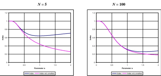
N i N j N i N j N i N a a a a a i i i j i i j a x a I [43]The sign of that derivative is the sign of its numerator, but we could not determine that sign analytically. Using numerical simulations16, we obtain that the derivative is negative for low values of a, and positive for high values. The sign reversal of the derivative is explained by the fact that, for a given number of cities, the size of the smallest city under the rank-size rule,
a N x x N 1 1
, increases with a, leaving a larger gap to the left of the first point on the cumulative distribution (see Figure 3). Referring to index computation formula [5],
N i i i i j j x x f I 1 1 1 0 1 [5]it is easily verified that its first term is equal to x1. Indeed, our numerical simulations confirm that, if that first term is omitted, our index is a monotonically decreasing function of parameter a. This is illustrated in Figure 7.
16
Figure 7 – Relationship of the proposed index to the Pareto elasticity parameter
N = 5 N = 100
EMPIRICAL APPLICATION
The Spanish provinces
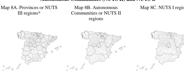
Administratively, Spain is divided into 8 105 municipalities that are aggregated into 52 provinces (NUTS III level) and seventeen Autonomous Communities or NUTS II regions (Figure 8 - Maps 8A and 8B). The number of municipalities within each province ranges from 34 (Las Palmas) to 371 (Burgos). Furthermore, there are Autonomous Communities with several provinces, for example, Andalusia with eight, and others with only one, like Asturias. For comparison with other European Union member-states, the seventeen Autonomous Communities can be aggregated into seven administrative regions or NUTS I regions (Figure 8, map 8C), which have no real internal political or administrative meaning.
0 0.2 0.4 0.6 0.8 1 1.2 0 0.5 1 1.5 2 Parameter a Ind e x
Index Index w/o smallest
0 0.2 0.4 0.6 0.8 1 1.2 0 0.5 1 1.5 2 Parameter a Ind e x
Figure 8 – Spanish administrative division of the territory into Provinces (NUTS III), Autonomous Communities (NUTS II) and NUTS I.
Map 8A. Provinces or NUTS III regions*
Map 8B. Autonomous Communities or NUTS II
regions
Map 8C. NUTS I regions
* Bold lines are provincial boundaries; fine lines are municipal boundaries. Source: Own.
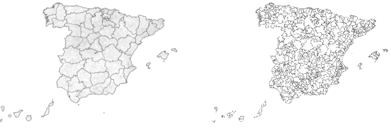
It is important to point out that we do not use municipalities as our territorial units of analysis (Figure 9 – map 9A). The municipality is an administrative division of the territory with no economic significance, because, in many cases, there is a high level of commuting between neighboring municipalities. An urban area could transcend municipal boundaries, to make up metropolitan areas, which might include several population nuclei surrounding a core one. To consider this fact, we aggregate the information offered by municipalities into LLMs. The regionalization method developed by Sforzi and Lorenzini (2002) and ISTAT (2006), applied to Spain by Boix and Galleto (2006), identifies the LLMs through a multi-stage process. Applying an algorithm that consists of four main stages and a fifth stage of fine-tuning, these authors aggregate the 8 106 Spanish municipalities into 806 LLMs. The algorithm starts with the municipal administrative unit and it generates the LLMs by using data of resident employed population, total employed population and displacements from the place of residence to the workplace, from the 2001 Spanish Population and Housing Census (INE)17. Map 9B shows the 806 LLMs defined by these authors18.
17
This is the most recent data as the 2011 Spanish Population and Housing Census (INE) is not yet available.
18 More details and applications of LLMs in Fernandez and Rubiera (2012). Rubiera and Viñuela (2012) perform an economic
Figure 9 – Spanish local areas: administrative basic unit (municipalities) and economic local unit (LLMs) (2001)
Map 9A. Spanish division of the territory into 8,105 municipalities*
Map 9B. Spanish division of the territory into 806 LLMs
* Bold lines are provincial boundaries; fine lines are municipal boundaries. Source: Own.
We have aggregated municipal employed population data from the 2001 Spanish Population and Housing Census (INE) to LLM data, following Boix and Galleto (2006). The LLM data are used to compute our index of potential agglomeration economies for each province. In the cases in which the LLM exceeds the limits of a province, we recalculate the part that belongs to each province, as proposed in Section 2.319. Then, for each province, we calculate the cumulative distribution of population according to the relative LLM size, in terms of the Madrid LLM, the biggest in the country.
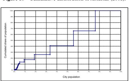
Figure 10 represents this cumulative distribution for the province of Asturias (being similar to Figure 3, but using real data and considering the LLM size as a percentage of that of Madrid). Next, the area above the curve of the cumulative distribution is calculated. In our example Asturias obtains the 82,6% level of the index.
19 Nevertheless, in Appendix 3, we also present the results assuming that the population of these special cases belongs to the
Figure 10 – Cumulative distribution of Asturias (2001). 0% 10% 20% 30% 40% 50% 60% 70% 80% 90% 100% 0% 1% 2% 3% 4% 5% 6% 7% 8% 9% 10% C u m u la te d s h a re o f p o p u la ti o n City population
Source: Own based on INE (2001) data.
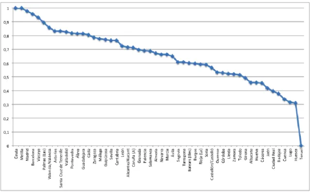
All the Spanish provinces are plotted in Figure 11, ranked by the value of the index. Madrid is followed by Barcelona and, at a much greater distance by Vizcaya, Valencia and Seville, which are among the biggest cities of the country. The rest of the distribution is intuitively reasonable, on the basis of our practical knowledge of the Spanish geographical economy.
Figure 11 – Proposed index, ranked in decreasing value, Spain (2001).
Index performance evaluation
Figure 12 plots the classical and HH measures of urbanization/concentration, the percentage of population living in cities of more than 50 000 inhabitants. Clearly, the values of our index (Figure 11) are very different and so, the ranking derived. Our index offers greater contrast, better reflecting the position of cities such as Barcelona or, less noticeably, Vizcaya, Valencia and Sevilla.
To illustrate how our index is able to better capture economic patterns, we correlate it with the
location quotients of some of the activities known to be highly sensitive to agglomeration
economies: high order producer services, also called knowledge intensive business services (henceforth KIBS). There are numerous empirical studies that confirm the relationship between agglomeration economies and this kind of services20. In this literature, the relationship between agglomeration economies and the concentration of these knowledge intensive services is clearly confirmed. Hence, we expect that the index which presents the highest correlation with the location quotients of these services is the one that better captures the potential for agglomeration economies.
The location quotient (LQ) that we use is the simplest one, defined as follows:
E E
e e LQ j i ji ji [44]where LQji is the location quotient of sector x in area a; eji is employment in sector j in province
i;
j ji
i e
e is total employment in spatial unit i;
n i ji j e E 1
is the total employment in sector j in Spain (n is the number of spatial units: 52 provinces). Finally,
j j
E
E is the total
employment in Spain.
Results of the correlations are computed for three indexes (the classical, the HH and our proposed one) and four examples of high order producer services: (i) financial services, (ii) computing and information technologies, (iii) advertising services and (iv) audiovisual and entertainment services. Nevertheless, the results are almost the same for all kinds of high order producer services. Our proposed index is presented in logarithms to obtain a better picture of the distribution among the provinces.
20
The reasons for the concentration of such services in large metropolitan areas are strongly connected with the presence of different types of effects directly derived from the existence of agglomeration economies. The diversity and rapidly changing nature of talents and know-how mean that only the largest cities will provide the necessary specialized labor pool. Such industries are, in other words, dependent on a constant stream of face-to-face meetings with a wide (and changing) range of individuals that only can occur in cities, but better in large cities. See Daniels (1985), Illeris (1996), Shearmur and Doloreux (2008), Polèse et al. (2007) or Wernerheim and Sharpe (2003), among many others.
Figure 12 – Classical and HH indexes ranked in decreasing order, Spain (2001).
Figure 12a – Classical Index
Figure 12b – HH Index
For all these activities, the proposed index captures much better the effect of the main metropolitan areas of the country: Madrid, represented by the top right-hand point in the trend lines, and Barcelona, the point in the middle of the trend lines. For the rest of the cities, this index clearly identifies the relationship between urbanization and agglomeration better than others. Table 2 shows the correlations among our proposed index and the classical way of measuring urbanization and the HH concentration index (as examples of other common procedures to capture urbanization or agglomeration effects). In all the cases, the highest correlations are obtained with our index.
Figure 13 illustrates these results. As can be seen, the classical index, in many cases, presents too much dispersion (not to mention heteroskedasticity) but, essentially, the biggest mistakes appear in the higher values of the index, that is, in the provinces where the biggest cities are. It gives almost the same value to Madrid, Barcelona, Ceuta and Melilla21. It is not capable of distinguishing between the biggest cities, especially Madrid but also Barcelona, and other cities of substantial but smaller size, such as Bilbao. The HH index works similarly to the classical one. It makes significant errors in the middle of the distribution in which there are cases of important concentration without a clear process of agglomeration, and vice versa. It also presents the problem found in the classical index for the top of the distribution.
The correlation of KIBS with our proposed index let us to clearly observe how it is able to perform well not only in those provinces with large cities but also in all those with small or medium sized cities. Indeed, the relationship between the location of KIBS and our index takes a clear curvilinear shape.
Table 2 - Correlations between the proposed, classical and HH indexes and KIBS (2001)
Telecommuni-cations Financial services Informatics and new technologies Research and development Advertising Audiovisual and entertainment Proposed index 0.83 0.76 0.85 0.79 0.89 0.84 Classical index 0.43 0.29 0.49 0.65 0.50 0.55 HH Index 0.47 0.29 0.50 0.54 0.36 0.48 Source: Own. 21
Figure 13 – Correlations between the proposed, the classical and the HH indexes
and KIBS LQs for the Spanish provinces (2001) (1)
Figure 13.1a – Correlation between the proposed index and financial services LQs
Figure 13.2a – Correlation between the classical urbanization index and financial services LQs
Figure 13.3a – Correlation between the HH concentration index and financial services LQs
Figure 13.1b – Correlation between the proposed index and computing and information technologies LQs
Figure 13.2b – Correlation between the classical urbanization index and computing and information
technologies LQs
Figure 13.3b – Correlation between the HH concentration index and computing and information
technologies LQs 0 0,2 0,4 0,6 0,8 1 1,2 1,4 1,6 1,8 0,01 0,1 1 LQ
Log (proposed index)
0 0,2 0,4 0,6 0,8 1 1,2 1,4 1,6 1,8 0 0,1 0,2 0,3 0,4 0,5 0,6 0,7 0,8 0,9 1 LQ Classical index 0 0,2 0,4 0,6 0,8 1 1,2 1,4 1,6 1,8 0 0,1 0,2 0,3 0,4 0,5 0,6 0,7 0,8 0,9 1 LQ HH 0 0,5 1 1,5 2 2,5 3 0,01 0,1 1 LQ
Log (proposed index)
-0,5 0 0,5 1 1,5 2 2,5 3 0 0,1 0,2 0,3 0,4 0,5 0,6 0,7 0,8 0,9 1 LQ Classical index 0 0,5 1 1,5 2 2,5 3 0 0,1 0,2 0,3 0,4 0,5 0,6 0,7 0,8 0,9 1 LQ HH
Figure 13.1c – Correlation between the proposed index and advertising services LQs
Figure 13.2c – Correlation between the classical urbanization index and advertising services LQs
Figure 13.3c – Correlation between the HH concentrationn index and advertising services LQs
Figure 13.1d – Correlation between the proposed index and audiovisual and entertainment services LQs
Figure 13.2d – Correlation between the classical urbanization index and audiovisual and entertainment
services LQs
Figure 13.3d – Correlation between the HH concentration index and audiovisual and
entertainment services LQs
Source: Own based on INE (2001) data.
(1)
The proposed index is expressed in logarithms.
0 0,5 1 1,5 2 2,5 3 0,01 0,1 1 LQ
Log (proposed index)
0 0,5 1 1,5 2 2,5 3 0 0,1 0,2 0,3 0,4 0,5 0,6 0,7 0,8 0,9 1 LQ Classical index 0 0,5 1 1,5 2 2,5 3 0 0,1 0,2 0,3 0,4 0,5 0,6 0,7 0,8 0,9 1 LQ HH 0 0,5 1 1,5 2 2,5 0,01 0,1 1 LQ
Log (proposed index)
0 0,5 1 1,5 2 2,5 0 0,1 0,2 0,3 0,4 0,5 0,6 0,7 0,8 0,9 1 LQ Classical index 0 0,5 1 1,5 2 2,5 0 0,1 0,2 0,3 0,4 0,5 0,6 0,7 0,8 0,9 1 LQ HH
SUMMARY AND CONCLUSIONS
Urbanization is, undoubtedly, a crucial phenomenon in the processes of economic and social development and industry specialization of a territory. It is commonplace to say that cities form and grow to exploit economies of agglomeration. Consequently, there is a need in empirical spatial analysis for some type of variable that informs about agglomeration economies. What is typically measured is agglomeration itself (for instance, when the unit of analysis is the individual urban area, city population, or employment). A measure of agglomeration is not a measure of agglomeration economies, but rather a measure of the potential for agglomeration economies. However, the usual ways of measuring agglomeration in a territory are not entirely satisfactory.
In this paper, we develop an index with several desirable properties. It has a graphical representation that is closely analogous to the development of the Gini coefficient from the Lorenz curve and can be formulated as an extension of the HH concentration index. It varies between 0 and 1, conforms to a version of the Pigou-Dalton transfer principle, and lends itself to territorial aggregation and disaggregation. It can be related to the elasticity parameter of the Pareto distribution, a generalization of Zipf’s rank-size rule.
In our empirical illustration, we apply our index to the Spanish provinces (NUTS III regions) using local labor markets as the basic units for its construction, instead of administrative territorial divisions such as municipalities. Our index offers a much more credible and contrasted ranking than other classical ways of measuring the potential agglomeration economies of a territory. We look forward to applying our proposed index to other countries, such as the US and its counties.
The index could be very valuable for any descriptive or econometric analysis for a single country or for cross-country comparisons. Furthermore, it is a useful tool that could be used to enhance a more suitable design of economic policies.
REFERENCES
ADELMAN, M. A. (1969) “Comment on the “H” Concentration Measure as a Numbers-Equivalent”, The Review of Economics and Statistics, 51(1), pp. 99-101.
ADES, F. and E. L. GLAESER (1995) “Trade and circuses: explaining urban giants”, Quarterly Journal of Economics, 110, pp. 195-227.
ARBIA, G. (1989) Spatial data configuration in statistical analysis of regional economic and related problems. Dordrecht, Netherlands: Kluwer.
ARRIAGA, E. E. (1970) “A new approach to the measurements of urbanization”, Economic Development and Cultural Change, 18(2), pp. 206-218.
BEARDSELL, M. and V. HENDERSON (1999) “Spatial evolution of the computer industry in the USA”, European Economic Review, 43, pp. 431-56.
BOIX, R. and V. GALLETO (2006) Identificación de Sistemas Locales de Trabajo y Distritos Industriales en España. Dirección General de Política de la Pequeña y Mediana Empresa, Ministerio de Industria, Comercio y Turismo.
BRÜLHART, M. and F. SBERGAMI (2009) “Agglomeration and growth: cross-country evidence”, Journal of Urban Economics, 65, pp. 48-63.
CICCONE, A. and R. E. HALL (1976) “Productivity and the density of economic activity”, American Economic Review, 86(1), pp. 54-70.
DANIELS, P. (1985) Service Industries: A geographical Perspective. New York, Methuen.
DURANTON, G. and D. PUGA (2002) “Diversity Specialization in Cities: Why, Where and Does it Matter”, in P. MCCANN (Ed.): Industrial Localization Economics, pp. 151-186. Cheltenham-Edward Elgar. FAY, M. and C. OPAL (2000) Urbanization without growth: a not so uncommon phenomenon. Working
Paper No. 2412, The World Bank, Washington, DC.
FERNÁNDEZ, E. and F. RUBIERA (2012) Defining the Spatial Scale in Modern Economic Analysis: New Challenges from Data at Local Level. Advances in Spatial Science Series. Springer.
FOTHERINGHAM, A. S. and D. W. S. WONG (1991) “The modifiable areal unit problem in multivariate statistical-analysis”, Environment and Planning A, 23, pp. 1025-1044.
GLAESER, E. L. (1994) “Cities, information, and economic growth”, Cityscape, 1(1), pp. 9-77. GLAESER, E.L. (1998) “Are Cities Dying?”, Journal of Economics Perspectives, 12(2), pp. 139-160. HALL, P. (2000) “Creative cities and economic development”, Urban Studies, 37(4), pp. 639-649.
HENDERSON, V. (1988) Urban Development: Theory, Fact and Illusion. New York: Oxford University Press.
HENDERSON, V. (2003) “Marshall’s scale economies”, Journal of Urban Economics, 53, pp. 1-28. INE (2001) Censo de Población, 2001. Instituto Nacional de Estadística (www.ine.es).
ILLERIS, S. (1996) The service economy: A geographical approach. Chichester, U.K., Wiley. ISTAT (2006) Distretti Industriali e Sistemi Locali del Lavoro 2001. Collana Censimenti. JACOBS, J. (1969) The Economy of Cities, Vintage, New York.
JACOBS, J. (1984) Cities and the wealth of nations, Vintage, New York.
JONES, B. and S. KONÉ (1996) “An exploration of relationships between urbanization and per capita income: United States and countries of the world”, Papers in Regional Science, 75(2), pp. 135-153. KRUGMAN, P.R. (1991) “Increasing Returns and Economic Geography”, Journal of Political Economy, 99,
LEMELIN, A. and M. POLÈSE (1995) “What about the bell-shaped relationship between primacy and development?” International Regional Science Review, 18, pp. 313-330.
LONG, L. and A. NUCCI (1997) “The Hoover index of population concentration: a correction and update”, The Professional Geographer, 49, pp. 431- 440.
OPENSHAW, S., and P. J. TAYLOR (1981) “The modifiable areal unit problem”, in N. WRIGLEY and R. J. BENNETT (Eds.) Quantitative geography, pp. 60-70. London: Routledge.
PAELINCK, J. H. P (2000) “On aggregation in spatial econometric modeling”. Journal of Geographical Systems 2, pp. 157–165.
PETERSEN, G. (1991) Urban economies and national development. Office of Housing and Urban Programs, USAID, Washington, DC.
POLÈSE M., R. SHEARMUR and F. RUBIERA (2007) “Observing regularities in location patters. An analysis of the spatial distribution of economic activity in Spain”, European Urban & Regional Studies, 14(2), pp. 157-180.
PORTER, M. (1990) The competitive advantage of nations, Free Press, New York.
PRUD´HOMME, R. (1997) “Urban transportation and economic development”, Région et Développement, 5, pp. 40–53.
QUIGLEY, J.M. (1998) “Urban Diversity and Economic Growth”. Journal of Economic Perspectives, 12(2), pp. 127-138.
RICHARDSON S. (1992) “Statistical methods for geographical correlation studies”. In: ELLIOT P, CUZICK J., ENGLISH D., STERN R. (Eds.) Geographical and environmental epidemiology: methods for small area studies. Oxford University Press, New York, pp. 181-204.
ROBINSON W.S. (1950) “Ecological correlations and the behaviour of individuals”, American. Sociological Review, 15, pp. 351-357.
ROSEN, K. and M. RESNICK (1980) “The size distribution of cities: an examination of the Pareto Law and Primacy”, Journal of Urban Economics, 8, pp. 165-186.
ROSENTHAL, S. S. and C. W. STRANGE (2001) “The determinants of agglomeration”, Journal of Urban Economics, 50(2), pp. 191-229.
RUBIERA, F. and A. VIÑUELA (2012) “From funtional areas to analytical regions, where the agglomeration economies make sense”, in FERNÁNDEZ, E. and F. RUBIERA, (Eds.) Defining the Spatial Scale in Modern Economic Analysis: New Challenges from Data at Local Level. Springer. SFORZI, F. and F. LORENZINI (2002) “I distretti industriali”, L´esperienza Italiana dei Distretti Industriali.
Instituto per la Promozione Indistriale (IPI).
SHEARMUR, R. and D. DOLOREUX (2008) “Urban hierarchy or local milieu? High-order producer service and (or) knowledge-intensive business service location in Canada, 1991-2001”. Professional Geographer, 60 (3), pp. 333-355.
UCHIDA, H. and A. NELSON (2010) “Agglomeration Index: Towards a New Measure of Urban Concentration”, in J. BEALL, B. GUHA-KHASNOBIS, and R. KANBUR (Eds.) Urbanization and Development, Oxford University Press.
WERNERHEIM, M. and C. SHARPE (2003) “High-order producer services in Metropolitan Canada: Howe footloose are they?”, Regional Studies, 37, pp. 469-90.
WHEATON, W. and H. SHISHIDO (1981) “Urban concentration, agglomeration economies, and the level of economic development”, Economic Development and Cultural Change, 30, pp. 17-30.
WORLD BANK (1991) Urban policy and economic development: an agenda for the 1990s. The World Bank, Washington, DC.