Numerical and Computational Strategy for Pressure-Driven Steady-State Simulation of Oilfield Production

To link to this article : DOI:10.1016/j.compchemeng.2008.09.007 URL : http://dx.doi.org/10.1016/j.compchemeng.2008.09.007

To cite this version : Floquet, Pascal and Joulia, Xavier and Vacher, Alain and Gainville, Martin and Pons, Michel ( 2009) Numerical and Computational Strategy for Pressure-Driven Steady-State Simulation of Oilfield Production. Computers & Chemical Engineering, vol. 33 (n° 3). pp. 660-669. ISSN 0098-1354

O

pen

A

rchive

T

OULOUSE

A

rchive

O

uverte (

OATAO

)

This is an author-deposited version published in : http://oatao.univ-toulouse.fr/ Eprints ID : 1110

Any correspondance concerning this service should be sent to the repository administrator: staff-oatao@inp-toulouse.fr.

Numerical and Computational Strategy for Pressure-Driven

Steady-State Simulation of Oilfield Production

Pascal Floquet(a), Xavier Joulia(a), Alain Vacher(b), Martin Gainville(c), Michel Pons(d)

a

Laboratoire de Génie Chimique (LGC), UMR-CNRS 5503, INPT-ENSIACET, 118, route de Narbonne, 31077 Toulouse Cedex 4 France. Pascal.Floquet@ensiacet.fr, Xavier.Joulia@ensiacet.fr

b

ProSim, Stratège Bâtiment A, BP 2738, F-31312 Labège Cedex France. Alain.Vacher@prosim.net c

IFP Direction Mécanique Appliquée, IFP-Rueil, 1-4 avenue de Bois Préau, 92852 Rueil-Malmaison Cedex France. Martin.GAINVILLE@ifp.fr

d

Michel Pons Technologie, 32, rue Raulin, F-69007 Lyon, France. michelpons.mpt@tiscali.fr

Abstract

Within the TINA (Transient Integrated Network Analysis) research project and in partnership with Total, IFP is developing a new generation of simulation tool for flow assurance studies. This integrated simulation software will be able to perform multiphase simulations from the wellbore to the surface facilities. The purpose of this paper is to define, in a CAPE-OPEN compliant environment, a numerical and computational strategy for solving pressure-driven steady-state simulation problems, i.e. pure simulation and design problems, in the specific context of hydrocarbon production and transport from the wellbore to the surface facilities.

Keywords

Pressure-driven simulation, Oilfield, CAPE-OPEN

1 Introduction

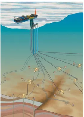
Usually, a deep water production system is constituted by a main field with links to satellite fields. The infrastructure of the system is made of subsea wellhead clusters, chokes, manifolds, production lines, risers and surface process units for separating liquid (water, oil) and gas phases (figure 1).

INSERT FIGURE 1

Figure 1: Deep Water Production System

This paper is divided into four parts. The first part introduces the well-known concepts of simultaneous modular steady-state simulation strategy and how to formulate and solve pressure-driven simulation problems. Indeed, in a pressure-driven process model, flowrates are such as pressure equality is satisfied at each manifold and mixing point (node) of the flowsheet. The second and third parts of this study are devoted to simulation and design problems solved in two representative cases: without material stream recycle and with recycle of compressed gas to the bottom of the riser (gas-lift) or of the wells. These basic cases are modeling different operating periods of an oil and gas production system; the first case corresponds to the beginning of a field operation, the other ones to the case of the activation of “non-eruptive” wells with riser top pressure constraint. The steady-state process simulator ProSimPlus™ is used to perform all these case studies. In the last part of this paper, CAPE tools interoperability is demonstrated through an industrial application: the ProSimPlus™ SPEC module (design specifications and recycle streams solver) on the one hand and the IFP multiphase pipe module on the other hand are

used as CAPE-OPEN compliant Unit Operations and integrated in the INDISS-TINA dynamic simulation tool.

2 Problem Statement and Pressure-Driven Steady-State

Simulation

The first purpose of this study is to prove the feasibility to extend the simultaneous modular strategy [Joulia et al., 1985], via ProSimPlus™ simulator and IFP process data, for solving steady-state pressure-driven simulation and design problems of oil and gas production networks. To perform this step, we have defined three base cases [1]-[3], represented in figure 2, 3 and 4 respectively.

2.1

Description of the base cases

INSERT FIGURE 2 to 4 Figure 2: Base Case [1] Figure 3: Base Case [2], gas-lift Figure 4: Base Case [3], pumping

All the flowsheets include two subsea production clusters constituted by respectively two and three subsea wells. Well flows are controlled by choking wellhead valves, named chokes. Clusters are connected together by a subsea flow line and a second flow line, connected to a riser, transports the production up to surface facilities. Manifolds are used to connect the flow lines. Finally, a basic surface process (flash drum) is used to separate liquid and gas phases and gas is compressed.

Each wellbore is known in terms of temperature T, pressure P and molar fractions z. Table 1 gives the data, T, P, gas-oil ratio (GOR) and water cut (WC), allowing to define the gas-oil-water fluids of the five wells. Compositional calculations have been performed using 9 pure components, including water, and 6 pseudo-components. For each well, the reference composition has been tuned to match the specified GOR and Water Cut reported in table 1. Finally, table 2 gives the characteristics of the pipelines of the network and specifies the flow regimes. To completely saturate the degrees of freedom of system and to be able to simulate the oilfield production, only the values of the openings, or pressure drops, of the chokes and the riser top pressure must be specified.

INSERT TABLES 1 to 2

Table 1: Data of the 5 wells for the case studies Table 2: Characteristics of the pipelines

Three main base cases have been defined: flowsheet without recycle (base case [1], figure 2), with recycle of gas from the riser top to the riser bottom (gas-lift or base case [2], figure 3) and with recycle of gas from the riser top to well bottoms (base case [3], figure 4). For each base case several simulation and design problems are considered.

2.2

Extension of the simultaneous modular approach

In a sequential modular simulator, such as Aspen Plus™, Chemcad™, PRO/II™, ProSimPlus™, the set of variables X° (temperature T, pressure P, molar fractions z and total flowrate F) defining the process feeds and the operating and design parameters  of the modules constitutes the standard input data of a pure simulation problem. In case of pressure-driven simulation problem, only the intensive variables (T,

P and z), which define the reservoir states at the wellbore bottoms, belong to the input data; well total

flowrates must be calculated in order to satisfy the following connection constraints: “all the connected input ports of a same manifold have the same pressure”.

INSERT FIGURE 5

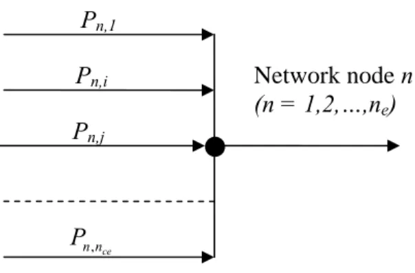
Figure 5: Hydraulic network node

Thus, each node (manifold) of the hydraulic network (figure 5) adds (nce–1) equality constraints, where

nce is the number of input streams of the node. These pressure equality constraints are the following:

(Pn,i – Pn,j)/P= 0 j > i; i = 1,2,…,(nce-1); j = 2,…,nce; n = 1,2,…,ne

where ne is the total number of the network nodes and Pa reference pressure. Note that the total number of pressure equality constraints is equal to (nw–1), where nw is the total number of wells. The last constraint, written for saturating the nw degrees of freedom corresponding to the well total flowrates, is the design specification on the riser top pressure.

From a numerical strategy point of view, a pressure-driven problem can be seen as a particular case of a design problem defined as: some degrees of freedom are saturated by design specification equations, instead of standard input data, and an equivalent number of variables belonging to X° or  is transferred from the input data set to the set of unknowns. These additional unknowns are called action variables. The physical action variables associated to pressure constraints are the well flowrates, but other variables can be chosen to satisfy pressure equalities, depending on the design problem type. For each basic case, without and with recycle, two types of problems are defined:

 Flowrates/Pressure (FP) problems in which well flowrates and riser top pressure are fixed and action variables, chosen among chokes (valves) openings or well pressures, are adjusted to verify pressure equalities at each manifold as well as the riser top pressure constraint.

 Pressures/Pressure (PP) problems in which well pressures and riser top pressure are fixed and only the well flowrates are action variables, for the same set of constraints.

For all cases studied (with or without recycle) the constraints of pressure equilibrium at each manifold are imposed and the riser top pressure is specified.

In ProSimPlus™, design problems are solved according to the simultaneous modular approach. Modular means that the process model is represented by an oriented graph, called simulation diagram, where each node corresponds to a module and each arc to a material or information stream. As illustrative example, the ProSimPlusTM simulation diagram of base case [3] problem is shown in figure 6. A short description of the used modules is given in appendix.

INSERT FIGURE 6

Figure 6: ProSimPlus™ simulation diagram of base case [3]

The graph is partitioned into sub-systems, single module or MCN (Maximum Cyclic Network), which can be solved sequentially, the ones after the others according to an order which follows the direction of flow of the process material streams. For each MCN, a numerical strategy must be implemented. This strategy consists of defining a set of torn streams (recycles) and the associated calculation order of the modules belonging to the MCN. At the MCN level, the numerical problem comes down to solving the following non-linear algebraic equations system:

h(x) = 0

Vectors h and x have two sources of elements:

- equations f and variables Z associated to torn streams :

Z is the set of estimated values of the independent variables (temperature, pressure and

partial molar flowrates) associated to the nt torn streams;g is the set of calculated values of these same variables by sequential passage thought the modules of the MCN.

- and design specifications equations d, among which the pressure equality constraints, and associated action variables s

d(Z,s) = 0

The dimension of the system is equal to [(nc+2)nt + ns], where nc is the number of components, nt the number of torn streams and ns ≥ nw the number of action variables.

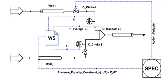
All these MCN level equations are simultaneously solved by a general non-linear algebraic equations solver, the SPEC module. Information streams are used on the one hand by SPEC for acting on module parameters (choke pressure drop, well pressure or flowrate) and on the other hand for transferring residues on design specification equations (pressure constraints from the manifolds and specification on the riser top pressure) back to SPEC. As an illustration, the graph associated to one pressure equality constraint and the corresponding action variable, the choke pressure drop, is presented on figure 7.

INSERT FIGURE 7

Figure 7: ProSimPlus™ simulation diagram associated to one constraint and one action variable

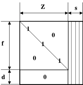
Among the available numerical methods, the Broyden-Identity (BRI) method proved to be the most efficient. In this method, a Jacobian approximation M(k) is generated at iteration k by the recurrence formula proposed by Broyden [Broyden, 1965; Broyden, 1969]. The initial matrix M(0) isshown on figure 8.

INSERT FIGURE 8

Figure 8: Initial matrix of the Broyden-Identity (BRI) method

As initialization, part of the Jacobian associated to recycle equations and variables is simply approximated by identity matrix. Columns associated to action variables are generated by numerical sensitivity. To avoid singular initial matrix, torn streams must be chosen such as they do not tear the way(s) which, by going all over the calculation graph, connect the action variables to specification equations.

Convergence is obtained when the criterion defined as:

 

_{ }

 

_{ }

_



 



is less than 10-8. i are weighting factors. In the first term, the weighting consists in dividing each difference between estimated (Zi,j) and calculated (gi,j) values by the mean value of these values.

3 Case Studies without recycle

3.1 Flowrates/pressure problems

For the first FP problem, which corresponds to base case [1] (figure 2), action variables are defined as the pressure drops of the five chokes and initialized to zero.

The convergence is obtained in 4 iterations and only 11 MCN simulations using the Broyden-Identity (BRI) method for a specification of 15 bar for the pressure at riser top. Generally speaking, the MCN simulations correspond to 2 successive substitutions as initialization of the iterative process, ns passages through the MCN for the generation of the right hand side columns in the initial M(0) of the BRI method and, if the relaxation procedure is not active, the number of iterations. For this first problem, ns = nw =5, then the number of MCN simulations is: 2 + 5 + 4 = 11

Figure 9 shows the results obtained for various specifications of the riser top pressure. From this figure, it can be deducted that well 2 is the less “eruptive” one. The eruptivity limit corresponds to the first null value of pressure drop (choke completely open), when the pressure specification increases. It can also be shown that a riser top pressure higher than 25 bar is physically impossible to reach without activation system such as gas-lift or pumping. Note that negative values for the pressure drops are allowed in the simulations to ensure the activation of the constraints. Well evidently it is physically impossible but it is a simple way for determining the less “eruptive” well.

INSERT FIGURE 9

Figure 9: Choke pressure drops function of riser top pressure (Base case [1], FP problem 1)

Another FP problems have been solved, in which the action variables are the four pressure drops of the chokes associated to the more eruptive wells and the flowrate of the less eruptive one (i.e. well 2, with choke 2 completely open, for this case). The convergence is now obtained in 6 iterations and 13 MCN simulations, with the same numerical method (BRI) and specifications as previously. Table 3 shows detailed results of this FP problem.

INSERT TABLE 3

Table 3: Detailed result of the 2nd FP Problem – Base Case [1]

For the last case of FP problems, the action variables are the five well bottom pressures for fixed choke pressure drops. For a specification of 15 bar for the pressure at riser top, the convergence is obtained in 5 iterations and 12 MCN simulations.

3.2 Pressures/Pressure problems

The last case without recycle solved consists in a PP problem. The action variables are the well flowrates for fixed choke pressure drops, respectively to 55, 25, 60, 40 and 50 bar. The convergence is obtained in 5 iterations and 12 MCN simulations. Note that this case can sometimes diverge, because of pressure drops specifications that may induce physical impossibility to balance pressures at the manifolds. Moreover, initialization of the well flowrates has a high impact on convergence. In figure 10, we can see flowrates of the five wells versus the riser top pressure specification.

INSERT FIGURE 10

Figure 10: Well flowrates function of the riser top pressure (Base case [1], PP problem)

4 Case Studies with recycle

When a riser top pressure specification is physically impossible to reach, two activation systems can be used: gas-lift, which consists to recycle gas from the output of the compressor to the bottom of the riser, or pumping which consists to recycle gas from the output of the compressor to the bottom of the wells.

Two types of problems, FP and PP, have also been solved with gas-lift (figure 3). The associated ProSimPlusTM simulation diagrams have two MCN. One upstream with action, for the first problem type, on the pressure drops of the four chokes associated to the most eruptive wells for balancing the pressures at the manifolds; the choke associated to the less eruptive well is completely open. The other MCN downstream with the gas recycle to the riser bottom (gas-lift) and action on flowrate, or split fraction, of recycle to the riser bottom to satisfy the specification on riser top pressure. The two MCN can be solved sequentially or simultaneously and convergence is easily obtained in the two cases. For example, only 5 iterations and 12 MCN simulations are necessary for the simultaneous strategy. Figure 11 shows typical results in which we can see that there is no need for gas-lift under a threshold of approximately 25 bar.

INSERT FIGURE 11

Figure 11: Gas-lift flowrate function of the riser top pressure specification (Base Case [2], FP problem)

For the second problem type, PP, the action variables are the well flowrates of the four most eruptive wells, for fixed choke pressure drops, and the flowrate of recycle (gas-lift) to the riser bottom. Same convergence difficulties, as in the case without recycle, due to possible unphysical specifications have been observed. The obtained results in terms of the evolution of gas-lift flowrate in function of riser top pressure specification are similar to the previous case (figure 11).

4.2 Recycle at the bottom of the wells (figures 4 and 6)

Another kind of activation consists on recycling gas at the bottom of the wells (figure 4). Here, FP and PP strategies can also be studied. The associated ProSimPlusTM simulation diagrams have only one MCN including all the modules (figure 6).

In the first case, action variables are the pressure drops of the four chokes of the most eruptive wells and the recycle ratio, with assumption of equal repartition on the five wells. Constraints are the same as previously: the manifold pressure balances and the specification of pressure at riser top. Although this problem is numerically more complex, convergence is reached in 13 iterations and only 20 MCN simulations. Figure 12 shows action variables versus riser top pressure specification.

INSERT FIGURE 12

Figure 12: Recycle ratio and pressure drops of the chokes function of riser top pressure (Base Case [3] – FP problem)

The PP strategy, in which well flowrates are all considered as action variables, gives the same type of results.

Table 4 sums up the results of all numerical performance tests in terms of number of pipe calculations. That is the key point for the CPU time criterion to be minimized, because, as described in the next section, these pipe modules are calculated, in the final version of the simulation environment, by the way of CFD approach which is very time consuming.

INSERT TABLE 4 Table 4: Sum up of the results

5 CAPE-OPEN integration

The ProSimPlus™ SPEC module (design specifications and recycle equations solver) and the IFP pipeline multiphase flow module (PPipe) have been made compliant with CAPE-OPEN (CO) Unit Operation 1.0 interface. PPipe is a rigorous steady-state pipe module based on a 1D Computational Fluid

Dynamics approach [Pauchon et al., 1993; Henriot et al., 1997]. Both SPEC and PPipe are integrated in INDISS-TINA environment as CO compliant Unit Operations. INDISS™ is the dynamic simulation platform chosen by TINA to provide a consistent set of data along the fluid line from wellbore to export facilities. INDISS™ is developed by RSI and respects the CAPE-OPEN standard for thermodynamic property servers, like Simulis® Thermodynamics, as well as for static and dynamic unit operations [Roux and Paen, 2005]. Some specific developments have been implemented within INDISS™ to order sequential calculations and to deal with the ProSimPlus™ SPEC module for simultaneously solving equations associated to design specifications and recycle streams: the calculation list of modules must be supplied to INDISS™ and information streams are shared between ProSimPlus™ SPEC and INDISS™. The previous simulations performed with ProSimPlus™, as feasibility study and numerical performance assessment, can now be performed with INDISS-TINA by using the CO-SPEC and CO-PPipe modules. In this way the pressure-driven steady-state simulation of oilfield production is carried out with efficiency and accuracy thanks to the combination, on the basis of the CAPE-OPEN standard, of the numerical, computational and hydrodynamic skills of the project partners in a unique software environment.

As illustration, figure 13 shows the results obtained with INDISS-TINA on the previous specified base case [2] – FP problem.

INSERT FIGURE 13

Figure 13: INDISS-TINA results from various riser top pressure specifications Base Case [2] – FP problem

The main difference between results from ProSimPlus™ and results from TINA are due to the different pipe modules used and well fluid characterizations. As example, for base case [2] – FP problem, the riser top pressure threshold, below which well 2 is not eruptive, varies from 25 bar (figure 11) to about 30 bar (figure 13).

Figure 14 illustrates the capability of integration via CAPE OPEN standard of IFP multiphase pipe modules and SPEC module into the INDISS™ environment.

INSERT FIGURE 14

Figure 14: CAPE OPEN Integration of CO-SPEC and CO-PPipe in INDISS™ environment

6 Conclusion

This study pointed out two major objectives. First, to check, through a series of twelve case studies, that a standard simulator based on modular approach and sequential resolution is able to efficiently solve steady state simulation and design problems of oil production and transport networks from wells to surface process. The proposed strategy is a simple extension of the simultaneous modular approach where pressure balances equations are added to classical design specification equations and simultaneously solved with recycle equations. In this way, classical CAPE simulators, such as ProSimPlus™, are able to solve efficiently pressure-driven steady-state simulation problems encountered in oil & gas production. The second objective was to check the interoperability of various software components for combining skills in various fields, oil, numerics and fluid mechanics, and so to solve complex interdisciplinary problems. The CAPE-OPEN standard appears as an excellent way to “plug and play” software components from various sources. In our application, two CAPE-OPEN compliant Unit Operations, the ProSimPlus™ SPEC module -“design specifications and recycle equations solver”- and the IFP Ppipe module -“pipeline multiphase flow module”- are integrated in INDISS-TINA environment as CO compliant Unit Operations. Future work concerns multi-period optimization and dynamic simulation problems.

References

Broyden G.C., A class of methods for solving nonlinear simultaneous equations, Math. Comp., 19, 577-593 (1965)

Broyden G.C., A new method of solving nonlinear simultaneous equations, Comp. J., 12, 94-99 (1969) Henriot V., Pauchon C., Duchet-Suchaux P. and Leibovici C., TACITE: Contribution of Fluid

Composition Tracking on Transient Multiphase Flow, Offshore Technology Conference (n° 8563),

Houston (1997)

Joulia X., Koehret B., Enjalbert M., Simulateur modulaire séquentiel à convergence simultanée, The Chem. Eng. Journal, 30, 3, 113-127 (1985)

Pauchon C., Dhulesia H., Lopez D. and Fabre J., TACITE: A Comprehensive Mechanistic Model for

Two-Phase Flow, 6th BHRG Multiphase International Conference 1993, Cannes, France, June (1993)

Roux P., Paen D., TINA Project, Transient Integrated Network Analysis, 10th CO-LaN annual meeting Come (2005)

APPENDIX – Short description of the ProSimPlus

Modules.

Only functionalities used in the presented examples are described.

Module Short description of the functionality used in base cases

Parameter(s) Icon

COMPRESSOR

Mono-stage compressor. Calculate the power required to compress an input vapour stream to a specified discharge pressure.

- Discharge pressure

- Isentropic yield

FLASH Adiabatic liquid-vapor flash - Pressure

MEASURE

Allow to measure (extract) a value (temperature, pressure, partial flowrates, composition …) from a steam. Used here for measuring the pressure of streams and transferring these values to SPEC or WS module via information streams.

- No

MIXER

The mixer module carries out the adiabatic mixture of ni input streams. It calculates the temperature and the physical state of the resulting stream by an adiabatic flash calculation. For this application, the output pressure is given by an information stream.

- Output pressure

PIPE

Pipe module calculates the pressure drop of a fluid in an isothermal pipe that can combine linear segments and accidents, described by their topology (length, difference in height,…) , characteristics (roughness, diameter,..) and flow regime (annular, dispersed, stratified,…).

- Topology and characteristics of the pipe: length, difference in height, diameter, roughness - Flow regime

SPEC

Non-linear equations solver used for the simultaneous solution of design specifications and recycle streams equations. Residues on equations are transferred to SPEC by information streams and SPEC acts on modules parameters by information streams too.

- Numerical parameters

SPLITTER

The splitter module divides an input stream to no output streams of same composition, temperature and pressure. It is the simplest module of a simulator.

- Split fractions of the (no-1) first output streams

VALVE Isenthalpic flash - Pressure drop

WS

WS is the acronym of Windows Script. It allows the user to create his own module, written in Visual Basic (VBScript). WS is used here for formulating the pressure constraints at the manifolds. - No SPEC SPEC WS WS

List of Figures

Figure 1: Deep Water Production System Figure 2: Base Case [1]

Figure 3: Base Case [2], gas-lift Figure 4: Base Case [3], pumping Figure 5: Hydraulic network node

Figure 6: ProSimPlus™ simulation diagram of base case [3]

Figure 7: ProSimPlus™ simulation diagram associated to one pressure equality constraint and one action variable

Figure 8: Initial matrix of the Broyden – Identity (BRI) method

Figure 9: Choke pressure drops function of riser top pressure (Base Case [1], FP problem 1) Figure 10: Well flowrates function of the riser top pressure (Base Case [1], PP problem)

Figure 11: Gas-lift flowrate function of the riser top pressure specification (Base case [2], FP problem) Figure 12: Recycle ratio and pressure drops of the chokes function of riser top pressure (Base case [3], FP problem)

Figure 13: INDISS-TINA results from various riser top pressure specifications (Base case [2] – FP problem)

Figure 14: CAPE OPEN Integration of CO-SPEC and CO-PPipe in INDISS™ environment

List of Tables

Table 1: Data of the 5 wells for the case studies Table 2: Characteristics of the pipelines

Table 3: Detailed result of the 2nd FP Problem – Base Case [1] Table 4: Sum up of the results

Cluster 1 Cluster 2 Choke 1 Choke 2 Choke 3 Choke 4 Choke 5 Well 1 Well 2 Well 3 Well 4 Well 5 Line 1 Line 2 Flash Compressor Ri ser Manifold Cluster 1 Cluster 2 Choke 1 Choke 2 Choke 3 Choke 4 Choke 5 Well 1 Well 2 Well 3 Well 4 Well 5 Line 1 Line 2 Flash Compressor Ri ser Manifold Manifold

Cluster 1 Cluster 2 Choke 1 Choke 2 Choke 3 Choke 4 Choke 5 Well 1 Well 2 Well 3 Well 4 Well 5 Line 1 Line 2 Flash Compressor Riser Manifold Recy cle t o Riser Bo tt o m Cluster 1 Cluster 2 Choke 1 Choke 2 Choke 3 Choke 4 Choke 5 Well 1 Well 2 Well 3 Well 4 Well 5 Line 1 Line 2 Flash Compressor Riser Manifold Manifold Recy cle t o Riser Bo tt o m

Cluster 1 Cluster 2 Choke 1 Choke 2 Choke 3 Choke 4 Choke 5 Well 1 Well 2 Well 3 Well 4 Well 5 Line 1 Line 2 Flash Compressor Riser Manifold Recy cle t o W e lls Bo tt o m Cluster 1 Cluster 2 Choke 1 Choke 2 Choke 3 Choke 4 Choke 5 Well 1 Well 2 Well 3 Well 4 Well 5 Line 1 Line 2 Flash Compressor Riser Manifold Manifold Recy cle t o W e lls Bo tt o m

Figure 5: Hydraulic network node

Pn,j

Pn,1

Pn,i Network node n

(n = 1,2,…,ne)

ce

n n

Figure 6: ProSimPlus™ simulation diagram of base case [3]

Oil

P1bis

O_Manifold2

P_average_1-2 Riser Top

P_average_1-5 O_Choke3 O_Manifold1 O_Choke1 O_Choke2 O_Choke5 P1-P2 P3 - P4

Pressure Drop Choke1

Pressure Drop Choke3 Pressure Drop Choke4

Pressure Drop Choke5 O_Well1 Gas P1bis - P3 P1 O_Comp O_Well2 P2 O_Well5 P5 O_Well3 O_Well4 O_Choke4 P3 P4 P4 - P5 Riser Bottom P Riser Top Split Ratio WS WS SPEC

Well i Well j O_Manifold i-j O_Choke i O_Choke j P i P_average_i-j P_j SPEC WS Pressure_Equality_Constraint_i-j : (P i– Pj)/P  A ctio n _Var iab le Well i Well j O_Manifold i-j O_Choke i O_Choke j P i P_average_i-j P_j SPEC WS Pressure_Equality_Constraint_i-j : (P i– Pj)/P  A ctio n _Var iab le

Z

d

f

s

1

1

1

0

0

0

Z

d

f

s

1

1

1

0

0

0

-40 -20 0 20 40 60 80 100 10 15 20 25 30 35

Riser Top Pressure (bar)

C h o k e P ressu re D ro p ( b ar )

Pressure Drop Choke 1 Pressure Drop Choke 2 Pressure Drop Choke 3

Pressure Drop Choke 4 Pressure Drop Choke 5

0 5 10 15 20 25 30 35 10 12 14 16 18 20

Riser Top Pressure (bar)

Fl ow ra te ( k g/ s )

Flowrate 1 Flowrate 2 Flowrate 3 Flowrate 4 Flowrate 5

0,0000 0,5000 1,0000 1,5000 2,0000 2,5000 3,0000 3,5000 4,0000 10 15 20 25 30 35 40 45 50

Riser top pressure specification (bar)

G a s -l ift r a te (kg /s )

0 5 10 15 20 25 30 35 40 20 25 30 35 40

Riser Top Pressure (bar)

C hok e P re s s ur e D rop ( ba r) 0 0,05 0,1 0,15 0,2 0,25 0,3 0,35 0,4 0,45 0,5 R e cy cl e R a ti o

Pressure Drop Choke 1 Pressure Drop Choke 3 Pressure Drop Choke 4

Pressure Drop Choke 5 Recycle Ratio

Figure 13: INDISS-TINA results from various riser top pressure specifications Base case [2] – FP problem

Well 1 Well 2 Well 3 Well 4 Well 5

GOR (Sm3/m3) 340 140 65 85 65

WC (%) 0 60 65 45 10

T (°C) 50 50 50 50 50

P (bar) 180 195 215 195 195

Diameter (m) Length (m) Difference in height (m) Roughness (m) Flow regime Well 1-5 0.1214 900 900 0.000015 Scattered FlowLine 1-2 0.285 2500 50 0.000015 Stratified Riser 0.285 1500 1500 0.000015 Annular

Pressure (bar) Equipment Flowrate (kg/s) _{Upstream Downstream} Well 1 12.37 179.10 138.38 Well 2 40.27 196.60 81.60 Well 3 11.54 217.90 138.79 Well 4 17.35 194.20 116.88 Well 5 15.94 195.10 126.14 Choke 1 12.37 138.38 81.60 Choke 2 40.27 81.60 81.60 Choke 3 11.54 138.79 78.14 Choke 4 17.35 116.88 78.14 Choke 5 15.94 126.14 78.14 FlowLine 1 52.64 81.60 78.14 FlowLine 2 97.47 78.14 73.51 Riser 97.47 73.51 15.00

Case Action Variables MCN Initial Criterion C0 Iteration Number Number of MCN simulations Number of pipe Calculations FP1 P1 P2 P3 P4 P5 1 1980 4 11 38 FP2 P1 FW2 P3 P4 P5 1 1980 6 13 56 FP3 PW1 PW2 PW3 PW4 PW5 1 1978 5 12 96 Without Recycle Base case [1 ] PP1 FW1 FW2 FW3 FW4 FW5 1 11,2 5 12 96 FP P1  P3 P4 P5 1 1980 5 12 41 Recycle to Riser Bottom Base Case [2] PP FW1 FW2 FW3 FW4 FW5 1 44,6 6 13 104 FP P1  P3 P4 P5 1 1891 13 20 160 Recycle to Bottom of the wells Base Case [3] PP FW1 FW2 FW3 FW4 FW5 1 4616 10 17 136

Pi: pressure drop of choke i; FWi: total flowrate of well i; PWi: pressure of well i; : recycle ratio to riser or wells bottom