Assessing the role of wetlands in the river corridor through groundwater and stream interactions

ASSESSING THE ROLE OF WETLANDS IN THE RIVER CORRIDOR THROUGH GROUNDWATER AND STREAM INTERACTIONS

THESIS

PRESENTED

AS PARTIAL REQUIREMENT

OF THE MASTERS DEGREE IN EARTH SCIENCE

BY

MICHAEL NEEDELMAN

Avertissement

La diffusion de ce mémoire se fait dans le' respect des droits de son auteur, qui a signé le formulaire Autorisation de reproduire et de diffuser un travail de recherche de cycles supérieurs (SDU-522- Rév.01-2006). Cette autorisation stipule que «conformément à l'article 11 du Règlement no 8 des études de cycles supérieurs, [l'auteur] concède

à

l'Université du Québec

à

Montréal une licence non exclusive d'utilisation et de . publication qe la totalité ou d'une partie importante de [son] travail de recherche pour des fins pédagogiques et non commerciales. Plus précisément, [l'auteur] autorise l'Université du Québec

à

Montréal à reproduire, diffuser, prêter, distribuer ou vendre des copies de. [son] travail de recherche

à

des fins non commerciales sur quelque support que ce soit, y compris l'Internet. Cette licence et cette autorisation n'entraînent pas une ·renonciation de [la] part [de l'auteur]

à

[ses] droits moraux ni

à

[ses] droits de propriété intellectuelle. Sauf ententé contraire, [l'auteur] conserve la liberté de diffuser et de commercialiser ou non ce travail dont [il] possède un exemplaire.»

-ÉVALUATION DU RÔLE DES MILIEUX HUMIDES DANS L'ESPACE DE LIBERTÉ PAR L'ÉTUDE DE LA CONNECTIVITÉ NAPPE-RIVIÈRE

MÉMOIRE

PRÉSENTÉ

COMME EXIGENCE PARTIELLE

DE LA MAÎTRISE EN SCIENCES DE LA TERRE

PAR

MICHAEL NEEDELMAN

I would like to express my deepest gratitute to Marie Larocque and Pascale Biron, my research supervisors, for their writing critiques and patient guidance.

I would also like to thank Marie-Audray Ouellet for logistics, field and technical support; Denise Fontaine, Jean-Francois Hélie and Arisai Vargas Valadez for laboratory support; Sylvain Gagné and Lysandre Tremblay for technical support; Jeff Mackenzie and Rob Carver for DTS support; Chantal Moisan for wetlands identification; Guillaume Meyzonnat for logistics support; and Larissa Muzzy, Lecia Mancini, Cyril Usnik, William Massey, Svenja Voss, Diogo Barnetche and Félix Turgeon for field support.

In addition, I would like to extend my thanks to the landowners of the municipality of Saint-Armand for allowing us access to their land, installation of scientific equipment and sampling of their weil water.

Finally, this project would not have been possible without the generous financial support of Ouranos, the FondVert du Québec and NSERC. Thank you.

LIST OF FIGURES ... iv RÉSUMÉ ... vii ABSTRACT ... ix CHAPTERI INTRODUCTION ... 1 1.1 Context ... 1 1.2 State of knowledge ... 1

1.2.1 Groundwater-surface water interactions along rivers corridors ... 2

1.2.2 Wetlands ... 3

1.3 Objectives and methodology ... 8

CHAPTER II METHODOLOGY ... 1 0 2.1 Study a rea ... 1 0 2.1.1 Climate ... 12 2.1.2 Geology ... 12 2.1.3 Hydrogeology ... l5 2.1.4 Wetlands ... 16 2.2 Instrumentation ... 17

2.2.1 Piezometer profiles in wetlands A and B ... 17

2.2.2 Temperature sensors in the river ... 20

2.2.3 Water levels and discharge measurements ... 21

2.3 Water sampling ... 22

2.3.1 Stable isotopes in water ... 22

2.3.2 Radon ... 22

2.4 In situ tests ... 23

2.4.1 Slug tests ... 23

2.4.2 Granulometry ... 23

2.5 Modelling and temporal analyses ... 23

2.5.2 Cross-correlation analyses ... 23

CHAPTER III RESULTS AND DISCUSSION ... 25

3.1 Geology and hydrogeology ... 25

3.1.1 Quaternary deposits and granulometry ... 25

3.1.2 Hydraulic conductivity ... 26

3.1.3 Geology, wetlands local ization and the river corridor ... 27

3.2 Water levels ... 29

3.2.1 Seasonal scale ... 29

3.2.2 Precipitation events scale ... 30

3.2.3 Cross-correlation analyses ... 33

3.3 Water temperature ... 35

3.3.1 Temperature changes in the wetland ... 36

3.3.2 Changes along the length of the river ... 38

3.3.3 Spatial and temporal changes in water temperature using DTS ... 39

3.4 Isotopes ... 42

3.4.1 Stable water isotopes ... .42

3.4.2 Radioactive isotope 222_{Rn ..................... .44}

CHAPTERIV CONCLUSION ... .46

Figure Page 1.1 The relationship of geomorphic settings and dominant waters source and flow

dynamics and dominant hydrophytes for the HGM categories of wetlands

(Brooks et al. 2011) ... 5 1.2 Illustration of severa] potential ecosystem values for riparian wetlands during

a) dry season and b) flood season (from Mitsch and Gosselink, 2007) ... 6 1.3 Aerial photographs showing the Ain River (France) between 1996 and 2009.

A riverine wetland was formed after the cutoff of the meander loop in the

bottom right part of the photos (Dieras et al. 20 13) ... 8 2.1 Localization of the study area, A) the complete Rock river watershed and B)

the 10 km study rea ch (V ANR, 201 0; Moisan, 20 Il) ... Il 2.2 Bedrock geology in the study area (MRN, 2013) ... 13 2.3 Quaternary geology in the study area (MRN, 2012) ... 14 2.4 Digital elevation mo del of the study a rea produced with LiDAR ... 15 2.5 Piezometrie map of the study a rea ... 16 2.6 Evolution of the de la Roche River between 1930 and 2009 at a) wetland A,

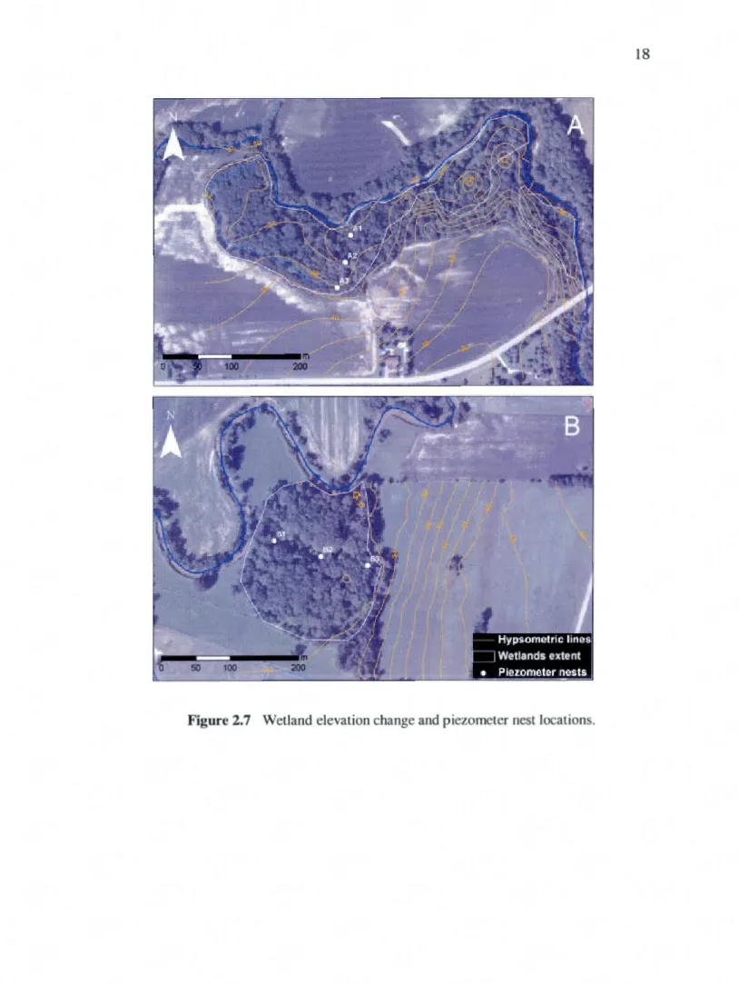
and b) wetland B ... 17 2.7 Wetland elevation change and piezometer nest locations ... 18 2.8 Piezometer nest transects ... 19 2.9 DTS cable installed near wetland A (from July 9 to 16, 2012) and wetland B

(from July 29 to August 1, 2012) ... 21 3.1 Revised Quaternary deposits map ... 26 3.2 Hydraulic conductivity (K) in a) Wetland A, b) Wetland B. The photograph

shows the type of fine sediments that were present at the piezometer where K was not measurable ... 27 3.3 The "freedom spa ce" of the de la Roche River near a) wetland A and b)

wetland B. Both wetlands are part of the freedom space based both on flood space (blue zone) and mobility space (M2 grey diagonals), which represents mobility related to the meander characteristics (Ml zones represent mobility

3.4 Longitudinal profile of the Rock River study area ... 29 3.5 Changes in water levels (elevation above sea levet) in the river (black tine)

and in the piezometers from April to October 2012 for A) wetland A and B)

wetland B (see Figure 2.7 for piezometer locations) ... 30 3.6 Rain and discharge (at the CEHQ gauging station) for four precipitation

events in 2012: a) July 23 (59 mm), b) September S (61 mm), c) October 6

(27 mm) and d) Oct ob er 19 (35 mm) ... 31 3.7 Change in water levels (elevations above sea levet) in the river and in the

piezometers for both wetlands to rain events occurring on a) July 23 b) September 5, c) October 6 and d) October 19 (see Figure 3.5). Note that the elevation in wetland A (located upstream) is always higher than in wetland B

(downstream) ... 32 3.8 Cross-correlation between the levet in the river and the levet in the three

piezometers for wetlands A and B in 2012 ... 34 3.9 Cross-correlation between Philipsburg precipitation and the water levels in

the river and in the piezometers of the two wetlands ... 35 3.10 Water temperature in the piezometers in both wetlands ... 36 3.11 Change in air temperature (green) and water temperature in the river at

wetland A (blue) and B (red) for the events of a) July 23, b) September 5, c) October 6 and d) October 19. The flood hydrograph is shown in gray (dashed tine) as a guide to locate the peak discharge (discharge values do not

correspond to the values on the y-axis) ... 37 3.13 Changes in water temperature in the river from May to October 2012 A) from

upstream to T05 and B) from T06 to wetland B. The air temperature is shown in gray (gray dashed line) ... 39 3.14 Spatial variation of the maximum temperature measured by the DTS A)

wetland A and B) wet B. Note that the temperature scale is not the same in

both cases ... .40 3.1 S Average and maximum temperatures measured using the DTS at both

wetlands ... 41 3.16 Standard deviation of the measured temperatures using the DTS at both

wetlands ... 41 3.17 Maximum temperature data obtained from DTS measurements from Figure

3.1 S for a) wetland A and b) wetland B, here presented using the sa me col our Jegend ... 42 3.18 Stable water isotope samples analyzed from the River Rock ... .43

3.19 Radon concentration variability along the Rock River during the sampling

conducted in the mon th of August 20 12 ... .44 3.20 Measured and simulated total discharge and 222Rn activity ... .45

Dans le contexte de la gestion intégrée des bassins versants, les milieux humides riverains peuvent jouer un rôle important dans le corridor fluvial (aussi appelé espace de liberté). Les milieux humides riverains peuvent surtout contribuer à la normalisation des interactions nappe-rivière et dans une certaine mesure aider à atténuer les effets des pressions anthropiques et des changements climatiques. Cependant, les connaissances sur la connectivité aquifère-rivière sont très limitées dans le sud du Québec et il est très difficile de quantifier les fonctions hydrologiques des milieux humides riverains dans les conditions actuelles. L'objectif de ce projet était d'améliorer la compréhension de la connectivité entre la rivière de la Roche située en Montérégie, deux milieux humides situés à l'intérieur de l'espace de liberté de cette rivière, et l'aquifère. Pour déterminer si ces milieux humides riverains jouent un rôle important dans la dynamique de la rivière, ceux-ci ont été instrumentés pour surveiller les niveaux et les températures de l'eau à l'aide de sondes Hobo et d'un Distributed Temperature Sensor. Les chroniques ainsi mesurées ont été traitées au moyen d'analyses corrélatoires. Les échanges nappe-rivière ont également été mesurés au moyen de l'analyse de l'activité 222Rn. Les deux milieux humides riverains présentaient de nombreuses similitudes en termes de taille, de végétation et de leur proximité au cours d'eau. Toutefois, des différences significatives ont été observées en ce qui a trait aux fluctuations des niveaux d'eau entre la nappe phréatique et la rivière. Le milieu humide A est relié de façon plus dynamique à l'aquifère comparé au milieu humide B où les sédiments sont plus fins et les conductivités hydrauliques sont plus faibles. Les différences hydrogéomorphologiques jouent probablement un rôle dans la réponse hydrologique distincte des deux milieux humides, car le milieu humide A est situé dans une ancienne boucle de méandre du chenal, et Je milieu humide B est situé là où Je lit de la rivière est resté dans la même position pendant au moins les 83 dernières années. En outre, les apports d'eau souterraine à la rivière sont apparemment diffus pour la majorité de la zone d'étude, à J'exception d'une contribution locale d'eau souterraine immédiatement en amont du milieu humide B révélée par les données de température de J'eau et de l'activité du radon. Toutefois, cette contribution de l'aquifère située proche de la zone humide B ne peut pas être directement liée à la présence du milieu humide étant donné le comportement très différent des deux

milieux humides relativement similaires à bien des égards. Cette variabilité marquée observée entre les deux milieux humides étudiés suggère que la prudence est requise lorsque l'on regroupe ensemble tous les milieux humides riverains. Leur impact hydrologique peut être plus variable que prévu dans la plupart des systèmes de gestion de rivière.

MOTS-CLÉS : milieux humide nveram, connectivité nappe-rivière, espace de liberté, hydrogéomorphologie, distributed temperature sensor, radon.

In the context of integrated watershed management, riparian wetlands can play an important role within the river corridor (also called freedom space). In particular, riparian wetlands can contribute to the regulation of aquifer-river interactions and to sorne extent help mitigate the effects of anthropogenic pressures and climate change. However, knowledge about aquifer-river connectivity is very limited in southern Quebec and it is currently almost impossible to quantify the hydrological functions of riparian wetlands in today's conditions. The objective of this project was to increase the understanding of interactions between the Rock river in the Montérégie region, two wetlands located within the freedom space of this river, and the aquifer. To determine whether these riparian wetlands played an important role in control ling river dynamics, they were instrumented to monitor water levels and temperatures using Hobo sensors and a Distributed Temperature Sensor. The time series were subsequently analyzed using cross-correlation analyses. Interactions between the river and wetlands were also assessed through measurements of 222Rn activity. The two riparian wetlands exhibited many similarities in terms of size, vegetation and proximity to the channel. However, significant differences were noted in the relationship between water table and river channel levels fluctuations. Wetland A is more dynamically connected to the aquifer than wetland B where sediments are finer and hydraulic conductivities lower. Differences 111 hydrogeomorphology probably play a role in the distinct hydrological response at these two wetlands, as wetland A is located in a former meander loop of the channel, and wetland B is located where the river channel has remained in the same position for at !east 83 years. In addition, groundwater inflow to the river is apparent! y diffuse over most of the study area with the exception of a local groundwater contribution immediately upstream of wetland B, which was evident from both water temperature data and radon activity. However, this aquifer contribution in the surrounding wetland B cannot be directly linked to the presence of the wetland given the very different behavior of the two relatively similar wetlands in most respects. This marked observed variability between the two studied wetlands suggests that caution is required when grouping ali riparian wetlands together. Their hydrological impact may be more variable than assumed in most river management schemes.

KEYWORDS: riparian wetland, aquifer-river interactions, nver corridor, hydrogeomorphology, distributed temperature sensor, radon.

INTRODUCTION

1.1 Context

Sustainable and integrated management of rivers entails severa! issues related to the quantity and quality of water, the prevention of water damage to homes and infrastructure, the possible Joss of agriculturalland and forest from bank erosion, the conservation of biodiversity in rivers and in the riparian zone and finally the use of the water resource for recreation and recreational tourism. Ali these issues must contribute to the sustainable management of river systems by taking into account the fluvial dynamics and its response to environmental changes. Indeed, whether they are undisturbed or severely destabilized by frequent anthropogenic interventions (e.g. changes in land use, changes in a river's course, dredging), river systems remain both sensitive across the flow section and resilient at the scale of a homogeneous reach. This dynamic balance between rivers and the many related issues is intrinsically linked to the need to adapt the current management of rivers to climate change, because the variations in temperature and especially in the intensity, duration and volume of rainfall, could have a major impact on rivers in the coming decades.

Wetlands can play an important role in the regulation of aquifer-river interactions and could to sorne extent help mitigate the effects of anthropogenic pressures and climate change. However, knowledge about aquifer-river connectivity is very limited in southern Quebec and it is currently al most impossible to quantify the hydrological functions of riparian wetlands in today's conditions. It is even more difficult to estimate how these functions could help mitigate the effects of anthropogenic pressures and climate change.

1 .2. 1 Groundwater-surface water interactions along ri vers corridors

Integrated watershed management is increasingly recognizing that rivers are not a linear entitity in space, but that by integrating their temporal dynamics, they occupy a larger space, often called a corridor. A river corridor represents a complex system of land, plants, animais and streams that is not yet weil understood. Within the broader context of the "Freedom space" research project, of which this project is a sub-component, the river corridor is defined as the flooding space and the mobility space required by a river to function nominally. A river corridor is an integrated management framework based on the hydrogeomorphology of rivers. 1t is a relatively new concept, not yet implemented in Quebec, but which is gaining popularity in different parts of the world (Parish Geomorphic, 2004; Piégay et al., 2005; Kline and Cahoon, 2010). A river corridor approach aims to identify the flooding and mobility spaces required by the river and allows it to evolve in these areas rather than forcing it to move in a way that is shaped by human interventions. This framework appears to be much more promising for sustainable management in a changing climate, because it helps maintain the natural physical features of rivers (transporting water and sediment) and thus increases their resilience.

A natural river has a complex and diverse flora and fauna habitat compared to a straightened river: alternating between fast sections and slower, deeper sections (pools), a varied granulometry and heterogeneous banks. Therefore, improved flood mitigation also results in the improvement of the ecological functions of streams and their biodiversity, and of the ir ecological goods and services (Kline and Cahoon, 201 0). In addition, a river corridor recognizes the importance of connectivity between the river and the aquifer, notably through wetlands which can contribute to flood mitigation (Bullock and Acreman, 2003; Piégay et al., 2005; Arnaud-Fassetta et al., 2009), !essen the severity of low flows, as weil as filter underground contaminants and provide healthy ecosystems.

Aquifer-river interactions in the presence of wetlands may be highly variable in ti me and space (Krause et al., 2007; Baskaran et al., 2009) and are influenced by a variety of factors (e.g. topography, geology, river discharge). In humid climates, rivers can receive a significant contribution of groundwater for a large part of the year (Hayashi and Rosenberry, 2002; Hayashi and van der Kamp, 2009). The hydrological modeling completed by Lavigne et al.

3

(20 1 0) for example showed that the contribution of groundwater discharge to the Châteauguay River can reach 66% of the total river discharge. However, there are few of these studies in Quebec where the size of the fluxes exchanged between surface and grou nd water flows, their location and the local processes involved in these interactions are little known. The areas where groundwater discharges into the river can alternate with areas where the river feeds the aquifer (Datry et al., 2008). These interactions take place in the hyporheic zone, an intermediate zone between the river sediments and the underlying geological materials, where different types of water mixes from different sources. This zone is influenced by heterogeneities in the sediment hydraulic conductivity distribution and the topography of the streambed (Woessner, 2000). Channel morphologie features can also interact with changes in stream stage and lateral groundwater inputs in ways that can substantially influence the a mount of hyporheic ex change flow (HEF) over time, across seasons or within a single storm event. At low stage, the water surface more closely follows streambed topography that creates steeper head gradients that support more HEF (Wondzell and Gooseff, 2013). The hyporheic zone also pla ys an important role in the transfer of pollutants and of heat fluxes, and is an important component of the riparian ecosystem (Brunke and Ganser, 1997; Alexander et al., 2002). ln general, groundwater is cooler than surface water in the sumrner months and during periods of low flow it is expected that groundwater inflow to the river might be detected via a cooler temperature signature near the riverbed.

1.2.2 Wetlands

According to article 1.1 of the Ramsar Convention, wetlands are defined as "areas of marsh, fen, peatland or water, whether natural or artificial, permanent or temporary, with water that is static or flowing, fresh, brackish or salt, including areas of marine water the depth of which at low tide does not exceed six metres" (Ramsar Convention Secretariat, 2006). This is clearly a very broad definition, and severa! classifications are used to distinguish the different types of wetlands in terms of vegetation, slope, groundwater and surface water connection. A simple classification is that ofKeddy (201 0), which distinguishes four types: swamps, marshes, bogs and fens. This type of classification is main! y based on vegetation. The Cowardin wetland classification system (Cowardin et al. 1979), on the other hand, combines hydrology and vegetation characteristics to define five categories, namely riverine, lacustrine, palustrine,

marine, and estuarine (the latter being associated with saltwater and/or coastal waterbodies). In Canada, the usual classification system is that of Warner and Rubec (1997) which has one more class than the Keddy (2010) classification, namely swamps, marshes, bogs, fens and shallow water. Finally, the hydrogeomorphic classification (HGM) aims at classifying wetlands based on a clarification of the relationship between on three components: geomorphic setting (topographie location within the surrounding landscape), water source (precipitation, surface/near surface flow, groundwater discharge) and hydrodynamics (direction and strength of flow (hydrologie head)) (Brinson, 1993). Originally, there were four wetland classes in the HGM approach, namely depressional, extensive peatland, riverine and fringe wetlands. These were later developed into seven classes, i.e. riverine, depressional, slope, mineral soil flats, organic soit flats, estuarine fringe, lacustrine fringe (Smith et al. 1995).

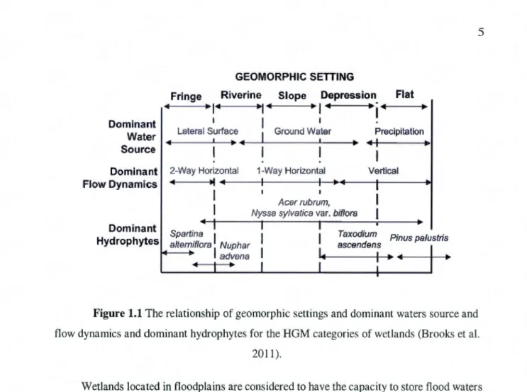
It is clearly difficult to determine which classification approach is best to cover the wide range of wetland types in given areas. For example, Brooks et al. (20 Il) use a combination of the HGM and National Wetland Inventory (NWI) to determine classes for the Mid-Atlantic Region in the U.S.A. The approach relies Jess on vegetation than the NWI since similar species composition can be observed in very different geomorphic contexts and flow dynamics (Figure 1.1, Brooks et al. 20 Il). In this revised classification scheme, se ven classes are used: marine tidal fringe, estuarine tidal fringe, flats, slope wetlands, depressions, lacustrine fringe and riverine wetlands. Figure 1.1 shows that the geomorphic setting has a clear influence on the dominant water source to the wetland.

Dominant Water Source Dominant Flow Dynamics Dominant GEOMORPHIC SETTING

Slope Depression Flat Fringe Riverine

..

"'1..

..1

1 Lateral Surface 1 1 .. ..

i .,.

__

____..,

1 2-Way Horizontal

Ground Water Precipitation .. 1

1-Way Horizontal Vertical

..

.. 111!'4---t---f-~---t---+1

1 1

Acer rubrum, Nyssa sylvatica var. biflora Spartina

l

Hydrophytes alterniflora Nuphar 1 advena

Taxodium Pinus palustris ascendens

Figure 1.1 The relationship of geomorphic settings and dominant waters source and flow dynamics and dominant hydrophytes for the HGM categories of wetlands (Brooks et al.

2011).

Wetlands located in floodplains are considered to have the capacity to store flood waters and thus effective! y reduce or delay the risk associated with flood peaks (Bullock and Acreman, 2003; Piégay et al., 2005; Barnaud and Fustec, 2007; Hudson et al., 20 12). This buffering keeps flood waters in the wetland for a white and releases them in the dry period, contributing to the maintenance of river flows during the driest times of the year (Dennison and Berry, 1993; Barnaud and Fustec, 2007; Mitsch and Gosselink 2007; Morley et al., 20 Il). This contribution is even more important in the case of wetlands connected to groundwater. Several studies show that between 30 and 70% of water supplied to rivers may come from groundwater discharge through wetlands (Warwick and Hill, 1988; Cole et al., 1997; Uchida et al., 2003; Krause et al., 2007. Morley et al., 2011 ;. Bourgault et al., 2014).

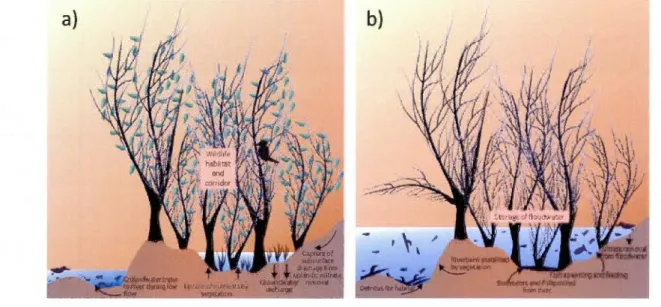
Riparian wetlands are known to play severa) ecosystem serv1ces (Figure 1.2). In agricultural watersheds, they are particularly effective at reducing nitrate reaching strearns (Zedler, 2003). It is now recognized that the oxygen-starved Gulf dead zone (approximately 15,000 km2, NOAA, 2013) is directly connected to the tost ecosystem services provided by wetlands in the states of Illinois, Iowa, Minnesota, Wisconsin, Indiana, Ohio, Illinois, and Iowa

have removed over 85% of the wetlands (Zedler, 2003). lncreasingly, restoring wetlands in agricultural watersheds is seen as one of the solutions to the problem. However, this requires a sound understanding of their hydrological and ecological roles. For example, large wetlands can support many bird species (Mensing et al., 1998) and smaller wetlands can host rare plants (Zedler, 2003). Upstream wetlands play a minor role in trapping nutrients, whereas downstream wetlands in sorne agricultural watersheds can remove up to 80% of nitrates (Crumpton et al. 1993). lt is thus very important to better understand riparian wetland processes to prioritize those which would need protection or restoration of ecosystem services such as biodiversity support, nutrient removal and flood reduction.

Figure 1.2 lllustration of severa! potential ecosystem values for riparian wetlands

during a) dry season and b) flood season (from Mitsch and Gosselink, 2007)

Hydrological connectivity of riparian wetlands is particularly important since it may

affect their potential for nitrogen removal via denitrification (Racchetti et al., 2011; Roley et al. 20 12). Aquatic and wetland biodiversity are a Iso often related to hydrological connectivity (Phillips, 2013). Connectivity is often assessed using map elevation and water levels in the river, but it is also strongly related to abandoned channel water bodies such as meander loops (Phillips, 2013). As such, it is a dynamic concept which can evolve over time following geomorphic evolution of the river channel (Amoros and Bomette, 2002; Phillips, 2013). New

oxbow lakes tend to vary in stage in a similar way to the river channel, whereas older oxbow

lakes, even if located very close to the channel, can be essentially isolated from it, at least in

terms of surface water (Hudson, 201 0). Overall, channel-floodplain connectivity is complex

and cannot simply be determined by variables such as distance from channel and differences

in elevation between the channel and the wetlands (Phillips, 20 13). In sorne cases, flow into floodplain depressions can occur even if flow stage in the channel is below bankfull, with

impacts on both cross-and down-valley fluxes (Phillips, 2008).

There is a Jack of understanding of hydrological connectivity between riparian

wetlands formed through meander eut-off, mainly because most studies of hydrologie

connectivity use a simple discharge threshold approach instead of an analysis of the actual

water levet data to assess connectivity (Hudson et al. 2012). Wetlands that are located within

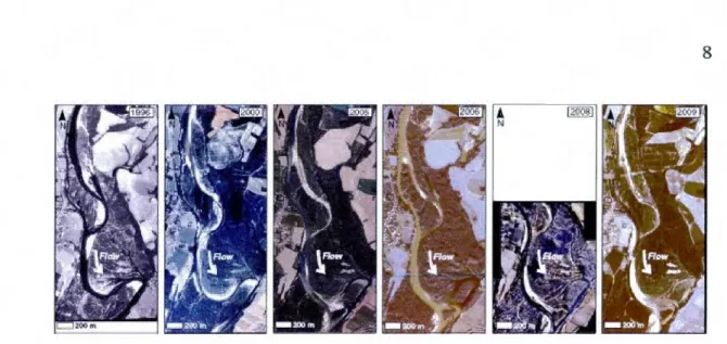
a river corridor ("freedom spa ce") are intrinsically related to hydrogeormorphologica 1 processes of meander dynamics. Because of lateral migration and resulting chute cutoff in meanders (Hooke, 1995; Zinger et al. 2011), meander oxbows are formed. Four evolutionary stages of geomorphic adjustment normally follow meander cutoff, which are known as the "oxbow lake cycle" (Gagliano and Howard, 1984). The first stage is the intial cutoff wheras the final stage consists of the near complete sedimentary infilling of the oxbow lake, which remains as an arc ua te wetland (Hudson et al., 20 12). A good illustration of this process is provided by a recent cutoff in the Ain River, in France (Dieras et al., 20 13). A large wetland is

now occupying the former course of the channel after the cutoff which occurred between 2000

Figure 1.3 Aerial photographs showing the Ain River (France) between 1996 and 2009. A riverine wetland was formed after the cutoff of the meander loop in the bottom right

part of the photos (Dieras et al. 20 13).

A better assessment of hydrologie connectivity of the HGM-defined nvenne (or riparian) wetlands, is needed for integrated floodplain management, particularly in the context of climate change (European Commission, 2009). It is also essential to understand the variability of hydrologie connectivity in riverine wetlands within the river corridor, as wetlands in these zones may have been created by different processes (e.g. meander cutoff, beaver dam construction), and they may be at different geomorphological stages of evolution (Cabezas et al. 2011 ). The first stage of evolution is the initial cutoff whereas the final stage consists of the near complete sedimentary infilling of the oxbow lake, which remains as an arcuate wetland (Hudson et al. 20 12). As shown in Figure 1.1, the dominant water source in these types of wetlands should be a combination of lateral source and groundwater, with mainly a one-way horizontal flow dynamic.

1.3 Objectives and methodology

Given its importance in the hydrological dynamics of rivers, a better understanding of

the river-water connectivity and the contribution of riverine or riparian wetlands to this connectivity is fundamental in improving the management of floodplains and streams. The

objective of this research is to better understand interactions between a river, wetlands and the

aquifer and hence reinforce the beneficiai hydrological functions of the river corridor. To atta in

agricultural river in southern Quebec, where two riparian wetlands are studied. The river corridor ("freedom space") of the Rock River has been recently characterized by Biron et al. (20 13). This analysis revealed that one of the wetlands is created following a meander cutoff that occurred between 1930 and 1964, whereas the other wetland is located in a zone where the river channel has not moved in the last 83 years.

To determine whether these riparian wetlands play an important role in control ling river dynamics such as flooding (in the vertical plane) and meandering (in the horizontal plane), they were instrumented to monitor water levels and temperature. These data were cross-correlated and analyzed at different timescales. A distributed temperature sensor was utilized in the river adjacent each wetland to measure the water temperature and look for signs of groundwater recharge. Surface and groundwater samples were collected for 180, 2H and 222Rn analysis. A Quaternary deposit survey was performed to validate the existing map, soil samples were collected for granulometry analyses and slug tests were done to determine hydraulic conductivity.

This thesis is divided in four chapters. The Introduction presents the general context, followed by a description of the state of the knowledge in river-aquifer-wetland interactions. Chapter II presents the methods used in this research, wh ile Chapter III describes and discusses results. The Conclusion summarizes the results and brings sorne opening thoughts that go beyond this research.

This project is a part of the larger "Freedom space" project that was funded by the Ouranos consortium (PACC-26 program). Partial results were presented during the "Earth, Wind and Water -Elements ofLife" CWRA-CGU conference in Banff, Alberta from June 5-8,2012.

METHODOLOGY

2.1 Study area

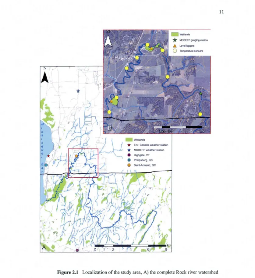
The Rock River is located in the Montérégie region, 80 km southeast of Montreal. The Rock River watershed drains a surface area of approximately 145 km2, of which 55 km2 is Quebec territory. The 27 km long river flows northward from its source in Vermont to Saint-Armand in Quebec, and southward from there toits mouth Missisquoi Bay in Vermont (Figure 2.1A). The study area is limited to the 9 km river section located in Quebec. In this section, the tributaries Brandy, Swennen and au Ménés enter the Rock River (Figure 2.1 B).

The watershed land use is predominantly agriculture (41 %), particularly m the downstream sector, and forest (40%) (Hegman et al., 1999; MAPAQ, 2002). Residential land is uncommon (5.4%) and commerciaVindustrialland is nearly non-existent. The profound loss of sediment and nutrient storage functions at a watershed scale due to channelization, drainage works, and flood plain encroachments, has resulted in an increase in fluvial erosion hazards such as flood and erosion damage, and an upward trend in sediment, soit, and nutrient exports (V ANR, 2009).

s

q u

*

Wetlands

Env Canada weather station MDDEFP weather stat1on H1ghgate, VT

Ph1lipsburg. OC Sa1nt-Armand, QC

Figure 2.1 Localization of the study area, A) the complete Rock river watershed

2.1.1 Climate

Daily temperature and precipitation measurements are available from the Philipsburg Environment Canada weather station, located approximately 3 km west of Saint-Armand. Houri y precipitation measurements are available from the Philipsburg weather station, located approximately 7 km north of Saint-Armand (Figure 2.1A). The climate of the region is characterized by moderate temperatures, a sub-humid volume of precipitations and a long growing season. The climate normals for the period 1971-2000 indicate an average daily temperature of 6.8°C and total annual precipitations of 1096 mm (Environment Canada, 20 13).

2.1.2 Geology

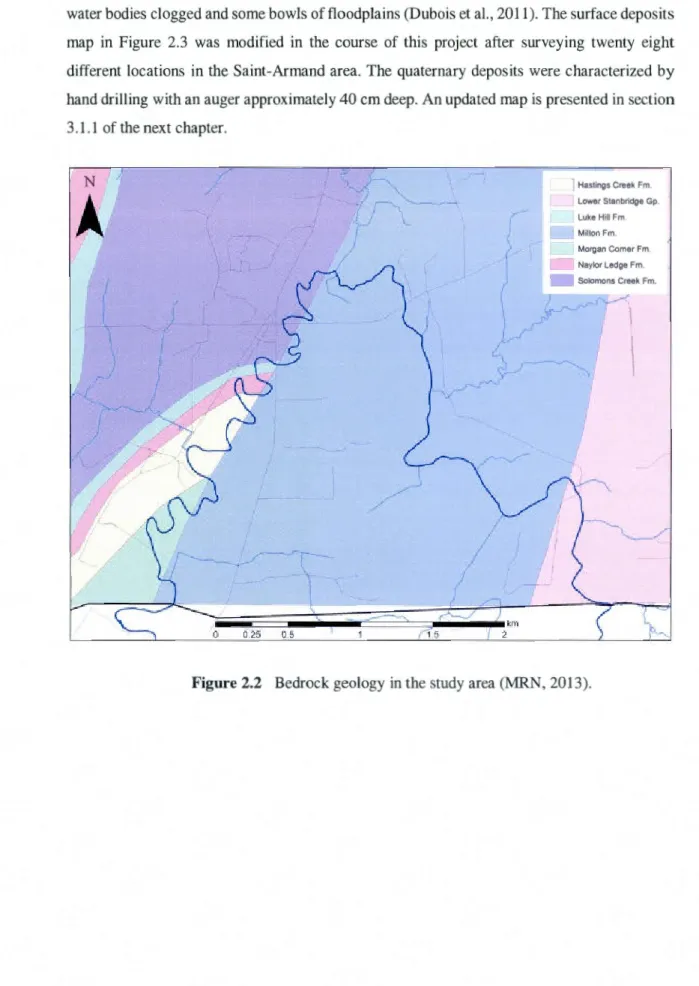
The Rock River watershed geology is composed of shale and slate-fractured shale, and to a lesser extent dolomite, sandstone and limestone (Dennis, 1964; Stewart, 1974; Mehrtens and Dorsey, 1987). The bedrock geology (Figure 2.2) largely determines the topography of the watershed. The terrain along the Champlain fault directs the watershed drainage towards the north, to Quebec. Severa! outcrops also influence the position and profile of the channel.

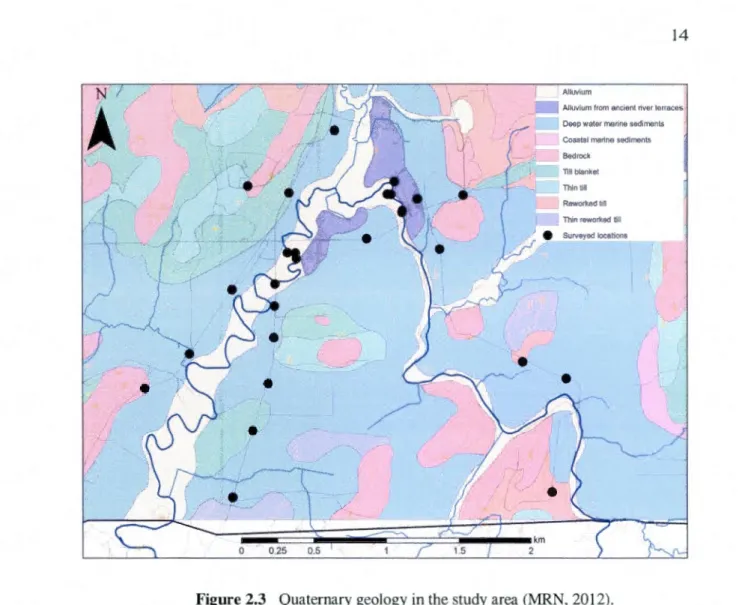
The Rock River is located at the boundary of two physiographic units, the St. Lawrence Lowlands and the Appalachian Plateau. The first outcrops belonging to the Plateau appear as elongated ridges that dominate the lowest few meters of land, as seen in the towns of Philipsburg and Saint-Armand (Dubois et al., 2011). The surface deposits of the area consist primarily of deep-water marine sediments (MGa), till blanket (Tc), thin till (Tm), reworked till (Tr) and many sections of extruded rock at the peaks of nearby hills. The river itself rests on alluvium (Ap) and there are few areas of alluvium from ancient river tenaces (At) due to minimal meandering of the river over the past century (Figure 2.3). Till covers much of the watershed due to its glacial history. The fine, silty and clayey glaciolacustrine deposits mask the till underneath, which resulted from the presence of glacial and proglacial lakes during the deglaciation that began about 13,000 years BP (Dubois et al., 2011 ). There are also marine sediments reflecting the intrusion of the Champlain Sea about 12800 to 10200 years BP (Stewart and McClintock, 1969; Cronin, 1977). The downstream portion of the Rock River flows mainly on marine sediments (Figure 2.3). The river is also much more sinuous than in the upstream portion where it flows directly on till or on the bedrock. Organic deposits are of limited extent, and are usually found in forested depressions in the land, ancient and isolated

water bodies clogged and sorne bowls of floodplains (Dubois et al., 20 Il). The surface deposits

map in Figure 2.3 was modified in the course of this project after surveying twenty eight different locations in the Saint-Armand area. The quaternary deposits were characterized by

hand drilling with an auger approximately 40 cm deep. An updated map is presented in section

3.1.1 of the next chapter.

r

\ 0 0~25 0.5 Hastings Creek Fm. Lower Stanbridge Gp. Luke Hill Fm. Milton Fm Morgan Corner Fm Naylor Ledge Fm.

(

\

1

•

Alluvium from ancient river le!Taces

Deep water manne sediments Coastal manne sediments

e ./

0 0.25

Figure 2.3 Quaternary geology in the study area (MRN, 2012).

According to the Missisquoi Bay watershed portrait (Dubois et al., 20 Il), a crescent of orthic and humic gleysols with few intrusions of podzols are present along the northeastern boundaries of the watershed. The central part of the watershed is dominated by brunisolic order soils (clay loam to sandy loam). To the north of the watershed, there are also dystric order soils such as humo-ferric, orthic, and gleyed podzols.

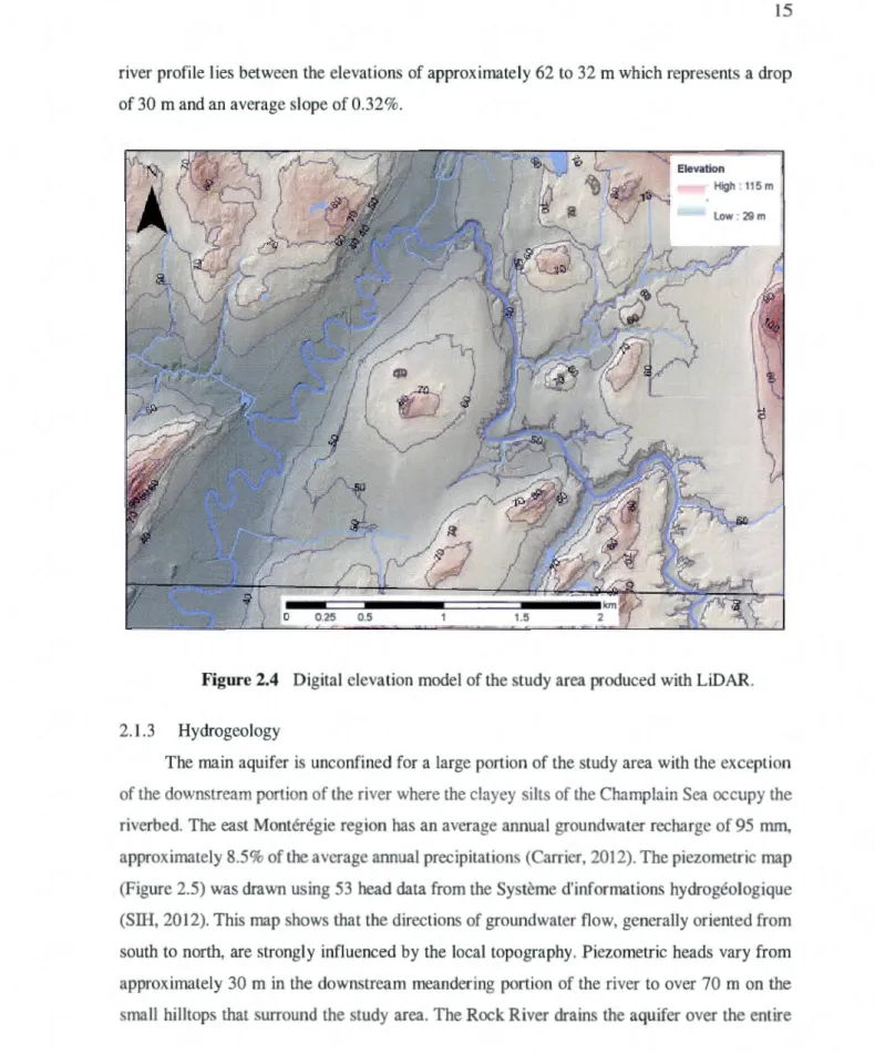
Figure 2.4 shows the topography of the study a rea and was produced with high resolution LiDAR measurements. The upstream portion of the river is visibly more incised than the downstream portion. The highest elevations in the Rock River watershed are approximately 260 rn and are located in the upper reaches of the watershed in Vermont. Elevations are in the order of 30 rn near the mouth of the Missisquoi Bay. The Quebec portion of the longitudinal

river profile lies between the elevations of approximately 62 to 32 rn which represents a drop

of 30 rn and an average slope of 0.32%.

Figure 2.4 Digital elevation madel of the study area produced with LiDAR.

2.1.3 Hydrogeology

The main aquifer is unconfined for a large portion of the study area with the exception

of the downstream portion of the river where the clayey silts of the Champlain Sea occupy the

riverbed. The east Montérégie region has an average annual groundwater recharge of 95 mm,

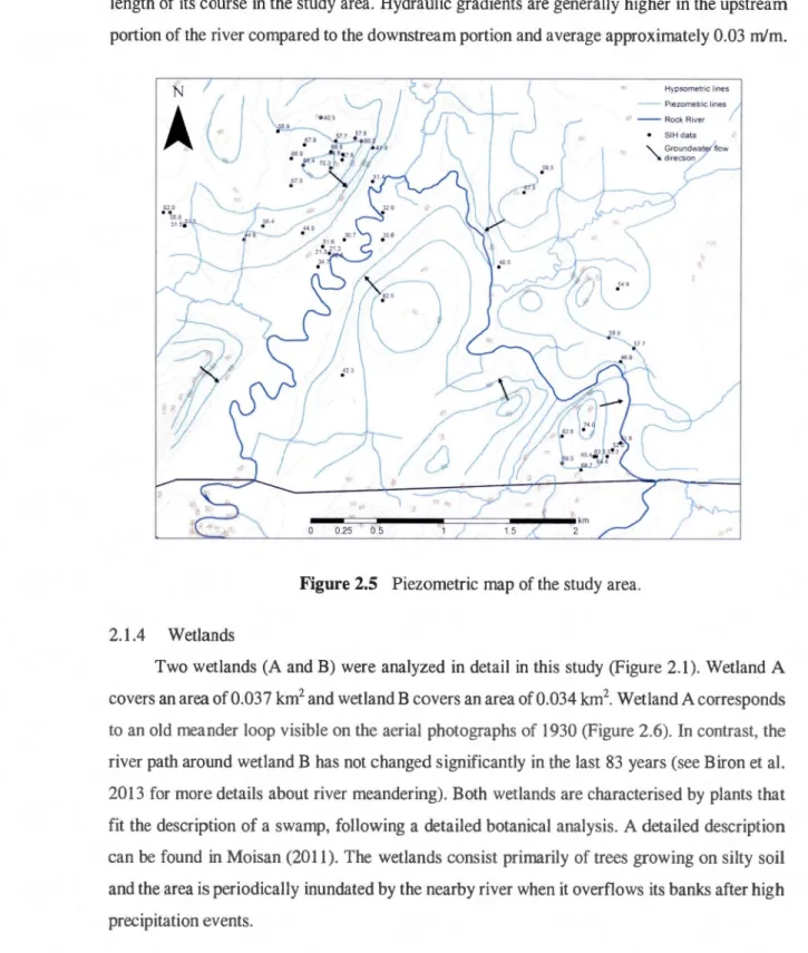
approximately 8.5% of the average annual precipitations (Carrier, 2012). The piezometrie map

(Figure 2.5) was drawn using 53 head data from the Système d'informations hydrogéologique

(SIH, 2012). This map shows that the directions of groundwater flow, generally oriented from south to north, are strongly influenced by the local topography. Piezometrie heads vary from

approximately 30 rn in the downstream meandering portion of the river to over 70 rn on the

1ength of its course in the study area. Hydraulic gradients are generally higher in the upstream portion of the river compared to the downstream portion and average approximately 0.03 ml m.

À

(J

2.1.4 Wetlands

0.25 0~5 1 )

Hypsometrie lines - Piezometrie lmes

Figure 2.5 Piezometrie map of the study area.

Two wetlands (A and B) were analyzed in detail in this study (Figure 2.1 ). Wetland A

covers an area of0.037 km2 and wetland B covers an area of0.034 km2. Wetland A corresponds

to an old meander loop visible on the aerial photographs of 1930 (Figure 2.6). In contrast, the river path around wetland B has not changed significantly in the last 83 years (see Biron et al. 2013 for more details about river meandering). Both wetlands are characterised by plants that fit the description of a swamp, following a detailed botanical analysis. A detailed description can be found in Moisan (2011). The wetlands consist primarily of trees growing on silty soi! and the area is periodically inundated by the nearby river when it overflows its banks after high

Figure 2.6 Evolution of the de la Roche River between 1930 and 2009 at a) wetland

A, and b) wetland B.

2.2 Instrumentation

2.2.1 Piezometer profiles in wetlands A and B

In June 2011, three piezometers nests were hand drilled with an auger along a transect perpendicular to the river within each wetland (Figure 2.7). Each transect position and

elevation was accurately determined via differentiai global positioning system (DGPS, Trimble

R8GNN) to produce a digital elevation madel of each wetland. Wetland A topography has

values ranging from 33 to 43 m. Wetland B is more flat with an elevation of about 31 m throughout the entire area. The piezometrie transects have a length of 1 J 0 and J 90 rn for

wetland A and B, respective! y. The piezometers have a diameter of 2.54 cm, and a totallength

of 3.45 rn and 4.95 rn respective! y with a screened casing of 0.30 m. The depth of the shallow and deep piezometer in each nest was 3.15 and 4.65 rn, respectively (Figure 2.8). From

November 201 J to October 2012, Solinst (LTC Levelogger Junior) pressure transducers were placed within each of the shallower piezometers to measure the water table levet every 15 min.

Ali time-series were corrected for atmospheric pressure with data produced from a Solinst

18

Levellogger A 30 ,. +---~r----.----~---~--~r-_J~---~~~---.---.----. ·10 10 20

,,

B

33 32 31 :§: 30 •• g iS 29 LB 27 26 25 ·20 20 40 30 40 50 60 80 60 Distance (m) 100 120 Oistilnce (ml 70 80 90 100 140 160 IBO

Figure 2.8 Piezometer nest transects.

llO 120 130

2.2.2 Temperature sensors in the river

In June 20 Il, eight Hobo sensors that measure temperature every 15 min were installed on the riverbed over the total river length (Figure 2.1 B). Six sens ors were recovered in September 2011. In May 2012, eight sensors were re-installed in the same locations and six were recovered in November 2012. The other sensors could not be retrieved from the river sediments and were considered !ost. The Solinst sensors installed in the piezometers and in the

river (see below) also recorded temperature every 15 minutes (see Figure 2.1 B for sens or local ization).

In the summer of 2012, a fine-resolution spatial and temporal analysis on the temperature

variability in the wetlands was performed usmg a DTS

(Agi lent Distributed Temperature Sensor, N4386A). This 1.5 km fibre optic cable was installed in the river for severa! days and measured the temperature at every meter every 15 minutes (Figure 2.9). Wetland A measurements were recorded from July 9 to 16, and wetland B measurements were recorded from July 29 to August 1. The maximum air temperature during

these two periods was 30°C and did not vary significantly during the sampling period. GPS points were recorded at regular intervals to georeference the DTS and analyze the spatial

variability of the temperature. The vegetation cover and depth of the river were also

georeferenced to determine the cause of the detected cooler zones (shaded area, greater depth,

Figure 2.9 DTS cable installed near wetland A (from J uly 9 to 16, 20 12) and wetland B (from July 29 to August 1, 20 12).

2.2.3 Water levels and discharge measurements

A custom tubing setup was installed in the river adjacent to each wetland transect. Within each tube, a Solinst pressure transducer was installed to measure the water leve! of the river

ev er y 15 min. Water levels were measured between June 20 Il and October 2012 near wetland

B, and from June 2012 to October 2012 near wetland A. The exact position of the Solinst

sensor was obtained with a DGPS. Ali time-series were corrected for barometric pressure from

the Solinst Barologger.

A gauging station operated by the Centre d'Expertise Hydrique du Québec (CEHQ)

measures discharge every 15 minutes since 2001 upstream of the two wetlands (station 030425;

(CEHQ, 2013). However, there have been discharge peaks of more than 35 m3/s registered during the June 2011 to October 2012 study period. Discharge was also measured six times adjacent to each wetland (see Figure 2.1 B, locations LLA and LLB) during the summer 2012

using an acoustic Doppler velocimeter (ADV, Nortek Vectrino).

2.3 Water sampling

2.3.1 Stable isotopes in water

Thirty-two water samples were collected for the analysis of stable isotopes in water

C

80

and 2H) in July 2011. The samples were sealed in 30 mL polyethylene botties devoid of air and preserved at 4°C in the refrigerator to prevent contamination and evaporation until analysis.

Fifteen samples were taken directly from the river, 12 directly from the piezometers, four from the oxbow lakes, and one from the municipal weil. The piezometers were purged in advance to ensure the sampled water had minimal contact with the atmosphere. The analyses were completed in February 2012 using mass spectrometer in the GEOTOP Laboratory at UQAM. The results of the analysis were corrected with a calibration curve that was constructed with three reference materials normalized on the VSMOW-SLAP scale.

2.3.2 Radon

Radon-222 is a radioactive isotope with a short half-life of 3.8 da ys. It is produced from the decay of Radium, 226Ra, in ali rocks. It accumulates in liquid form in confined and se mi-confined aquifers, however once released it quickly degasses to the atmosphere. It is therefore expected that groundwater would have higher concentrations of 222Rn than surface water. Thirty-two samples were collected for analysis in August 2012 during a period of low flow in the river (Q

=

0.02 m3/s). Fourteen samples were taken directly from the Rock River, three

from its tributaries, nine from households that are sourced by wells, and six from the wetland piezometers. The piezometers were purged in advance to ensure the sampled water had minimal contact with the atmosphere. The direct method of analysis was used for these samples

because they did not contain the necessary volume of water to use the extraction method. A

3.0 mL sample was collected with a syringe and inserted into 4.5 mL of Maxilight Hidex

scintillation liquid contained in a 10 mL glass vial. The rest of the samples were collected in 250 mL glass botties devoid of air to be analyzed with the extraction method in the laboratory.

Radon-222 was analyzed using a Hidex (LS 300) liquid scintillometer at UQAM using the

protocol developed by Lefebvre et al. (20 13 ).

2.4 In situ tests

2.4.1 Slug tests

A slug test is an in situ permeability test. In August 2012, two rounds of tests were completed in the shallower of the two piezometers in each nest. The pressure transducers were

set to record water levels every second and approximately !50 mL of water was added to the piezometer to effect a hydraulic head change of approximately 30 cm. The rate at which the water leve! returned to its initial hydraulic head allowed the calculation of the hydraulic

conductivity (K) using the Hvorslev method (Hvorslev, 1951 ).

2.4.2 Granulometry

Eight soi! samples were collected by hand drilling with an auger to a maximum depth of 3.40 m near each piezometer nest. The samples were analyzed in the !ab by soaking them in

water, to prevent pilling of fine clay partiel es, and filtering with meshes ranging from >2 mm

to <38 11m to determine the sediment classification. Clay is defined as particle sizes between 0 and 2 11 m, fine silt between 2 and 20 11 m, silt between 20 and 50 11 m, fine sand between 50 and 200 11 rn and sand between 200 Il m and 2 mm (Clément and Pelta in, 1 998).

2.5 Modelling and temporal analyses 2.5.1 Radinl4

Radinl4 is an Excel mode! that calculates the rates of groundwater inflow to streams from environmental tracers (Cook et al., 2008). In the current research, running the mode!

required values for radon activity and electrical conductivity which were measured in different locations over the total length of the river, at the entrance of three tributaries into the main river and also in severa! bedrock wells. The river width, depth and discharge are also required along the entire length of the study area. Groundwater inflow to the river over the total river length is calibrated to reproduce measured discharge. The gas transfer velocity which describes the rate of Joss of radon to the atmosphere through the water surface was calibrated to reproduce measured 222Rn activities.

24

Water leve! fluctuations in the river and in the piezometers were analyzed graphically

through cross-correlation and autocorrelation analyses performed with the software PAST

(Hammer et al., 2001). This type of analysis provides information on the causal relationship

between the input and output time series, and can thus be used to determine the influence of

one series on the other based on the lag time between the two series and on the intensity of the

correlation. These analyses were used to determine the leve! of correlation and the time lag

between 1) precipitation in the area and water levels in both the river and piezometers, 2)

fluctuations of water leve! in the river and the piezometers, and 3) air temperature and water

RESULTS AND DISCUSSION

3.1 Geology and hydrogeology

3 .1.1 Quaternary deposits and granulometry

The revised Quaternary deposits map (Figure 3.1) correct! y constrains the river within

the alluvium deposits, particularly in the downstream portion of the river. The bedrock

coverage was extended to the west of the upstream portion of the river and on the hill to the

northwest of Saint-Armand. An area of till blanket was added and another was extended in the

central part of the map and an area of reworked till was enlarged north of the upstream portion

of the river. Severa! other minor modifications were made based on the surveyed Quaternary deposits. Both wetlands are located in the area of alluvium surrounding the Rock River.

In wetland B, 46% of the analyzed particles are silt to fine silt (<38 !Jm) and 39% are in the range of 63 to 500 !Jffi categorized as fine to coarse sand. There are no particles larger than 500 !Jm. In wetland A, 43% of the analyzed particles are fine to coarse sand (63 to 500 Il rn)

and only 16% are silt to fine silt ( <38 Il rn). There are lesser percentages of particles in ali other

categories up to >2 mm. The sediment compositions in both wetlands appear to be divided

between fine sand and fine silt, but in wetland B, the mix is skewed towards fine silt resulting

in lower hydraulic conductivity (section 3.1.2) and a groundwater response (section 3.2) that

1)J

A

Alluvium from ancient river terraces

1

(

_

)

\

J

)

1

/

0 0.25

Figure 3.1 Revised Quaternary deposits map. 3.1.2 Hydraulic conductivity

Wetland B is characterized by finer sediments than wetland A, and hydraulic conductivity (K) varies from being non measurable to 5.7xl0·7

mis, whereas K varies between

5.3xl0-7

and 4xl0-6 _mis

in wetland A (Figure 3.2). As a comparison, sediments with hydraulic conductivities ranging from 1 to 10-3 mis are usually considered to be permeable (typically weil sorted gravel and/or sand) whereas K values from 10-4 to 10·7 mis represent semi-permeable material (very fine sand, silt, loess or loam, peat, or layered clay). For hydraulic conductivities ranging from 1

o-

8 to 1

o

-

'

2 mis, sediments are considered impervious to water (Bear, 1972).

Thus, wetland A falls in the semi-permeable category, wh ile wetland B falls on the low end of semi-permeable and also in the impervious category.

The interactions between surface and groundwater are severely impaired in wetland B

with such low hydraulic conductivity values. In wetland B, the aquifer cannot reduce the impact

of flooding significantly by absorbing ex cess surface water during a flood and slowly releasing

it afterwards. Signs of flooding such as high water mark on vegetation and matted vegetation

are commonly observed in wetland B after large precipitation events. In wetland A, the aquifer

buffers the impact of floods more effectively with a hydraulic conductivity one order of magnitude greater than in wetland B.

Figure 3.2 Hydraulic conductivity (K) in a) Wetland A, b) Wetland B. The photograph shows the type of fine sediments that were present at the piezometer where K was

not measurable.

3.1.3 Geology, wetlands localization and the river corridor

Both wetlands exhibit very similar vegetation, are of similar size and are located m depressions close to the channel. Thus, regardless of the classification scheme that would be used, they would be considered of the same type. However, slug tests revealed marked differences in hydraulic conductivity, which willlikely affect hydrologie connectivity. In terms of river corridor management and integrated floodplain management framework, these two wetlands may therefore play a different role. The fact that wetland A was in the very recent

past strongly connected to the channel, prior to the cutoff which occurred sometime between

1930 and 1964, should also be taken into account in the analysis. In any case, the two wetlands are part of the "freedom space" which was determ ined by Biron et al. (20 13) on the de la Roche

River (Figure 3.3). In the current study, it is possible that wetland B also originated from meander migration with the river corridor, but it would be at a later stage of development of the oxbow lake cycle (Gagliano and Howard, 1984).

Figure 3.3 The "freedom space" of the de la Roche River near a) wetland A and b) wetland B. Both wetlands are part of the freedom space based both on flood space (blue

zone) and mobility space (M2 grey diagonals), which represents mobility related to the

meander characteristics (Ml zones represent mobility based on computed lateral migration rate) (Biron et al. 2013).

Figure 3.4 shows the longitudinal profile of the river from upstream to downstream. Wetland A is located adjacent the river from approximately 4000 to 5500 m while wetland B is approximately 8000 to 8700 rn downstream. There is a slope difference in the river along these two locations which visibly affects the sediment size on the riverbed. At approximately

4000 rn, the majority of the riverbed consists of rocks approximately 5 to 30 cm in diameter

mixed with finer sediment. Reading towards 5000 m downstream where the piezometers are

located and where granulometry samples were collected, the riverbed sediment gradually turns

to coarse sand. By 5500 rn downstream, the riverbed is mostly fine sand and silt and remains

as such for the remainder of the study area. The differences in sediment size within each

wetland could be explained by this change in river slope resulting in coarser sediment being

deposited in wetland A and finer sediment in wetland B when flooding over the river bank

occurs.

55 50

e

- ; 45 .Q

_...

~ 40 ..!!! w 35 30 0 1000 2000 3000 4000 5000 6000 7000 8000 9000 10000

Distance from upstream (rn)

Figure 3.4 Longitudinal profile of the Rock River study a rea.

3.2 Water levels

3.2.1 Seasonal scale

Figure 3.5 presents data from April to October 2012. lt should be noted that the levels

in the river adjacent to wetland A were estimated from the measured values adjacent to wetland

B bef ore June 21, wh en the Solinst pressure transducer was installed (grey dashed li ne on

Figure 3.5a). lt is clear from Figure 3.5 that the water table fluctuates synchronously with the

river levels near wetland A, especially for the two piezometers clos est to the river (Al S and

A2S; see Figure 2.8 for the position of piezometers). Starting in July, major rainfall events

create a temporary increase in the leve! of the river beyond the elevation of the piezometers

AIS and A2S. The momentary reversai ofhydraulic gradients is also observed for two major

events in the fall (September 5 and October 6). ln wetland B, the aquifer response to changes

in the river water leve! is much lower. The groundwater levels gradually decline throughout

the summer of2012 until the 61 mm precipitation event on September 5, which causes a sudden

increase in river water level, with arise of 1.5 rn for piezometer B3S. For this event and for the

26 mm precipitation event on October 6, levels in the river temporarily exceed the levels in the

three piezometers. These results indicate that the river is more dynamically connected to the

34.5 A) - AIS 31.5 B) - BtS 34.0 - A25 A3S 31.0 33.5 Ê

I

_30.5 ~33.0 :J :J

"'

"'

~ 32.5 Q) > 30.0

z

z

32.0 29.5 31.5 31.0 29.0 N N N N N N N N N N N N N N N ~ N N N N N N ~ ~ ~ ~ 8 _~ 8 _~ ~ ~ ~ ~ ~ ~ ~ s ~ s ~ ~ ~ ~ ~ ~ 0 _~ 0 0 _~ N N

s

~ ~ % ~ ~ ~ v. v. ;;;- ;::- ;::- ~ 0;- 0;- _~ ;;- v. ;::- 0;- 0;- è> 0 0 ~ 0 0 0 0 0 0 0 _~

~

~ _~ 0 0 0 0 0 0

§

;::; _::;: ;::; _{~ ~} è> _~ ~ Oo _{~ ~ ~ ~ ~} Oo _~ 0 "' "' 0 N 0 ~ 0

Figure 3.5 Changes in water levels (elevation above sea leve!) in the river (black li ne) and in the piezorneters from April to October 2012 for A) wetland A and B) wetland B

(see Figure 2.7 for piezorneter locations). 3.2.2 Precipitation events scale

Four precipitation events were analyzed in more detail in 2012: July 23 (59 mm ofrain), September 5 (61 mm of rain), October 6 (27 mm of rain) and October 19 (35 mm of rain) (Figure 3.6). The heavy rain in July did not result in a significant flood event (peak discharge of about 2 rn3/s), whereas the early September event, nearly identical in terms of total prescipitation, generated a peak flood of over 16 rn3/s. The two events occurring in October resulted in sirnilar peak discharge values (1 0-11 m3/s).

a) 2.5 2.0 ~ _{m 1.5} .§. ~ :0 1.0

...

0 0.5 - Débit - Précipitation 2 Ë .§. "' c 0 'l' "' 5

-a

v 6 ~ 0.0 ~_J~----~~====~~==~--_JB 23/07/2012 25/07/2012 27/07/2012 29/07/2012 b) 18 .----16

"'

0 1 14 -;;; 12 ...

l

lO

~ 8 :0 - Débit

.

..

0 6 - Précipitation o +-~~--~~~~~~--~---~-+ 04/09/2012 08/09/2012 12/09/2012 16/09/2012 c) 12 ,_-,....---..., 10 - Débit - Précipitation 0 +---~~--~---r--~--~--~--~~--~---+ 04/10/2012 08/10/2012 12/10/2012 d)u -r--- ""' 0 10 - Débit ~ :0

.

..

0 4 - Précipitation

o

t::=::::::~~--~--

-.----~

--====----t

8

0 2 Ë .§. c 0 4 'l ' !'l ël. 'ü ~ 6 0.. 18/10/2012 22/10/2012 26/10/2012

Figure 3.6 Rain and discharge (at the CEHQ gauging station) for four precipitation

events in 2012: a) July 23 (59 mm), b) September 5 (61 mm), c) October 6 (27 mm) and d) October 19 (35 mm).

The contrast in the response of the two wetlands is also apparent at the event scale

(Figure 3.7). In July, the precipitation of 59 mm had an impact, albeit small, on water levels in the three piezometers at wetland A (Figure 3.7a). However, the change in piezometers at wetland B was negligible. In September, the water leve! in the wetland A piezometers rises

very rapidly, by 1.5 rn in 15 hours for Al, and then decreases progressively (Figure 3.7b), while

the water leve! in the wetland B piezometers rises more gradually and continues to rise for

severa! days after the rain. There is also a cap on the water leve! in wetland B indicating a

spreading of the flood (hydrograph with shark fin shape, Figure 3.7b) in the swamp (this

behavior is not observed in wetland A). During both floods in October, the groundwater leve! remains nearly constant and at the same water leve! for the three wetland B piezometers, wh ile groundwater levels fluctua te with that of the river and are lower for the wetland A piezometers

that are closest to the river (Figure 3.7c,d). Note that the spreading of the flood (shark fin shape

hydrograph) is also observed for the October 6 event at wetland B (Figure 3.7c), although it is

not as pronounced as for the September 5 event.

23/07/2012 33 Ê

'i

32 ~ z 31 30 25/07/2012 27/07/2012 29/07/2012 29~~~~~~~~~~~-, 03/10/2012 07/10/2012 11/10/2012 15/10/2012 b) 34 33 Ê -; 32 " " > z 31 30 29~~~~~~~~~~~ 03/09/2012 07/09/2012 ll/09/2012 15/09/2012 d )34 33 Ê -; 32 " ~ z 31 30 17/10/2012 21/10/2012 25/10/2012

Figure 3.7 Change in water levels (elevations above sea leve!) in the river and in the

piezometers for both wetlands to rain events occurring on a) July 23 b) September 5, c) October 6 and d) October 19 (see Figure 3.5). Note that the elevation in wetland A (located

Water Jevels in wetlands A and B show highly contrasted responses to precipitation

events. This can be 1 inked to the geology of the surrounding areas and to the processes that led to their development. As mentioned above, wetland A has developed from an ancient meander.

This probably influences the fine hydrostratigraphy of the sediments in this area and could

exp lain its more important hydraulic connectivity. In contrast, welland B has developed on fine sediments. It reacts slowly to precipitation events and to high river flows, but appears to store

more water as a temporary surface reservoir. 3.2.3 Cross-correlation analyses

The contrast in the hydrological connectivity between wetlands also appears clearly in the cross-correlation analysis (Figure 3.8). For wetland A, the correlation is very high (from 0.90 for piezometer Al to 0.77 for piezometer A3) and the time Iag between the peak in the

river and in the piezometers is Jow (6 to 21 hours). The maximum correlation for wetland B is

0.61, with lag times more than an order of magnitude higher, up to 330 hours (Figure 3.8). The

gap is shorter in wetland A, which is explained by the coarser sediments that facilitate the

transfer of the pressure wave in the riparian zone. It is expected that the !ag time between the

level in the river and the level in the piezometers increase as the distance between the river and a given piezometer increases, however this is not exactly the case given the granulometry of

the sediments, as weil as perhaps the position of the piezometers relative to hydrostratigraphic

pathways that may be present in the sediments of each wetland.

The correlations between rain events and groundwater levels (Figure 3.9) are much lower than the correlations between river water levels and groundwater levels (Figure 3.8).

This is explained by a significant transformation of the rain signal as it passes through the unsaturated zone. This was also highlighted by the two precipitation events of similar magnitude (July 23 and September 5, 20 12) which resulted in very different responses of the water table (Figure 3.7a,b). The maximum correlations between rain events and groundwater

levels are of the same order of magnitude for the two wetlands (maximum of 0.09 for wetland A and 0.05 for wetland B).

In wetland A, the time lag between river levels and groundwater levels is similar to the Jag between therain events and the river level, and shorter than the Jag between therain events

and the groundwater levels. This indicates that in this wetland, the river levet actually has an effect on the groundwater levels. The asymmetric shape of the cross-correlation between river levels and groundwater levels confirms that the primary function plays a direct role on the second (in the case where the two functions are simultaneously and independently influenced by precipitation, cross-correlation is symmetrical). In wetland B, the gap between the rain

signal and the groundwater levet is shorter than that between the river levet and the groundwater levet. It is therefore not possible to conclude that variations in the river levet cause variations in the groundwater levet.

Figure 3.8 Cross-correlation between the levet in the river and the levet in the three

Figure 3.9 Cross-correlation between Philipsburg precipitation and the water levels

in the river and in the piezometers of the two wetlands.

The pattern of cross-correlation observed at wetland A exhibits similarities with results

from Cloutier (20 13) on a riverine wetland in the Matane River (Gaspésie) with much coarser

grain size, and thus much larger hydraulic conductivity values. As the Matane wetland is also

located in a former meander loop, it seems to indicate that the geomorphic process which

created the wetland, or the evolutionary stage it is at, considerably affects the hydrological

response. In other words, riparian wetlands with a fairly wide array of sediment size can behave

in a similar way if their hydrogeomorphological evolution is similar. Or perhaps this indicates

that a certain threshold is reached between fine sand and clay, where hydrologie connectivity

varies. Since grain size and hydrogeomorphological processes are closely correlated, it may in

fact not be possible to distinguish them.

3.3 Water temperature

The study of water temperature dynamics is essential to properly characterize

hydrological connectivity (Poole and Berman, 2001; Poole et al., 2008; Cabezas et al. 2011 ).

The combination of continuous water leve! and temperature data measurements in this study

hyporheic water input is expected to dampen daily fluctuations in temperature in the channel and, in sorne cases to also modify the mean temperature (Cabezas et al. 2011).

3.3.1 Temperature changes in the wetland

Groundwater temperature in the three piezometers in both wetlands vary little over the course of a year, with a minimum of approximately 5°C generally occu1Ting in April and a maximum between 13°C and l4°C at the beginning of October (Figure 3.1 0). Observed variations follow those of the air temperature during the year, without a marked change in relation to rainfall events (this was confrrmed via cross-correlation analyses, not shown here). Groundwater temperature in the piezometers is therefore influenced by long-term variations in air temperature and is not under the influence of variations in the river leve!. This is contrary to what was observed by Cloutier (20 13) on the Matane River where groundwater levels in the piezometers within 50 rn of the river carried the influence of water levels in the river. This difference could be explained by the coarser sediments and higher hydraulic conductivities in the Matane River.

14 13 12 6 5 4 +----.----~---,----,----,----~---,----~---,----~---,----. 11/2011 12/2011 12/2011 01/2012 02/2012 03/2012 04/2012 05/2012 06/2012 07/2012 08/2012 09/2012 10/2012

Figure 3.10 Water temperature in the piezometers in both wetlands.

At the event scale, there are marked differences in trends of river temperature between wetlands A and B following the passage of the July 23 and September 5 flood (Figure 3.11 a,b ).

ln contrast, the river temperature is almost identical for the two floods in October (Figure 3.llc,d). ln July, the river temperature at wetland A follows very closely the air temperature