Robust Relay Beamforming for MIMO Multi-Relay Networks with Imperfect Channel Estimation
Texte intégral
Figure
Documents relatifs
in [7]: they consider multiple clusters of users that wish to exchange messages locally within each cluster, with the help of a single relay.. Achievable rates for DF, CF, AF and
The closed-form expressions for the optimal tuning of the AR(2) parameters and mean square error (MSE) performance have been first established as a function of the second and
demonstrates that due to the proposed training approach, unlike the existing channel estimators for AF relaying networks, e.g., [10], channel estimation performance of the
In particular, it is shown that, by properly choosing the network code, the equivalent code can show Unequal Error Protection (UEP) properties, which might be useful for
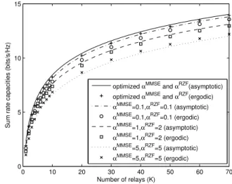
The end-to-end instantaneous mutual information in the asymptotic regime is derived in Section III, while the singular vectors of the optimal precoding matrices are obtained in
It is assumed that the source node is unaware of the specific channel controlling the communication but knows the set of all possible relay channels.. Since the relay and
[6] H. Le-Ngoc, “Diversity analysis of relay selection schemes for two-way wireless relay networks,” Wireless Personal Communications., vol. Song, “Relay selection for two-way
Next, given the advantages of the free probability (FP) theory with comparison to other known techniques in the area of large random matrix theory, we pursue a large limit analysis
