Towards Probabilistic Timing Analysis for SDFGs on Tile Based Heterogeneous MPSoCs

HAL Id: hal-02305048

https://hal.archives-ouvertes.fr/hal-02305048

Submitted on 17 Jan 2020

HAL is a multi-disciplinary open access

archive for the deposit and dissemination of

sci-entific research documents, whether they are

pub-lished or not. The documents may come from

teaching and research institutions in France or

abroad, or from public or private research centers.

L’archive ouverte pluridisciplinaire HAL, est

destinée au dépôt et à la diffusion de documents

scientifiques de niveau recherche, publiés ou non,

émanant des établissements d’enseignement et de

recherche français ou étrangers, des laboratoires

publics ou privés.

Towards Probabilistic Timing Analysis for SDFGs on

Tile Based Heterogeneous MPSoCs

Ralf Stemmer, Hai-Dang Vu, Kim Grüttner, Sébastien Le Nours, Wolfgang

Nebel, Sébastien Pillement

To cite this version:

Ralf Stemmer, Hai-Dang Vu, Kim Grüttner, Sébastien Le Nours, Wolfgang Nebel, et al.. Towards

Probabilistic Timing Analysis for SDFGs on Tile Based Heterogeneous MPSoCs. 10th European

Congress on Embedded Real Time Software and Systems (ERTS 2020), Jan 2020, Toulouse, France.

#paper 59. �hal-02305048�

Towards Probabilistic Timing Analysis for SDFGs

on Tile Based Heterogeneous MPSoCs

Ralf Stemmer

, Hai-Dang Vu

, Kim Gr¨uttner

,

Sebastien Le Nours

, Wolfgang Nebel

and Sebastien Pillement

†_{University of Nantes, France, Email: {hai-dang.vu, sebastien.le-nours, sebastien.pillement}@univ-nantes.fr} ‡_{OFFIS e.V., Germany, Email: kim.gruettner@offis.de}

Abstract—Performance and timing prediction of complex par-allel data flow applications on multi-core systems is still a very difficult discipline. The reason for it comes from the complexity of the hardware platforms with difficult or hard to predict timing properties and the rising complexity of the software itself. In this work, we are proposing the combination of timing measurement and statistical simulation models for probabilistic timing and performance prediction of Synchronous Data Flow (SDF) applications on tile-based MPSoCs. We compare our work against mathematical and traditional simulation based performance prediction models.

We have shown that the accuracy and execution time of our simulation can be suitable for design space exploration.

Index Terms—Probabilistic SystemC Model, Multi Processor, Real-Time Analysis

I. INTRODUCTION

Today’s and even more future life will be assisted by many small computer systems for sensing and interaction with its environment. The evolution towards the Internet-of-Things era is nowadays challenged by providing high data and sensing quality which will be assisted through machine learning and other AI techniques. Connected with this change is the major challenge of partitioning software between the node (edge, fog) and the cloud. Because of the growing demand in computational efficiency at the edge and fog level, more and more embedded systems are designed on multi-core platforms. In this context, our work addresses the challenge of perfor-mance prediction and optimization of complex data processing software running on multi-core edge and fog platforms. On the one hand performance prediction with a high fidelity for one specific data flow mapping and implementation is very important for the validation of extra-functional requirements, such as timing. On the other hand a complete analysis of all possible mappings and implementations of a data flow application have to be quantitatively assessed for choosing the optimal mapping (w.r.t. timing constraints such as application end-to-end latency). In this work we focus on the design space exploration (DSE) aspect of performance analysis.

Performance and timing analysis of parallel software, run-ning on complex multi-core platforms is hard. In the domain of timing analysis of multi-core systems, existing simulation-based approaches and formal mathematical methods are deal-ing with either scalability problems for a large problem size or provide too pessimistic and thus unusable analysis results. Our work aims at improving scalability of analysis approaches by adopting probabilistic models and simulation techniques. The

result is an experimental framework to validate and improve statistical analysis techniques for data flow applications on tile-base multi-core systems. A tile tile-based MPSoC consists of mul-tiple processors with private instruction and data memory. Inter tile communication is realized via dedicated FIFO channels or shared memory. In a previous publication [1] we have already presented our measurement-based characterization approach and a SystemC based statistical simulation for probabilistic timing and performance analysis.

In this paper, we present the adoption of this approach to different case-studies. We systematically evaluate the benefits and limitations of our statistical simulation for timing analysis of two different data flow applications on tile based multi-core systems. For this reason, we have built an experimental setup for the comparison of our probabilistic modeling and analysis against measurements on a hardware prototype, a state-of-the-art static analysis and a simulation based approach. This setup is used for different case-studies and mapping configurations. Configurations are representatives of multi-core systems with dedicated FIFO channels, shared buses and shared memories. The evaluation metrics are accuracy of the estimations and analysis time. Moreover, scalability of the analysis approaches is evaluated with respect to different use-case, different platform configurations and different mappings. The paper is organized as follows: In the next section we are analyzing the state-of-the-art where we are positioning and comparing our approach against other works in the area of timing analysis for multi-core-systems. Sec III presents our approach and provides more details about the creation and structure of our proposed probabilistic simulation model. In Sec IV we present our use-cases, the experimental setup, our comparison results and finally a discussion of these results. The paper closes with a summary and outlook on future work.

II. RELATEDWORK

Analysis approaches are commonly classified as simulation-based approaches, which partially test system properties simulation-based on a limited set of stimuli, formal approaches, which statically check system properties in an exhaustive way, and hybrid approaches, which combine simulation-based and formal ap-proaches. Simulation-based approaches require extensive ar-chitecture analysis under various possible working scenarios but the created architecture models can hardly be exhaus-tively simulated. Due to insufficient corner case coverage, simulation-based approaches are thus limited to determine

guaranteed limits about system properties. Different formal approaches have been proposed to analyze multi-core systems and provide hard real-time and performance bounds. These formal approaches are commonly classified as state-based ap-proachesand analytical approaches. Despite their advantages of being scalable, analytical methods abstract from state-based modus operandi of the system under analysis which leads to pessimistic over-approximated results compared to state-based methods [2]. State-based methods are based on the fact of representing the system under analysis as a transition system and since they reflect the real operation states of the actual system behavior, tighter results can be obtained compared to analytical methods. Many recent approaches for the software timing analysis on many- and multi-core architectures are built on state-based analysis techniques [3]–[5]. However, state-based approaches allow exhaustive analysis of system properties at the expense of time-consuming modeling and analysis effort. The existing state-based approaches are thus dealing with scalability problems and multi-core architectures with complex levels of hierarchy in shared resources can hardly be addressed [5].

Statistical Model Checking (SMC) has been proposed as an alternative to formal approaches to avoid an exhaustive exploration of the state-space model [6]. As classical model checking approach, SMC is based on a formal semantic of systems that allows to reason on behavioral properties. SMC is used to answer qualitative questions1_{and quantitative} questions2_{. It simply requires an executable model of the} system that can be simulated and checked against state-based properties expressed in temporal logics. The observed executions are processed to decide with some confidence whether the system satisfies a given property. This allows systems that can not be assessed with an exhaustive approach to be approximated. Finally, as a simulation-based approach, it is less memory and time intensive than exhaustive state-based approaches. Various probabilistic model-checkers sup-port statistical model-checking, as for example UPPAAL-SMC [7], Prism [8], and Plasma-Lab [9]. SMC was adopted in [10] to evaluate a many-core architecture based on a 64-core homogeneous platform. The statistical model checking tool called BIP SMC [11] was used to evaluate the probability that timing aspects such as execution time and variability of processing time were bounded. The usage of UPPAAL-SMC to optimize task allocation and scheduling on multi-processor platform has been presented in [12]. Application tasks and processing elements were captured in a Network of Price Timed Automata (NPTA). It was considered that each task execution time follows a Gaussian distribution. In the scope of our work, we especially focus on the preparation process of probabilistic models of execution time. A comparison of formal model checking with SMC has been presented in [13]. A multi-processor system was modeled using timed automata and probabilistic timed automata in UPPAAL-SMC. While formal methods use only best and worst case execution times the SMC method allows to model the distribution of execution 1_{Is the probability for a model to satisfy a given property greater or equal} to a certain threshold?

2_{What is the probability for a model to satisfy a given property?}

Computation Time Model Communication Time Model Software Hardware

FPGA _{SystemC Model}Probabilistic Analysis_Results

Specifi-cation MeasurementInfrastructure MoC

MoA

Static Mathematical Model WCET SystemC Model

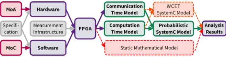
Fig. 1. Overview of our workflow. Hardware and Software gets designed following specific models. Then one instance of the system on an FPGA gets characterized. The resulting model can then be analyzed for real time properties (green). For evaluation we also create a static mathematical model shown with dashed red lines. And in dashed orange lines, only observed WCET gets considered.

times between those limits. The possibilities of modeling such a distribution is limited due to UPPAALs modeling language. In contrast to that work, our new SystemC approach allows to not only use a rough model of the distribution but the actual measured execution times. However, SMC methods have rarely been considered to analyze timing properties of applications mapped on multi-processor systems with complex hierarchy of shared resources, especially because the creation of trustful probabilistic SystemC models remains a challeng-ing task. Based on the established framework we attempt to systematically evaluate the benefits of using probabilistic SystemC models to analyze the timing properties of SDF based applications on multi-processor systems, targeting more tightness of estimated bounds and faster analysis times.

The novelty of our presented approach lies in the definition of a measurement-based modeling workflow for the creation of probabilistic SystemC models. SystemC models are calibrated with stochastic execution times that are inferred from mea-surement done on real prototypes with multi-processor archi-tectures. The efficiency of this workflow to architectures with different levels of complexity is evaluated through different case-studies.

III. APPROACH

Our established workflow is illustrated in Fig. 1. We show our input models for our approach in magenta. The computa-tion model is explained in detail in Sec III-B. The architecture model is explained in Sec III-A These models were used to design our hardware and software system. For later references, we highlighted assumptions with an A.

The system that gets build under the constraints of those models can then be analyzed regarding its timing behavior. Therefore we use a measurement infrastructure described in detail in [14]. This measurement method guarantees that there will be no interfering with the main system buses or non-predictable influence to the code execution on the processor.

The mapped and scheduled software gets executed on the designed hardware that gets instantiated on an FPGA. This real system is used to characterize the timing behavior of the hardware components as well as the actors of the SDF based application (shown in Fig. 1 in purple). Details about the measurement and characterization is presented in Sec III-C. The communication and computation time model get in-tegrated into a probabilistic SystemC model as shown in Fig. 1(green). The SystemC model is used for execution time

A0 A2 Read Write Actor-Execution FIFO Buffer Actor Channel Token Rate SDFG-Iteration A1 Tile 0 Tile 1 Shared Memory Private

Memory MemoryPrivate Mapping &

Scheduling

TMC Processing

Element ProcessingElement

Shared Interconnect Compute 1 1 2 1 A0 A1 A2 A2 A1 A2

Timing Measurement Infrastructure

TMU A2

A0

TMB

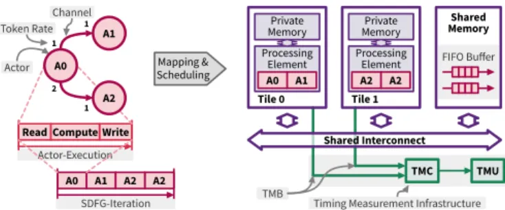
Fig. 2. Example of our MoC and MoA, showing a 3 Actor (Magenta) application mapped and scheduled on a 2 tile architecture (Purple). Additional the measurement infrastructure is shown (Teal).

analysis focusing on the distribution of the execution times. We also run a simulation only considering the WCET as comparison (Fig. 1 orange). Furthermore we apply a static mathematical model (Sec III-D), that considers the WCET of the actors and for communication (Fig. 1 red).

A. Model of Architecture

Our hardware platform follows the definition from [13] and [1]. A simple example of such a platform is shown in Fig. 2 (purple). In contrast to the referenced work, we scaled up the system to 7 heterogeneous tiles instead of only 2 tiles.

One processing element with a separate connected private memory is called tile. A1: Executing instructions from this private memory also causes no interference with other tiles. This allows us to design a composable multi processor system. In our system, some tiles are equipped with a floating point unit (FPU) or a hardware multiplier (MUL).

For data exchange between different tiles a shared memory is used, connected via a shared interconnect to the processors and A2: the arbiter uses Round-Robin strategy.

A3: For all memories we use static RAM an do not use any caches. The hardware gets instantiated on an FPGA. A4: All tiles and memories are connected to the same clock.

For comparison we also one experiment on a 4 tile system with peer-to-peer connections. The tiles are connected via exclusive hardware FIFO buffers. This hardware architecture is optimized for the communication structure of the application, so that communication can take part without any interference. B. Model of Computation (SDF)

We use Synchronous Data Flow (SDF) [15] as computation model (MoC). A simple example of an SDF graph is shown in Fig. 2 (magenta).

This model is used to describe the data flow between actors via communication channels . SDF offers a strict separation of computation (compute) and communication phases (read, write) of actors. During the compute phase, no interference with any other actor can occur. For MPSoCs this separation only works when the instructions are placed on separated memories (Assumption A1), connected with separate inter-connects to the processors as presented in Sec III-A. For communication, data get separated into tokens. It is assumed that A5: one token is exact one data word on the interconnect. Channels are FIFO buffers that can be mapped to any memory that is accessible by the producer (an actor that writes

on that channel) and the consumer (an actor that reads from that channel). During the read phase of an actor, tokens get read from the channels buffer. During the write phase, tokens get written into the channel. The amount of tokens a producer writes, or a consumer reads is called token rate. A6: The FIFO access is blocking. An actor can only switch to its compute phase after it read all tokens from all incoming channels. After the compute phase, the actor switches into write phase to write all tokens to the outgoing channels.

A7: The SDF application is self scheduled. After one actor finished writing onto all its outgoing channels, the next actor on the tile starts with its read phase. In case any depending actor (that gets executed on a different tile) did not write its token on the incoming channel of the scheduled actor, it polls on the buffers channel until the data is available.

C. Measurement

For our timing models we need to characterize the compute phase of actor as well as the communication between actors. For the compute phase we measure the amount of clock cycles a phase needs to be executed. This is done for different input data (input tokens). Since the code of an actor changes on different processors (e.g. with and without FPU), for each processor flavor this characterization needs to be done.

For the communication phases, we use a more sophisticated model that requires some static code analysis as described in [1]. Therefore the execution of instructions used to access a channel buffer gets considered as well. This allows us to simulate the communication in detail to know when and for how long communication takes place.

For measuring execution times we use a measurement infrastructure based on [14]. The infrastructure is split into three components. Two of them are shown in Fig. 2 (green).

The Time Measurement Unit (TMU) is basically a counter with the same cycle rate the processors have. The counter can be started and stopped from any tile individually without interference. When the counter got stopped, it sends its counter value via UART to a host computer. For this method, it is important that all components are clocked with the same fre-quency (Assumption A4). The management of the individual start/stop signals from the tiles are managed by the Timing Measurement Controller (TMC).

To connect each tile with the TMC a Timing Measurement infrastructure Bridge (TMB)is used to translate a data package from a peripheral bus into the individual control signals (start/stop). A8: We assume that each tile has independent communication features that do not interfere with the system bus (For example General Purpose Input/Output (GPIO) pins or a dedicated peripheral bus). This guarantees that starting or stopping a measurement does not cause any interference on the other bus systems. For our MicroBlaze based system, the AXI Stream Interfaces get used. Since the TMB is only a simple transcoder (if not directly GPIO pins are used), it is not explicitly shown between the tiles and the TMC in Fig. 2. From the measurements we not only get the BCET and WCET of specific parts of the software like the computation phase of an actor or the access of shared memory. We also get the distribution of execution times for the measured elements

which will be used in our probabilistic model. The BCET, WCET and average case execution time gets derived from the measured time values. In the context of our work, Worst- and Best-Case only describes the observed execution times. D. Static Analytical Model

This subsection presents the static analytical model we use to compare our simulation based approach with (See Fig. 1). For the static approach we need to make further assumptions that only relate to the static analytical model. We mark those assumptions with AS. The model is based on [16] and [17].

As mentioned in Sec III-B, the execution of an actor is split into three phases: read, compute, write. Those phases are also represented in the equation 1 for calculating the execution time of an actor. For the compute phase tcompute, the measured computation time of an actor gets used. The delay of reading tread(r) (Equ. 2) and writing twrite (Equ. 3) is a function of the token rate R(c) of a channel c. All incoming channels Cin and outgoing channels Cout need to be considered.

texec= X

c∈Cin

tread(r(c))+tcompute+ X

c∈Cout

twrite(r(c)) (1) The equations for reading (Equ. 2) and writing (Equ. 3) need to consider the bus access time for reading (tr) and writing (tw) data onto the bus. For our system, one token is one word on the bus (Assumption A5). Some computational

overhead needs to be considered via tc_r for the reading

procedure and tcw for the writing procedure. Bus arbitration

time ta is determined by Equ. 4. Those three delay parts

(tr/w, ta, tc) occur for each token r including further data rmeta for managing the FIFO buffer of a channel.

tread(r) = (rmeta+ r) · (ta+ tr+ tc_r) (2)

twrite(r) = (rmeta+ r) · (ta+ tw+ tcw) (3)

The arbitration delay ta (Equ. 4) is calculated under the assumption of having a Round-Robin bus arbiter (Assumption A2). Furthermore we assume for our static model that AS9: each other tile of all tiles (ntiles) of the system gets bus access before and that AS10: each of those tiles holds the bus access for the longest possible amount of time. For a single beat bus protocol this is ether reading or writing a word onto the bus.

ta= (ntiles− 1) · max (tr, tw) (4)

The data for the computation time of an actor (tcompute) comes from our measurement infrastructure (Sec III-C). The delay for tr/w as well. The computational overhead tc_r/w is based on static code analysis as presented in [1].

To calculate the time a complete iteration of executing the SDF application takes, the execution times texec for all actors that get executed in serial needs to be summed up. For actors that get executed in parallel, the longest execution time will be considered. Furthermore it is assumed that AS11: an actor gets only executed, when all its preceding depending actors are completely executed, which may take longer than waiting until all tokens on the channel are available.

Inter-connect Im pl em en ta tio n Tile 0 void Tile0::sc_thread(){ while(1){ ReadTokens(ChA);

wait(GetDelay(T_IDCTY));

WriteTokens(ChB); }} Shared Memory if(read) wait(t_r); else wait(tw); Si m ul at io n T0 Shared Memory T1 T2 Tile 2 Tile 1 while(1){ // Main loop

ReadTokens(&ChA, in); IDCT(in, out);

WriteTokens(&ChB, out); }

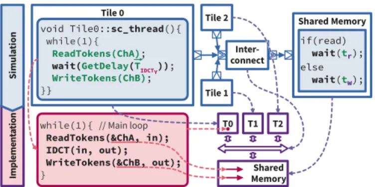
Fig. 3. Overview of our SystemC model with 3 tiles and how it is related to the later implementation of the simulated system. Tile 0 is presented in detail, with one actor (IDCTY) mapped on it.

For the peer-to-peer connected platform (Fig. 5, left) we can simplify some equations. The meta-tokens in Equ. 3 and Equ. 2 for managing the FIFO buffer are not needed because the FIFO behavior is implemented in hardware. Furthermore there is no arbitration. This leads to the following simplification: rmeta = 0, ta = 0. The value of tr/w as well tc_r/w must be adapted to the different implementation and bus interface. E. SystemC Model

The SystemC model is a representation of the whole system. It models the mapped and scheduled SDF application on a specific hardware platform. Fig. 3 shows in the top half the SystemC model for a 3 tile platform. In blue the parts of the SystemC model are shown, in green everything related to the measured timings (Sec III-C). The bottom half of the figure shows, how the simulated system gets transformed into the actual system. In purple hardware related parts are described, in magenta all software related parts.

The SystemC model consists of three major parts: 1) the Tile modules for simulating the actors’ execution on a tile, 2) the Interconnect module that simulates the bus behavior and 3) the Shared memory module for the read and write access to shared memory.

Tiles represent the actual tiles of the modeled platform as well as the execution of the SDF actors mapped on this tile. The timing behavior of the actors is simulated in an

SC THREADof the tile module. The computation phase of an

actor is a waitstatement using the actors’ computation time

tcompute ∈ ~Tactor. Furthermore the Tiles-Module provides a

model of the function used for communicating over channels. The timing behavior was analyzed and modeled in detail via static code analysis on instruction level we describe in [1].

The Interconnect module manages the structural integrity by connecting all tiles to shared memories.

The Shared Memory module simply distinguishes read tr and write access tw. Depending on the access type, it proceeds the simulation time by the related time.

In our simulation we use two representations of computation time. For WCET simulation the computation time of an actor is represented by its observed worst case computation time. For considering the distribution of execution times of an actor, we use all observed execution times. In each simulated

iteration of the system, a new execution time of an actor gets selected from a list of observed delays (see Fig. 3). This is realized by reading a text file that provides the raw measured computation time of this actor. We randomly select (using std::random_shuffle) data from the list of delays, taking care that no element of this list gets selected twice. We refer to this random selection of recorded execution times as injected data or injected distribution in the following experiments. Depending on the experiments it is possible to switch between Injected, Uniform or Gaussian distribution as well as only the WCET. For Uniform and Gaussian distribution we use the GNU Scientific Library(GSL) [18]. The parameters for these distributions are derived from the measured delays.

The Tile, Interconnect and Shared Memory SystemC mod-ules can be directly transferred to the real hardware. (Fig. 3) The target platform can be designed on an FPGA if the simulation not already represents existing hardware. The main loop of the SystemC threads represent the main loops of the firmware executed on the actual tiles. Instead of the wait-statement, the actual function of the actor must be called. Furthermore the ReadTokens and WriteTokens function now expect an address of a local buffer for the actual token.

To analyze different type of tiles with different processing elements, only the timing characteristics of the actors must be updated by measuring their computation time distribution on such a processing element. For different memories, the regard-ing access times, or the memory model needs to be updated. For different interconnects the ReadTokens and WriteTokens model as well as the interconnect module needs to be updated.

IV. EXPERIMENTS

This section describes our experiments. We first characterize all actors of our use-cases. Then we simulate different possible mappings to get the worst case and average case execution time, as well as a distribution of possible execution times of an iteration of the executed software. We then execute those experiments on the real platform and measure the actual execution times of each iteration to compare the real system’s behavior with our analysis.

We present our use-cases in Sec IV-A and our hardware platform in Sec IV-B. In Sec IV-C we describe the mapping of the use-cases on our platform. The characterization is shown in Sec IV-D At the end of this section we present and discuss the results of our experiments.

We provide git repositories3_{for our use-cases, measurement} infrastructure and models.

A. Use cases

In our experiments we want to analyze the execution time of an iteration of an SDF base application (Sec III-B). Therefore we apply our models to 2 different software applications:

Sobel-Filter (Fig. 4 left). In this use-case, the communica-tion part of the software takes most of the execucommunica-tion time. The computation part should be highly predictable when executed on tiles with an hardware multiplier, because there are only a few possible execution paths except of GetPixel actor. The

3_{Repository:https://gitlab.uni-oldenburg.de/stemmer/erts20} Get MCU IQY IQCr IQ_Cb IDCTY IDCTCr IDCT_Cb YCrCb RGB 64 64 64 64 64 64 64 64 64 64 64 64 64 64 64 64 64 64 3 3 3 81 81 81 81 1 1 1 1 Get Pixel ABS GX GY

Sobel-Filter JPEG Decoder

Fig. 4. Applications we use in our experiments represented as SDFG.

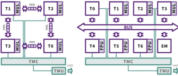
T0 FP U FP U FP U T4 M U L M U L M U L T1 T2 T3 M U L M U L T1 T2 M U L M U L T3 T0 FIFO FIFO FI FO _FIFO TMU TMC SM T6 T5 UART TMU TMC UART BUS

Fig. 5. We use a homogeneous platform with 4 peer-to-peer connected tiles (left) and a heterogeneous one with 7 tiles (right) connected via a shared interconnect. Some tiles have Floating Point Units (FPU) or hardware multiplier (MUL). In green the measurement infrastructure is shown with the Time Measurement Controller (TMC) that merges all control signals from the tiles to trigger the Time Measurement Unit (TMU).

results of analyzing this application could benefit from a detailed communication model as we use it in our simulation. JPEG Decoder (Fig. 4 right). This use-case has a huge computation part with an unmanageable amount of execution paths for most of the actors. Except for the inverse quantization (IQ-Actors) which is only a matrix multiplication and has only one execution path when a hardware multiplier is available. The results of analyzing this application would benefits from considering the distribution of possible execution times instead of just considering BCET and WCET.

B. Platform

For most of our experiments we use a heterogeneous mul-tiprocessor system with 7 tiles (Fig. 5 right). The individual tiles use a MicroBlaze soft core that is equipped with private memory. The tiles T1, T2, T3 are extended by a hardware multiplication unit (MUL). Tiles T4, T5, T6 are extended with a floating point unit (FPU). Furthermore there exists a shared memory that is used for communication between the tiles.

Since the Sobel-Filter use case has a high communication part compared relative to its computation part, we also built an experiment with a hardware platform that is ideal for this application (Fig. 5 left). It comes with 4 tiles that have a peer-to-peer connection to avoid any bus contention. These connections are realized by hardware FIFO buffers so that also the computational overhead for communication is reduced to a minimum to make analysis as simple as possible.

C. Experiment setup

This subsection describes the experiments we did with our use-cases. We label our experiments for later reference in the

results section. Furthermore we highlight and enumerate the hypotheses we want to check with an H.

For the Sobel-Filter we run 3 experiments: Sobel1,

So-belP2P and Sobel4. For the JPEG decoder we also run 3

experiments: JPEG1, JPEG3 and JPEG7.

For all experiments the instructions and local data of an actor is mapped on the private memory of a tile. The mapping of the actors of our application for the individual experiments is shown in Tab. I. With exception of the peer-to-peer ex-periment, all communication channels of our application are mapped on the shared memory of our platform (Fig. 5).

Sobel1 In our 1st experiment, we execute all actors of

the Sobel-Filter on a single tile that comes with a hardware multiplication unit. H1: This should be the most easy setup since the amount of possible execution paths are minimized and there is no contention possible on the interconnect.

SobelP2P In the 2nd _{experiment we run the Sobel-Filter}

on a 4 tile platform with peer-to-peer connection (Fig. 5 left). The mapping corresponds to the 4 tile mapping in Tab. I. H2: This setup shall avoid any bus contention, simplify the communication model by using hardware FIFOs and provide hardware multiplier to get a predictable multiprocessor system.

Sobel4 The 3rd _{Sobel-Filter experiment uses the same}

mapping as in the SobelP2P experiment, but now on the 7-Tile hardware platform (Fig. 5 right). Again, the mapping considers the usage of hardware multiplication.

These three Sobel-Filter experiments are used to evaluate the communication model of our simulation and static analysis model. Compared to the Sobel-Filter, the JPEG decoder is much more compute intensive and uses algorithms that come with much more execution paths.

JPEG1 In the 1st _{JPEG experiment we run all actors of}

the decoder on tile 0, that does not provide any hardware ac-celerators for multiplications and floating point operations. So these operations are done in software (via libgcc 8.2.0) which introduces further execution paths. H3: This mapping should lead to highly unpredictable execution times and challenge our probabilistic approach.

JPEG3 The 2nd JPEG experiment uses 3 tiles. H4: This

experiment should the execution paths since the actors benefit from the hardware accelerators they need.

JPEG7 In the last experiment all 7 tiles are used for

mapping the actors to focus on highest possible parallelisation. The actors are mapped on tiles that provide the hardware accelerators they can make use of. H5: This should lead to better predictable execution times for the computational part, but lead to much communication on the bus. This experiments challenges the communication model of our simulation and the static analytical model.

For the simulation using injected data we do 1 000 000 simulation runs, so that we make use of all observed timings. This is not an exhaustive simulation since this covers not all possible combination of execution times. For the WCET simulation we do only 10 000 runs, because the variety of input data is much less (one delay per actor).

D. Characterization

To estimate the execution time of an iteration of the exe-cuted application, the timing behavior for each actor needs to

TABLE I

MAPPING OF THESOBEL-FILTER ANDJPEGEXPERIMENTS ON THE TILES OF THE HARDWARE PLATFORM.

Experiment→ JPEG JPEG JPEG Exp. → Sobel Sobel Actor ↓ 1 Tile 3 Tile 7 Tile Actor ↓ 1 Tile 4 Tile

Get MCU 0 0 0 GetPixel 1 1

IQY 0 1 1 GX 1 2 IQCr 0 1 2 GY 1 3 IQCb 0 1 3 ABS 1 0 IDCTY 0 4 4 IDCTCr 0 4 5 IDCTCb 0 4 6 YCrCb RGB 0 0 0 be characterized once.

In our heterogeneous platform (Fig. 5) we have 3 different kinds of tile-based architectures. A simple MicroBlaze archi-tecture without any extension, an FPU extended MicroBlaze and a MicroBlaze with a hardware multiplication unit (MUL). Our two applications (Fig. 4) are compiled for all three architectures to make use of the additional instructions. The compilation process is only done once per architecture to make sure that the timing behavior of an actor never changes after it got characterized. The compiled actors then get only linked into the firmware of each processing element.

For measurement, a start and a stop instruction for the measurement infrastructure get placed into a test application. The position of the measurement instructions are around the call of the actors function, after the read-phase and before the write-phase. So only the compute-phase gets measured.

Then the actor gets executed with representative stimuli data. For our experiments, we used a 48 px × 48 px gray-scale white-noise image for our Sobel-Filter application. For the JPEG decoder a 128 px × 128 px landscape photo with a quality of 95 % is used. Each actors compute phase, compiled for each architecture got measured 1 000 000 times.

For our probabilistic simulation we use all measured sam-ples to have a realistic execution time distribution. The simpli-fied Worst-Case-Simulation only uses the observed worst-case execution time for each actors samples.

For our static analytical model we use the observed worst-case execution time for tcompute for the worst-cases analysis. The average case analysis is done by using the average execution time of all actor’s samples for tcompute.

For the evaluation of our experiments, we also need to measure the execution time of whole iterations of the appli-cation. This requires instrumentation of the actual application without changing its timing behavior. Starting and stopping a measurement takes exact 2 clock cycles. To avoid changing the temporal behavior of the measured software this needs to be considered. At any point access to the measurement infrastructure is required, No-Operation instructions must be placed that take the exact same amount of time. For our use-cases it is before the first actor and after the last actor of our applications are called.

E. Results

The results of our experiments are presented in Tab. II. We compare the observed execution times of an iteration of our

TABLE II

COMPARISON OF THE STATIC MODEL AND THE SIMULATION RESULTS WITH THE ACTUAL OBSERVED BEHAVIOR. THE TOP HALF COMPARES THEWCET (IN CYCLES),THE SECOND HALF THE AVERAGE CASE. THE ERROR TO THE OBSERVED BEHAVIOR IS SHOWN NEXT TO THE RESULTS.

Experiment Measured Anal. Model WC Simulation Prob. Simulation

W orst Case Sobel, 1 Tile 22 052 27 650 25.39 % 23 654 7.26 % 23 645 7.22 % Sobel, P2P 14 342 17 305 20.66 % 15 396 7.35 % 15 396 7.35 % Sobel, 4 Tile 18 128 34 277 89.08 % 17 318 −4.47 % 17 326 −4.42 % JPEG, 1 Tile 2 746 197 2 848 154 3.71 % 2 792 946 1.70 % 2 768 023 0.79 % JPEG, 3 Tile 1 185 223 1 262 589 6.53 % 1 190 392 0.44 % 1 190 287 0.43 % JPEG, 7 Tile 1 185 483 1 258 751 6.18 % 1 175 734 −0.82 % 1 175 713 −0.82 % A v erage Case Sobel, 1 Tile 21 878 27 362 25.07 % 23 366 6.80 % Sobel, P2P 14 191 17 017 19.91 % 15 108 6.46 % Sobel, 4 Tile 17 946 33 989 89.40 % 17 019 −5.17 % JPEG, 1 Tile 2 385 860 2 445 913 2.52 % 2 390 002 0.17 % JPEG, 3 Tile 940 836 1 013 566 7.73 % 941 352 0.05 % JPEG, 7 Tile 941 059 1 009 812 7.31 % 926 771 −1.52 %

use-cases with the results of the static analytical model and our simulation. We also shows the error of our models compared to the observed behavior. In the first column (Experiment), the experiments from Sec IV-C are listed. The top half of the table shows the observed worst case execution times, the bottom half the average case. After the experiments names, the measured iteration duration of our SDF applications are presented (Measured). For the worst case analysis, the highest observed delay is shown, for the average case the average of all observed delays is shown. The next three columns (Anal. Model, WC Simulation and Prob. Simulation) present the results of our analysis. The input data (actor execution time) varies between the analysis approaches. For the static analytical model, the measured WCET of the actors are used for the worst case analysis, and the average execution time for the average case analysis. The worst case simulation (WC Simulation) uses only the WCET of an actor and only returns the worst case iteration time. For the probabilistic simulation (Prob. Simulation) the distribution of execution time is used as input These simulations also return a distribution of possible iteration delays (Shown in Fig. 6). For the worst case analysis, the highest returned iteration duration got selected. For the average case the average value of all returned iteration delays got calculated.

The static analytical model tends to over-approximation, especially for applications that actors get executed in parallel. The simplified and more predictable communication for the

SobelP2P experiment reduced the over estimation. For the

Sobel-Filter executed on 4 Tiles (Experiment Sobel4) the analysis has the highest error of 89.40 %.

Our simulation based approached has higher error for single processor applications with an error of up to 7.22 % for the Sobel1 experiment. Also for the peer-to-peer connection based platform for experiment SobelP2P the error is high with 7.35 %. Tab. II also shows, that for mappings with high communication (more tiles) the simulation under-approximates with up to −5.17 % for average case simulation of the Sobel-Filter application (Sobel4).

In general the analytical model has higher errors than the simulation compared to the measured execution times. Because we focus on DSE and not on WCET analysis, under-approximation is not considered worse than

over-TABLE III

SIMULATION TIME IN HOURS WITH INJECTED DATA FOR1 000 000

ITERATIONS. ANDWCETSIMULATION WITH10 000ITERATIONS.

Experiment Distribution WCET Measurement

[HH:MM:SS] [HH:MM:SS] [HH:MM:SS] Sobel, P2P 0:00:06 0:00:03 0:09:28 Sobel, 1 Tile 0:00:14 0:00:04 0:14:36 Sobel, 4 Tile 0:00:39 0:00:05 0:11:59 JPEG, 1 Tile 0:00:35 0:00:06 13:14:31 JPEG, 3 Tile 0:38:30 0:00:34 5:12:58 JPEG, 7 Tile 1:46:30 0:01:25 5:13:02 Intel® Xeon® CPU E5-2630 v4 (2.20 GHz) at https://ccipl.univ-nantes.fr

Simulation split into 20 processes, each on a dedicated processor

approximation.

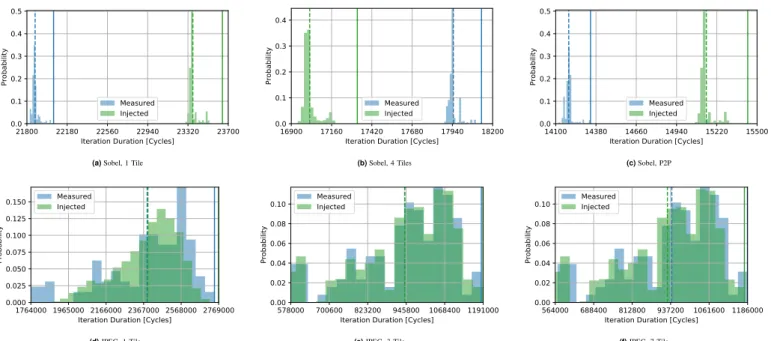
In Fig. 6, the measured (blue) and the simulated (green) distribution of the execution time of an iteration are presented. The dotted line marks the average execution time, the solid line the observed worst case. For the Sobel-Filter experiments the relative high error of up to 7.22 % (Sobel1, WCET) and −5.17 % (Sobel4, Average case) is visible. For the JPEG decoder the figure shows a better fitting of the simulated execu-tion times with the observed ones. Fig. 6 also demonstrates the advantages of considering the distribution of execution times. The distribution of the analyzed execution times come close to the distribution of the observed execution times.

In Tab. III the execution time to run the simulations is shown. We simulated with 1 000 000 computation time sam-ples for each actor. Each simulated experiment represents our 7 Tile platform with exception of the SobelP2P experiment.

The left column of Tab. III shows the simulation time considering the distribution of execution times. We simulated 1 000 000 iterations. For efficiency we split our simulation into 20 processes (each on a dedicated processor), each sim-ulating 50 000 iterations.

The middle column shows the worst case simulation con-sidering only the worst observed computation time for each actor. Since there is no variance in the computation time we simulated only 10 000 iterations. During these simulations we observed the worst case execution time (Tab. II, WC Simula-tion) at minimum of 715 times for the Sobel4 experiment.

21800 22180 22560 22940 23320 23700 Iteration Duration [Cycles]

0.0 0.1 0.2 0.3 0.4 0.5 Probability Measured Injected

(a) Sobel, 1 Tile

16900 17160 17420 17680 17940 18200 Iteration Duration [Cycles]

0.0 0.1 0.2 0.3 0.4 Probability Measured Injected (b) Sobel, 4 Tiles 14100 14380 14660 14940 15220 15500 Iteration Duration [Cycles]

0.0 0.1 0.2 0.3 0.4 0.5 Probability Measured Injected (c) Sobel, P2P 1764000 1965000 2166000 2367000 2568000 2769000 Iteration Duration [Cycles]

0.000 0.025 0.050 0.075 0.100 0.125 0.150 Probability Measured Injected (d) JPEG, 1 Tile 578000 700600 823200 945800 1068400 1191000 Iteration Duration [Cycles]

0.00 0.02 0.04 0.06 0.08 0.10 Probability Measured Injected

(e) JPEG, 3 Tile

564000 688400 812800 937200 1061600 1186000 Iteration Duration [Cycles]

0.00 0.02 0.04 0.06 0.08 0.10 Probability Measured Injected (f) JPEG, 7 Tile

Fig. 6. Distribution of the measured data (blue) compared to the results of the probabilistic simulation (green) for all experiments. The dashed lines show the median of the distribution, the solid lines the observed worst case.

103

104

105

106

Simulation runs [Iterations]

-2.0 -3.0 -4.0 -5.0 -1.0 0.0 1.0 2.0 3.0 4.0Error [%] -6.0 6.0 Injected Gaussian Uniform Distri. AVG WCET -5.68 -5.57 -5.75 -3.80 -0.80 -0.70 -0.70 1.69 0.15 1.70 1.70 1.70 0.77 0.45 6.07 17.71 0.16 0.22 0.17 0.16 0.79 17.71 23.48 -7.69

Fig. 7. Detailed analysis of the JPEG1 experiment. We compare Simulation runs to the error of the analysis results compared to the observed average and worst-case behavior for different distributions.

measure the actual execution time on the real platform. Again, 1 000 000 samples were measured.

The simulation time varies from a few seconds up to one hour for the JPEG7 experiment.

F. Discussion

In preliminary work [1], [13], [19] we compared different delay distribution of the simulated actors of our model regard-ing the error of the results. We repeated this experiment for the JPEG1 experiment because it is more compute intensive (Hypothesis H3) than the Sobel-Filter of our previous work. The results are presented in Fig. 7. Beside the distributions (Uniform (magenta), Gaussian (blue), Injected (teal)) we also varied the amount of simulation runs (Fig. 7 ordinate). We compared the results of the simulation with the observed behavior regarding average execution tile (filled data points) and WCET (outlined data points). The error is depicted on the abscissa of Fig. 7. The uniform distribution of delays between the observed BCET and WCET are suitable for quick WCET estimations but have a high error for the average case,

independent how many simulation runs are performed. The reason is that the average case of our applications is not in the center between their BCET and WCET. For our worst-case estimation (Tab. II, WC Simulation) we did 10 000 simulation runs using only one static delay. The Gaussian distribution is good for a quick average case estimation because the center point of the distribution is based on the mean value of our observed actor delays. The width of the Gaussian distribution leads to a very high over estimation of the WCET. The injected distribution, provides good average case and good worst case estimation. A downside is the need of many simulation runs to reduce the error. For our simulation using the injected distribution (Tab. II, Prob. Simulation) we did 1 000 000 simulation runs.

The static analytical model shows good results for appli-cation with high computational parts (Experiments JPEG1, JPEG3and JPEG7), because it benefits from our measurement based analysis of the execution times of each actor. The static analysis of the Sobel-Filter executed on 4 Tiles (Experiment Sobel4) has an error of 89.40 %. This is due to the fact, that the static model does not considers interleaving of execution phases of depending actors executed in parallel (Assumption A11). For the Sobel4 experiment, the actor GX could already start its read phase while GetPixel is still in its write phase, writing data on the channel to GY. For applications with short computation phases and long communication phases, this situation has a huge impact to the analyzed execution time.

Our simulation results are closer to the actual system because of the detailed communication model. Anyway, there is still a high error for the Sobel1 and Sobel4 experiments. The negative error of the Sobel4 and JPEG7 simulation may be due to an over optimistic communication model, because for the Sobel-Filter as well as for the highly parallel JPEG

decoder a good communication model is crucial.

The different worst case estimations of the WC

Simula-tion and Prob. Simulation are due to the different inputs

of the simulation. While the WC Simulation only uses one static delay for each actor (the worst observed delay), the probabilistic simulation uses the whole distribution of all observed execution times. In case of the JPEG1 experiment, this allows more than 1.17 × 1021 different combinations of actor delays which is not covered by our simulation. Therefore the combination of all worst actor delays may be not included in the 1 000 000 simulation runs. The Sobel4 experiment shows that considering only the worst case actor delays may not reveal the worst case iteration delay. Using the whole range of possible delays lead to a situation where the impact of the communication between actors caused a longer iteration time. The error of the SobelP2P experiment is because of lim-itations of our communication model. While our hypothesis

H2 is valid regarding the simplicity of the communication

hardware, the software to access the hardware FIFOs is hard to model because the processor architecture uses different instructions to access individual FIFOs. This leads to code with high branching behavior that is hard to represent in our communication model for the simulation [1] as well as the model used for our static analysis Sec III-D.

The results of our analysis also show, that the distance between the worst case and the average execution time of an iteration is low. For the Sobel-Filter, the reason is the small interval of the actual execution time (Sobel 1: 21802 . . . 22052, Sobel 4: 17887 . . . 18128). For the JPEG Decoder, in average the execution time is closer to the worst case than to the best case execution time as it can be seen in Fig. 6.

Fig. 6 also shows that our simulation comes close to the observed distributions, despite some offsets for the Sobel-Filter. The knowledge of the distribution of execution times can be used estimate how close the average case or the median is to the worst case. This can be useful for soft-real-time applications since it allows to estimate how often a certain deadline can be missed.

The JPEG experiments demonstrate the benefit of our approach for design space exploration. While increasing the number of tiles from 1 to 3 tiles with different accelerators, the execution time of an iteration decreased by the factor of 2.3 in average (Based on the Prob. simulation results in Tab. II). By further increasing the number of tiles to 7, so that each color channel of the JPEG image can be decoded in parallel, the average execution time only decreased by the factor of 1.01 compared to the 3 tile mapping. The JPEG decoder benefits from a heterogeneous 3 tile system compared to only 1 tile. Further tile have only little influence in the performance of the decoder and can be avoided to lower the hardware cost.

The fast simulation time (Tab. III) allows exploring differ-ent hardware configurations an mappings in short time. The comparison with the measurement time shows the benefit of our simulation. Beside the fact that the simulation makes the existing of the actual system needless, it is also faster than measuring each possible mapping. The reason for the long measurement time for the JPEG Decoder is the circumstance that the execution time of the decoder itself is very high For the

JPEG1 experiment, an iteration takes up to 2 746 197 cycles for the worst case. At a tile frequency of 100 MHz this is approximately 27 ms per iteration. For 1 000 000 samples the execution time can be up to 19 h. This is why the measurement time in Tab. III correlates with the execution times in Tab. II. Tab. III shows the simulation time for our experiments in hours. The low simulation times for the Sobel-Filter exper-iments and the JPEG-Decoder that got mapped on one Tile comes from the efficient communication between the actors. As long as no other actor is polling on data, the simulation can proceed the simulated time by the execution time of an actor. When there is an actor polling on data in parallel, then the simulation can only proceed by the time steps of the communication model. In our model, polling takes about 20 Cycles. If an actor polls on data of a preceding actor with an execution time of about 66 000 Cycles (GetMCU of the JPEG application) that gets executed in parallel, then the simulation gets slowed down by the factor of 3300. So the less polling is necessary for the simulated application, the faster the simulation is. An improvement of the simulated model (using events) and improving the communication model (more abstraction) can improve the simulation speed tremendously. This will remain future work.

V. CONCLUSION

In this paper we presented the benefits and limitations of our simulation based real-time analysis method. In com-parison with a static mathematical model, the error of our model is smaller. Furthermore does our method provide an approximation of the distribution of execution times for the analyzed system. The increasing simulation time for system with large application (long computation time) and many cores is currently limiting our approach to small systems.

Our approach is limited to tile-based multiprocessor sys-tems. To apply measurements to actors on this platform it furthermore must provide the necessary individual independent outputs. In our experiments we synthesized such a system on an FPGA. But there are also commercial off-the-shelf platforms available that fulfill these requirements [20].

The advantage of our approach is that our analysis not only estimates a WCET, but also provides an approximation of the distribution of possible execution times. Furthermore we use actual observed actor execution times as input which reduces the error of the analysis, because approximated func-tion can lead to execufunc-tion times that are outside the observed BCET/WCET boundaries (Gaussian distribution) or represent an unrealistic average execution time (Uniform distribution).

This allows us using a single tile (e.g. on a cheep evaluation board) for characterizing all actors of an application, and later decide, based on our simulations, how many tile in combination of different mappings and features are suitable for a specific application.

With our experiments we confirmed that our model is con-sistent and matches the reality with an error of less than 7.4 % for WCET estimation and 6.8 % for the average case. Our model needs some improvements to avoid negative errors for WCET analysis. For the average case, the negative errors are less critical. The accuracy in combination with the distribution

of possible execution times and fast analysis time our approach is very suitable for design space exploration.

VI. FUTUREWORK

In future work we plan to improve simulation quality as well as simulation speed by creating a more abstract commu-nication model and considering data dependencies to reduce the amount of simulation runs as well as lowering the error for some application. Our current communication model rep-resents communication in detail. A more abstract probabilistic model as used for the computation can increase simulation speed. We also did not consider any data dependency in our model. By considering data dependency, our model can not only be used for functional testing but also provides the possibilities to reduce simulation runs by avoiding redundancy and having a metric for determine the coverage of data paths. One further step would be reduce the required number of simulation runs with SMC methods. SMC methods, such as the Monte Carlo method, allow the number of simulation runs to be controlled with given level of confidence. By controlling the number of simulation runs, a trade-off between high con-fidence and fast analysis time is possible. The instrumentation and monitoring of SystemC models to carry out statistical analysis were presented in [21]. This approach could thus be adopted to quantitatively evaluate from the created models properties like the probability to miss a deadline.

In the context of WCET analysis, authors in [22], [23] proposed a measurement-based approach in combination with hardware and/or software randomization techniques to conduct a probabilistic worst-case execution time (pWCET) through the application of Extreme Value Theory (EVT). In future work we are going to analyze under which conditions (as-sumptions on the measurement and model calibration) we can apply EVT on our analytical execution time distributions to provide an analytic pWCET.

ACKNOWLEDGMENT

This work has been partially sponsored by the DAAD (PETA-MC project under grant agreement 57445418) with funds from the German Federal Ministry of Education and Re-search (BMBF). This work has also been partially sponsored by Campus France (PETA-MC project under grant agreement 42521PK) with funds from the French ministry of Europe and Foreign Affairs (MEAE) and by the French ministry for Higher Education, Research and Innovation (MESRI).

REFERENCES

[1] R. Stemmer, H.-D. Vu, K. Gr¨uttner, S. Le Nours, W. Nebel, and S. Pillement, “Experimental evaluation of probabilistic execution-time modeling and analysis methods for SDF applications on MPSoCs,” in 2019 International Conference on Embedded Computer Systems: Architectures, Modeling, and Simulation (SAMOS). Springer, 7 2019, pp. 241–254.

[2] S. Perathoner, E. Wandeler, L. Thiele, A. Hamann, S. Schliecker, R. Henia, R. Racu, R. Ernst, and M. Gonz´alez Harbour, “Influence of different abstractions on the performance analysis of distributed hard real-time systems,” Design Automation for Embedded Systems, vol. 13, no. 1, pp. 27–49, 2009.

[3] A. Gustavsson, A. Ermedahl, B. Lisper, and P. Pettersson, “Towards WCET analysis of multicore architectures using UPPAAL,” in WCET, 2010, pp. 101–112.

[4] G. Giannopoulou, K. Lampka, N. Stoimenov, and L. Thiele, “Timed model checking with abstractions: Towards worst-case response time analysis in resource-sharing manycore systems,” in Proc. International Conference on Embedded Software (EMSOFT). Tampere, Finland: ACM, 10 2012, pp. 63–72.

[5] M. Fakih, K. Gr¨uttner, M. Fr¨anzle, and A. Rettberg, “State-based real-time analysis of SDF applications on mpsocs with shared communication resources,” Journal of Systems Architecture - Embedded Systems Design, vol. 61, no. 9, pp. 486–509, 2015.

[6] A. Legay, B. Delahaye, and S. Bensalem, “Statistical model check-ing: An overview,” in Runtime Verification, H. Barringer, Y. Falcone, B. Finkbeiner, K. Havelund, I. Lee, G. Pace, G. Ros¸u, O. Sokolsky, and N. Tillmann, Eds. Berlin, Heidelberg: Springer Berlin Heidelberg, 2010, pp. 122–135.

[7] A. David, K. G. Larsen, A. Legay, M. Mikucionis, D. B. Poulsen, J. van Vliet, and Z. Wang, “Statistical model checking for networks of priced timed automata,” in Formal Modeling and Analysis of Timed Systems, ser. Lecture Notes in Computer Science, U. Fahrenberg and S. Tripakis, Eds. Springer Berlin Heidelberg, 2011, vol. 6919, pp. 80–96. [8] M. Kwiatkowska, G. Norman, and D. Parker, “Prism 4.0: Verification

of probabilistic real-time systems,” in In Proc. International Conference on Computer Aided Verification (CAV’11), 7 2011, pp. 585–591. [9] C. Jegourel, A. Legay, and S. Sedwards, “A platform for high

perfor-mance statistical model checking - plasma,” in In Proc. International Conference Tools and Algorithms for the Construction and Analysis of Systems (TACAS’12), 2012, pp. pp.498 – 503.

[10] A. Nouri, M. Bozga, A. Moinos, A. Legay, and S. Bensalem, “Building faithful high-level models and performance evaluation of manycore embedded systems,” in ACM/IEEE International conference on Formal methods and models for codesign, 2014.

[11] A. Nouri, S. Bensalem, M. Bozga, B. Delahaye, C. Jegourel, and A. Legay, “Statistical model checking qos properties of systems with sbip,” International Journal on Software Tools for Technology Transfer, p. pp. 14, 2014.

[12] M. Chen, D. Yue, X. Qin, X. Fu, and P. Mishra, “Variation-aware evaluation of mpsoc task allocation and scheduling strategies using statistical model checking,” in 2015 Design, Automation Test in Europe Conference Exhibition (DATE), March 2015, pp. 199–204.

[13] R. Stemmer, H. Schlender, M. Fakih, K. Gr¨uttner, and W. Nebel, “Probabilistic state-based RT-analysis of SDFGs on MPSoCs with shared memory communication,” in 2019 Design, Automation & Test in Europe Conference & Exhibition (DATE), 3 2019.

[14] C. Schlaak, M. Fakih, and R. Stemmer, “Power and execution time measurement methodology for sdf applications on fpga-based mpsocs,” arXiv preprint arXiv:1701.03709, 2017.

[15] E. A. Lee and D. G. Messerschmitt, “Synchronous data flow,” Proceed-ings of the IEEE, vol. 75, no. 9, pp. 1235–1245, 1987.

[16] A. Shabbir, A. Kumar, S. Stuijk, B. Mesman, and H. Corporaal, “Ca-mpsoc: An automated design flow for predictable multi-processor architectures for multiple applications,” Journal of Systems Architecture, vol. 56, no. 7, pp. 265–277, 2010.

[17] R. Hoes, “Predictable dynamic behaviour in noc-based multiprocessor system-on-chip,” Master’s Thesis, Eindhoven University of Technology, Eindhoven (The Netherlands), 2005.

[18] M. Galassi, J. Davies, J. Theiler, B. Gough, G. Jungman, P. Alken, M. Booth, F. Rossi, and R. Ulerich, “The gnu scientific library reference manual, 2007,” URL http://www.gnu.org/software/gsl, 2007.

[19] R. Stemmer, H.-D. Vu, M. Fakih, K. Gr¨uttner, S. Le Nours, and S. Pillement, “Feasibility Study of Probabilistic Timing Analysis Methods for SDF Applications on Multi-Core Processors,” IETR ; OFFIS, Research Report, Mar. 2019. [Online]. Available: https: //hal.archives-ouvertes.fr/hal-02071362

[20] P. Inc. (2019) Parallax propeller. [Online]. Available: https://www. parallax.com/microcontrollers/propeller

[21] V. C. Ngo, A. Legay, and J. Quilbeuf, “Statistical model checking for systemc models,” in IEEE 17th International Symposium on High Assurance Systems Engineering (HASE), 2016, pp. pp.197–204. [22] F. J. Cazorla, E. Qui˜nones, T. Vardanega, L. Cucu, B. Triquet, G. Bernat,

E. Berger, J. Abella, F. Wartel, M. Houston et al., “Proartis: Probabilis-tically analyzable real-time systems,” ACM Transactions on Embedded Computing Systems (TECS), vol. 12, no. 2s, p. 94, 2013.

[23] F. J. Cazorla, J. Abella, J. Andersson, T. Vardanega, F. Vatrinet, I. Bate, I. Broster, M. Azkarate-Askasua, F. Wartel, L. Cucu et al., “Proxima: Improving measurement-based timing analysis through randomisation and probabilistic analysis,” in Digital System Design (DSD), 2016 Euromicro Conference on. IEEE, 2016, pp. 276–285.