Quantification of Neural Network Uncertainties on the Hydrogeological Predictions by Probability Density Functions

(1)

HAL Id: hal-02366200

https://hal.archives-ouvertes.fr/hal-02366200

Submitted on 15 Nov 2019

HAL is a multi-disciplinary open access archive for the deposit and dissemination of sci-entific research documents, whether they are pub-lished or not. The documents may come from teaching and research institutions in France or abroad, or from public or private research centers.

L’archive ouverte pluridisciplinaire HAL, est destinée au dépôt et à la diffusion de documents scientifiques de niveau recherche, publiés ou non, émanant des établissements d’enseignement et de recherche français ou étrangers, des laboratoires publics ou privés.

Distributed under a Creative Commons Attribution| 4.0 International License

Quantification of Neural Network Uncertainties on the

Hydrogeological Predictions by Probability Density

Functions

Nicolas Akil, Guillaume Artigue, Michael Savary, Anne Johannet, Marc

Vinches

To cite this version:

Nicolas Akil, Guillaume Artigue, Michael Savary, Anne Johannet, Marc Vinches. Quantification of Neural Network Uncertainties on the Hydrogeological Predictions by Probability Density Functions. WMESS 2019 - 5th World Multidisciplinary Earth Sciences Symposium, Sep 2019, Prague, Czech Republic. �10.1088/1755-1315/362/1/012112�. �hal-02366200�

(2)

IOP Conference Series: Earth and Environmental Science

PAPER • OPEN ACCESS

Quantification of Neural Network Uncertainties on the Hydrogeological

Predictions by Probability Density Functions

To cite this article: Nicolas Akil et al 2019 IOP Conf. Ser.: Earth Environ. Sci. 362 012112

(3)

Content from this work may be used under the terms of theCreative Commons Attribution 3.0 licence. Any further distribution of this work must maintain attribution to the author(s) and the title of the work, journal citation and DOI.

Published under licence by IOP Publishing Ltd

World Multidisciplinary Earth Sciences Symposium (WMESS 2019) IOP Conf. Series: Earth and Environmental Science 362 (2019) 012112

IOP Publishing doi:10.1088/1755-1315/362/1/012112

1

Quantification of Neural Network Uncertainties on the

Hydrogeological Predictions by Probability Density Functions

Nicolas Akil1,2_{, Guillaume Artigue}1_{, Michael Savary}2_{, Anne Johannet}1_{, Marc} Vinches1

1_{LGEI, IMT Mines Alès, Univ. Montpellier, 6 Avenue de Clavières. 30319 Alès} Cedex FRANCE

2_{AQUASYS, 2 rue de Nantes, 44710 Port-Saint-Père FRANCE}

guillaume.artigue@mines-ales.fr

Abstract. The risk of drought impacting the drinking water and agricultural production is worrying in the developed countries, especially in a changing climate context. To manage and prevent this phenomenon, real-time monitoring and predictive systems are emerging as the key solutions. In the field of artificial intelligence, neural networks are one of these predictive systems. This family of parameterized models is a composition of neuronal functions, which apply a non-linear transformation from their inputs to their outputs. These networks are able to learn a hydro(geo)logical system behaviour using a database composed of observed inputs (rainfall, evapotranspiration, etc.) and outputs (groundwater level, discharge, etc.), thanks to an algorithm minimizing a cost function between observed and simulated outputs. However, it remains difficult to assess the uncertainty generated by these models, possibly leading to misinterpretations by the end users. These uncertainties are mainly of three types. The first is related to the input data. Indeed, hydrosystems are surface elements whereas meteorological inputs are punctual elements. The interpolation error can, therefore, be significant because of the lack of knowledge between gauging stations. The second is the neural network model architecture itself. It is possible to deal with this source of uncertainty using regularization methods. Finally, the neural networks are submitted to uncertainties related to parameter initialization, before the training step. The initial parameters may have an important impact on the results. In this paper, we address the prediction of the Blavet groundwater level (Bretagne, France). In order to assess uncertainties, we will first focus on the parameters initialization of the model. Neuronal models are optimized using cross-validation and early stopping. Then, an ensemble model is realized, in which each member is the result of a unique set of parameters initialization. The purpose of the study is to define how many initializations are necessary to obtain a reasonable confidence interval for forecasts, with the smallest interval and the higher rate of observed points inside this interval. The best model will be determined using cross-validation scores thereby ensuring optimal robustness. We show that, in this case study, an ensemble model of 20 different initializations is sufficient to estimate uncertainty while preserving quality. In the second part, the resulting ensemble model will be used to estimate the global model uncertainty using probability density functions (pdf) applied to the distribution of groundwater level data and cross-validation scores of forecasts. It reveals that the groundwater level predictions are composed of two mixed distributions. Therefore, we will use the expectation-maximization algorithm (EM) to obtain parameters of mixed models. Mixed normal and mixed Gumbel laws, among five mixed distributions assessed, give the best groundwater distribution and are able to generate an abacus drawing uncertainty of model.

(4)

1. Introduction

Water related risks impact a large part of the population. On the one hand, floods frequently cause fatalities and damages. On the other hand, droughts affect drinking water and agricultural production. In a climate change context, with a rise of extreme phenomena frequency and duration [1], real-time monitoring and predictive systems are emerging as key solutions. To forecast the underground water level or river discharge, two main solutions emerge. The first relies on a deep knowledge of the considered system, dedicated to building physically based models. Unfortunately, this knowledge is most of the time difficult to acquire, leading to lower efficiency and high time and money consuming methods. The second one relies on the relation between system inputs and outputs, never making any strong hypothesis on the system operation, as long as the inputs are able to explain the outputs (such as rainfall for discharge). In the latter solution family, neural networks play an important role as they are known to be able to identify dynamical processes [2]. However, like any model would do, they generate uncertainties which are sometimes difficult both to quantify and to express, and can lead to misinterpretations by end users. These uncertainties mainly have three origins: input data (especially noise and spatial variability), model architecture and parameters initialization before the training step [3].

In the present paper, we propose a methodology to allow quantifying some of these uncertainties. The first part consists of building a reliable model to forecast groundwater level on a case study of north-western France. As [4] did with success on a southern France karst aquifer, the neural model will be optimized using cross-validation and early stopping. In the targeted region, we will state that the high quality of data and the low spatial variability are good enough reasons to overlook the uncertainties coming from data. Besides, the strict application of regularization methods should protect us from the uncertainties coming from the model architecture. We will thus focus on parameters initialization uncertainties, which are consequently considered as the main source of uncertainty in this case. The second part will consist of assessing this uncertainty, by generating ensemble models composed of members corresponding to different random sets of initial parameters. At last, the uncertainty will be expressed as a function of the state of the system in order to build an uncertainty pattern using statistical distributions. After having reminded the main characteristics of neural models and having presented the study area, we will describe more precisely the methodology used and discuss the results obtained.

2. Neural networks

2.1 Background

A neuron is a mathematical operator applying a nonlinear transformation from its inputs to its outputs. In practice, it makes a weighted sum of its inputs transformed by an activation function thus giving an output. The weights of the sum are the parameters of the neural network.

Neurons can be combined in networks following architecture depending on: (i) the data describing the modelled system, and (ii) the purpose of the model. Neurons are then organised in layers of two types: output layers, whose outputs are the outputs of the model, and associated to measured values, and hidden layers, whose outputs are not associated to measured values [5].

2.2 Neural networks models

Depending on how they deal with time, neural networks can be called “static” or “recurrent”. In the first case, time does not play any functional role and the input variables are exogenous (static model, (1)).

𝑦𝑦�(𝑘𝑘) = 𝜑𝜑(𝐱𝐱(𝑘𝑘), … , 𝐱𝐱(𝑘𝑘 − 𝑛𝑛𝑟𝑟+ 1), 𝐖𝐖) (1)

Where 𝑦𝑦�(𝑘𝑘) is the estimated output at the discrete time k; 𝜑𝜑 the nonlinear function implemented by the model; 𝒙𝒙 the input vector; 𝑛𝑛𝑟𝑟 the sliding time windows size that defines the length of the necessary

(5)

3

In the second case, added to the exogenous variables, the result of the simulation at the previous time steps is used as an input variable (recurrent model, (2)).

𝑦𝑦�(𝑘𝑘) = 𝜑𝜑(𝒚𝒚�(𝑘𝑘 − 1), … , 𝒚𝒚�(𝑘𝑘 − 𝑟𝑟); 𝒙𝒙(𝑘𝑘), … , 𝒙𝒙(𝑘𝑘 − 𝑛𝑛𝑟𝑟+ 1), 𝐖𝐖) (2)

Where 𝑟𝑟 is the order of the recurrent model.

A third case, called “feed-forward model” substitutes the recurrent input by the observations of the output at the previous time steps (3).

𝑦𝑦�(𝑘𝑘) = 𝜑𝜑(𝒚𝒚(𝑘𝑘 − 1), … , 𝒚𝒚(𝑘𝑘 − 𝑟𝑟); 𝒙𝒙(𝑘𝑘), … , 𝒙𝒙(𝑘𝑘 − 𝑛𝑛𝑟𝑟+ 1), 𝐖𝐖) (3)

Where 𝒚𝒚(𝑘𝑘) is the observed value of the simulated variable at the discrete time k.

Recurrent models are used when the noise affecting outputs is known to be higher than the one affecting inputs. In contrast, feed-forward models, in which previously observed outputs are used as input variables, are used when the noise affecting input data is known to be the highest [6, 7].

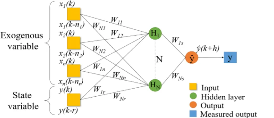
One of the most common neural network structures is a feed-forward model called “multilayer perceptron” (MLP), for which the universal approximation property has been shown by [8]. This property mainly states that that kind of model (Figure 1) can approach any differentiable function as soon as it has enough hidden neurons and a database of sufficient quality.

Figure 1. Multilayer Perceptron representation, with xi, the

exogenous variables, Wab, the

parameters, y, the measured output, ŷ, the simulated output, r, the order of the model, nr, the

input window width, HN, hidden

neuron, N, the number of hidden neurons, k, the discrete time and h, the lead time

Beside this property, a MLP also has the parsimony property, shown by [9], that states that if the function operated by the model depends on nonlinearly adjustable parameters, it is more parsimonious than if it depends linearly on its parameters. This property is even more valuable when the number of input variables increases.

2.3 Neural networks training and overtraining: regularization methods

Training a neural network means finding the parameters vector such as a cost function is minimized. A training data set is dedicated to this task and a training algorithm is implemented. The purpose is to find the best approximation of the regression function to make the model adjust itself to the training set. Consequently, a too complex model will adapt to the signal and to the random noise carried by this signal. On the other hand, a too simple model will not be able to adapt to the signal. This is called the “bias/variance dilemma” [10]. If the bias decreases too much, there is a risk that the model is adjusting to the noise, thus increasing the variance of its output, whereas a low variance and a low bias are desired. Therefore, the error on the training set is not a relevant estimator of the generalisation error.

We understand here that the result is highly depending on the data contained in the training set. To assess the generalization error of the model, one can use cross-validation [11]. Applied to the increasing

(6)

model complexities, it provides a performance score that should decrease while the score the model obtains on the training set still increases, showing that the model performances in generalization are becoming too complex. Also, to stop training before the generalization capability decreases, one can use early stopping [12], which consists of applying the model to a separate smaller data set and to stop training when the cost function reaches a minimum on this set.

In this paper, both these regularization methods will be applied, in order to ensure the robustness of the model [13]. Beside these issues, the neural models are sensitive to the initial random values of the parameters at the beginning of the training step. The modeller thus has to ensure that the result given by a model is robust and not depending on this random initialization. A certain number of these initializations may be used to create an ensemble that provides a range of possibilities [5, 14].

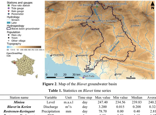
3. Study area: the Blavet groundwater basin

Located in north-western France, in the Bretagne region, the Blavet groundwater basin lies on more than 2,100 sq.km. It is mainly composed of metamorphic, magmatic and sandy rocks and its elevation ranges from -15 to 320 m.a.s.l. (Figure 2). Due to the low porosity of bedrock, this groundwater only exists thanks to regoliths and faults [15].

Figure 2. Map of the Blavet groundwater basin Table 1. Statistics on Blavet time series

Station name Variable Unit Time step Max value Min value Median Average

Miniou Level m.a.s.l day 247.40 234.56 239.83 240.21

Blavet in Kerien Discharge m3_/s _day _3.200 _0.015 _0.208 _0.325

Rostrenen-Keringant Precipitation mm day 78.70 0.00 0.40 2.81

Rostrenen-Keringant PET mm day 8.90 0.00 1.60 1.87

Data range from 2005 to 2019 at a daily time-step. They are issued from a meteorological station in Rostrenen (temperature, precipitation and evapotranspiration), a piezometer and a discharge station are also located in Rostrenen (Table 1). It has been shown that groundwater contributed at 57 % to river discharge at Blavet in Kerien during the 1994 to 2000 period [16]. Therefore, strong interactions between groundwater and surface water exist in this basin. From a climate point of view, the area is submitted to an oceanic climate, with an annual mean rainfall from 900 to 1,300mm and moderate temperatures, based on the 1981 to 2010 averages (Météo France).

(7)

5

4. Methodology

4.1 Variable selection

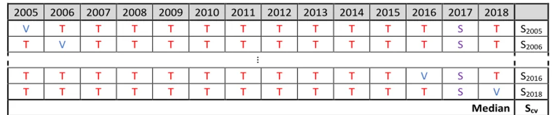
Inputs are divided in a one-year-long-subsets, from January to December, except for first and last years that are not complete. These subsets are used for training, except for the one used for stop set (2017) and the one used for validation set that ranges from the end of 2018 to the beginning of 2019 (5 months). As the groundwater levels are available, a feed-forward model seems convenient. We also state that the water level measurement is accurate while rainfall and evapotranspiration measurements are not as much accurate, especially considering that there is only one meteorological station for a large surface and only one discharge station. In order to design the range of sliding input time windows (see section 2.2) that will be used for the model selection, cross correlations between available inputs and the output are calculated. They provide information on the explanatory power of the inputs on the outputs. They also show the response time, the memory effect of the system and the reasonable lead-time that could be reached. This lead-time is 3 days, which is long enough to make the output varying, and short enough to preserve forecast quality, even in the absence of rainfall forecast.

4.2 Complexity selection

To ensure the robustness of the model, we explore different architectures and apply cross-validation. We thus select the depth of the sliding input time windows along with the complexity of the model. The cross-validation score SCV is obtained by the median of the scores calculated for each combination of training / validation sets (Figure 3).

Figure 3. Schematic view of the cross-validation process; T is for training, V for validation, S for stop; Syyyy is for the score calculated on the yyyy subset, SCV is for the median of the scores The score can be any relevant indicator of the performance. In the case of forecasting low variability variables, the persistence criterion [17] that measures the difference between a naïve forecast and the calculated forecast, is well suited (4).

𝐶𝐶𝑃𝑃= 1 − ∑ (𝑌𝑌𝑝𝑝,𝑘𝑘+ℎ−𝑌𝑌𝑠𝑠,𝑘𝑘+ℎ)² 𝑛𝑛

𝑘𝑘

∑ (𝑌𝑌𝑛𝑛𝑘𝑘 𝑝𝑝,𝑘𝑘−𝑌𝑌𝑝𝑝, 𝑘𝑘+ℎ)² (4)

Where 𝑌𝑌𝑝𝑝,𝑘𝑘 is the measured value at the discrete time k, 𝑌𝑌𝑠𝑠,𝑘𝑘 is the predicted value at the discrete time k and 𝑌𝑌𝑝𝑝, 𝑘𝑘+ℎ the observed value at the discrete time k+h, with h, the lead time.

This selection process is applied for all the possible relevant architectures in conjunction with early stopping. Variables and complexity are thus appropriately selected, using a relevant score for the purpose of this study.

4.3 Parameters initialization

After training, the parameters of the model possibly depend on their initial random value. Un uncertainty on the results is generated. The purpose of this study is to quantify this uncertainty, providing a range of possible outputs, called the prediction interval. This interval must be as small as possible (measured by the MPI criterion (Mean Prediction Interval), [18]) whereas it includes a maximum of observed values (which is measured by the PICP criterion (Prediction Interval Coverage Probability) [18]). The purpose of this step is to define how many random initializations are necessary to reach this optimum that will be calculated using SFPI (Spatial Frequency Prediction Interval) (5).

2005 2006 2007 2008 2009 2010 2011 2012 2013 2014 2015 2016 2017 2018 V T T T T T T T T T T T S T S2005 T V T T T T T T T T T T S T S2006 … T T T T T T T T T T T V S T S2016 T T T T T T T T T T T T S V S2018 Median Scv

(8)

IOP Publishing doi:10.1088/1755-1315/362/1/012112 𝐶𝐶𝑆𝑆𝑆𝑆𝑃𝑃𝑆𝑆=𝐶𝐶_𝐶𝐶𝑃𝑃𝑆𝑆𝑃𝑃𝑃𝑃 𝑀𝑀𝑃𝑃𝑆𝑆 = 1 𝑛𝑛 ∑ 𝑓𝑓(𝑌𝑌𝑛𝑛𝑘𝑘 𝑝𝑝,𝑘𝑘) 1 𝑛𝑛 ∑ (𝑌𝑌𝑛𝑛𝑘𝑘 𝑠𝑠𝑚𝑚𝑚𝑚𝑚𝑚,𝑘𝑘− 𝑌𝑌𝑠𝑠𝑚𝑚𝑚𝑚𝑛𝑛,𝑘𝑘) with 𝑓𝑓(𝑌𝑌𝑝𝑝,𝑘𝑘) = 1 if 𝑌𝑌𝑝𝑝,𝑘𝑘 ∈ [𝑌𝑌𝑠𝑠𝑚𝑚𝑚𝑚𝑛𝑛,𝑘𝑘; 𝑌𝑌𝑠𝑠𝑚𝑚𝑚𝑚𝑚𝑚,𝑘𝑘], else 𝑓𝑓(𝑌𝑌𝑝𝑝,𝑘𝑘) = 0 (5) Where 𝑌𝑌𝑝𝑝,𝑘𝑘 is the measured value at the discrete time k and 𝑌𝑌𝑠𝑠𝑚𝑚𝑚𝑚𝑛𝑛,𝑘𝑘 and 𝑌𝑌𝑠𝑠𝑚𝑚𝑚𝑚𝑚𝑚,𝑘𝑘 the upper and lower bounds of the forecast interval.

Ensemble forecasts are thus calculated, with 3 to 120 members in each (respectively 3, 5, 10, 20, 30, 40, 50, 60, 80, 100 and 120 forecasts). For each of these intervals, the SFPI criterion is calculated, allowing defining an optimal number of initializations with a relevant benchmark.

4.4 Representation of model uncertainty with probability density functions (pdf)

The uncertainty can be approached with pdf applied to output variable distribution. For this purpose, we fit 5 different pdf to the observed groundwater level distributions, which are Normal [19], Gumbel [20], Laplace [21], Cauchy [22] and Logistic laws [23], detailed respectively in (6), (7), (8), (9) and (10).

𝒩𝒩(𝑥𝑥̅, 𝜎𝜎2_{) =} 1 𝜎𝜎√2𝜋𝜋 𝑒𝑒− (𝑚𝑚−𝑚𝑚�)² 2𝜎𝜎² (6) 𝒢𝒢𝒢𝒢𝒢𝒢(𝑥𝑥̅, 𝛽𝛽) =𝑒𝑒−(𝑚𝑚−𝑚𝑚�)𝛽𝛽 𝑒𝑒−𝑒𝑒 −(𝑚𝑚−𝑚𝑚�)_𝛽𝛽 𝛽𝛽 (7) ℒ𝒶𝒶𝒶𝒶(𝑥𝑥̅, 𝑏𝑏) =_2𝑏𝑏1 𝑒𝑒−(|𝑚𝑚−𝑚𝑚�|)𝑏𝑏 (8) 𝒞𝒞𝒶𝒶𝒢𝒢(𝑥𝑥0, 𝑎𝑎) = 1 𝜋𝜋𝜋𝜋 (1+�𝑚𝑚 − 𝑚𝑚0 _𝑚𝑚 �2) (9) ℒ𝑜𝑜𝑜𝑜𝒾𝒾𝒾𝒾𝒾𝒾(𝑥𝑥̅, 𝑠𝑠) = 𝑒𝑒−(𝑚𝑚−𝑚𝑚�)𝑠𝑠 𝑠𝑠 �1+𝑒𝑒−(𝑚𝑚−𝑚𝑚�)𝑠𝑠 _� 2 (10)

Where x is the variable,x its mean, x0, its median, σ² its variance and a, b, β and s scale parameters.

In the case of Blavet groundwater level, a double distribution appears, corresponding to dry and wet seasons, leading to finding a mixed distribution. An expectation-maximization algorithm is applied to the 5 laws described, to obtain pdf parameters. The main purpose of this algorithm is to find a maximum likelihood set of parameters of a model when equations are not solvable. This algorithm is established in two steps. The first is the expectation step, where an expected value for log-likelihood parameters is defined, following assessed distribution or pdf. The second step is the maximization step, which consists of obtaining parameters that maximize the expected value, using an iterative process [24]. After finding parameters of each pdf, their inflection point is obtained, which allows separating mixed distribution in two pdf. Each pdf is multiplied by PICP, thus giving pdf of distribution included in prediction interval, by addition of the two pdf. The same process is used for water levels outside the prediction interval. It is lastly possible to rebuild mixed pdf, by addition of outside pdf and included pdf. The ratio between included prediction interval pdf and summoned pdf is calculated in order to obtain the probability to have a forecast inside the prediction interval for each groundwater level.

5. Results and discussions

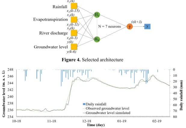
5.1 Model selected and deterministic results

The model selected by the combined variable and complexity selection processes, especially cross-validation with the persistence criterion has the architecture presented in Figure 4. This model is

(9)

7

validated on the test set, which is totally unknown of the model, and gives the results shown in Figure 5, with Cp = 0.65. These results are qualitative enough to assess uncertainties without being dependent on the errors of the model.

Figure 4. Selected architecture

Figure 5. Validation of groundwater level forecasting at 3 days lead-time on the test set 5.2 Optimal number of initializations and ensemble results

Once the architecture is selected and the model validated, ensemble forecasts are calculated. The number of members varies as described in section 4.3 while the performance is assessed using the SFPI criterion as a cross validation score.

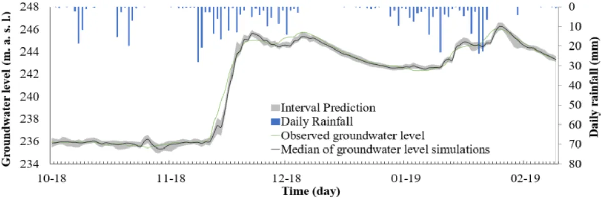
Figure 6. SFPI cross-validation score of ensemble models as a function of the number of members As observed in Figure 6, a close to optimum performance is reached for 20 initializations. Even if the SFPI could be enhanced by using more members, the cost-benefit ratio (especially regarding calculation time) pleads in favour of the 20 members. Figure 7 shows the result for the test event, with a median PICP of 90% and an MPI of 0.41m, it reaches an SFPI of 1.25.

(10)

Figure 7. Representation of Figure 5 forecast with a prediction interval 5.3 Representation of uncertainties

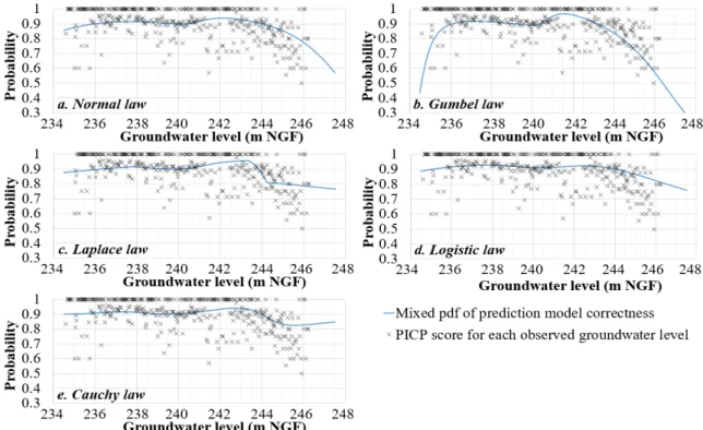
First, we need to focus on the ensemble forecast groundwater distribution. It shows higher occurrence frequencies for wet and dry periods (resp. >242 m.a.s.l. and <238 m.a.s.l.). Intermediate values are less frequent because of the quick evolution of levels occurring in them. Consequently, it appears that groundwater distribution is a double distribution and that an expectation-maximisation algorithm is needed to separate both pdf. We obtain inflexion points for each of the calculated laws that can be seen in Figure 8 and that range from 240.52 to 240.76 m.a.s.l. Using these values, mixed pdf are calculated and compared to groundwater distributions inside and outside the interval.

Figure 8. Mixed pdf of groundwater distributions. Determination coefficients are indicated in graphs (“In” means inside prediction interval, “out” means outside and “Cor.” is model correctness) The final step consists of calculating the abacus of model correctness, which is presented in Figure 9, comparing the calculated pdf with PICP scores observed for each piezometer level. PICP scores are ignored if they appear less than 3 times in the whole set. Except for Cauchy mixed pdf, each pdf is decreasing when approaching the extreme values. Normal, Gumbel and logistic mixed pdf seems to be the best of the 5 mixed laws, especially considering their determination coefficients. They also fit with observed groundwater level distributions. It remains a high uncertainty on the calculation of model correctness probability, determination coefficients rarely exceeding 0.5. Furthermore, PICP scores cannot be calculated for the highest groundwater levels, due to their low representation in the data set. This implies that abacus cannot ensure a reliable probability prediction for these levels. Lastly, this methodology requires large datasets, in order to have enough examples of high droughts or floods.

(11)

9

Figure 9. Abacus of mixed pdf of model correctness

6. Conclusions

This methodology allows forecasting neural network model uncertainty in the case of low uncertainty coming from the data and from the model architecture. This low uncertainty comes from a rigorous variable and complexity selection, applied to ensure the robustness of the model. The initialization of the parameters during the training step of the model is thus considered as the main source of uncertainty and it is first represented by ensemble forecasts, whose number of members must be defined as a function of the purpose of the model.

The use of the abacus created thanks to the law distribution fitting provides a significantly good representation of model uncertainty. With this abacus, it is possible to extrapolate uncertainties to unobserved value. The abacus is based on frequency distribution and as expected, it leads to: (i) a data set size sensibility and (ii) a low accuracy for an extreme event. Despite this limitation, this method is shown in our study, the possibility to use two different distribution laws; normal law and logistic law. Thanks to this final observation, the future work will focus on the application of multi-law distribution representation for the prediction uncertainty.

Acknowledgments

Authors would like to warmly thank the BRGM, which provided the dataset, J. Nicolas (BRGM) and S. Pistre (Univ. Montp.) for helpful discussions and the ANRT, which contributed to funding this work. References

[1] D. L. Hartmann, “Observations: Atmosphere and Surface”, Climate Change 2013: The Phys. Sc. Basis. Cont. of WG I to the 5th Ass. Report of the Inter. Panel on CC, 2, pp 159–254, 2013. [2] L. Kong-A-Siou, “Neural networks for karst groundwater management: case of the Lez spring

(Southern France)”, Env. Earth Sciences, Volume: 74 Issue: 12, 7617-7632, 2015.

[3] F. Bourgin, “Comment quantifier l’incertitude prédictive en modélisation hydrologique? Travail exploratoire sur un grand échantillon de bassins versants”, PhD Thesis, AgroParisTech, 230 p., HAL: tel-01130084, v. 2, 2014.

(12)

[4] L. Kong-A-Siou, A. Johannet, V. Estupina-Borrell, and S. Pistre, “Optimization of the generalization capability for rainfall–runoff modeling by neural networks: the case of the Lez aquifer (southern France)”, Environmental Earth Sciences, 65(8), 2365-2375, 2012.

[5] G. Dreyfus, Neural networks, Methodology and applications, Springer, Berlin, 2005.

[6] O. Nerrand, P. Roussel-Ragot, L. Personnaz, G. Dreyfus, and S. Marcos, “Neural Networks and Nonlinear Adaptive Filtering: Unifying Concepts and New Algorithms.", Neural Comp 5(2), 165-199, 1993.

[7] V. Taver, A. Johannet, V. Borrel-Estupina, and S. Pistre, “Feed-forward vs recurrent neural network models for non-stationarity modelling using data assimilation and adaptivity”, HSJ – J. des Sciences Hydrologiques, Vol. 60, Issue 7-8, Special Issue, 1242-1265, 2015.

[8] K. Hornik, M. Stinchombe and H. White, “Multilayer Feedforward Networks are Universal Approximators”, Neural Networks, vol. 2, pp. 359–366, 1989.

[9] A. R. Barron, "Universal Approximation Bounds for Superpositions of a Sigmoidal Function." IEEE Trans. Inf. Theor. 39 (3): 930-45, 1993.

[10] S. Geman, E. Bienenstock and R. Doursat, “Neural Networks and the Bias/Variance dilemma”, Neural Computation, vol. 4, pp. 1–58, 1992.

[11] M. Stone, “Cross-Validatory Choice and Assessment of Statistical Predictions”, Journal of the Royal Statistical Society, Series B (Methodological), vol. 36, no. 2, pp. 111–147, 1974. [12] J. Sjöberg, Q. Zhang, L. Ljung, A. Benveniste, B. Delyon, P. Y. Glorennec, H. Hjalmarsson and

A. Juditsky, “Nonlinear Black-box Modeling in System Identification: a unified overview”, Automatica, vol. 31, no. 12, pp. 1691–1724, 1995.

[13] L. Kong-A-Siou, A. Johannet, V. Estupina-Borrell, and S. Pistre, “Optimization of the generalization capability for rainfall–runoff modeling by neural networks: the case of the Lez aquifer (southern France)”, Environmental Earth Sciences, 65(8), 2365-2375, 2012.

[14] T. Darras, A. Johannet, B. Vayssade, L. Kong-A-Siou and S. Pistre, “Influence of the Initialization of Multilayer Perceptron for Flash Flood Forecasting: Design of a Robust Model.”, International Work-Conference on Time Series Analysis, 12 pp., 225–235, 2014.

[15] F. Lucassou and B. Mougin, “Essai d’élaboration d’indicateurs piézométriques pour la gestion quantitative AEP dans le département des Côtes d’Armor – Rapport final”, BRGM, RP-53326-FR, 80 pp., 2015.

[16] B. Mougin, A. Carn, N. Debeglia, J. Perrin and E. Thomas, “SILURES Bretagne (Système d’Information pour la Localisation et l’Utilisation des Ressources en Eaux Souterraines)”, BRGM, RP-52825-FR, 62 pp., 2004.

[17] P. K. Kitanadis and R. L. Bras, “Real-time forecasting with a conceptual hydrologic model: 2. Applications and results.”, Water Resources Research, vol. 16, no. 6, pp. 1034–1044, 1980. [18] D. L. Shrestha and D. P. Solomatine, “Machine learning approaches for estimation of prediction

interval for the model output.”, Neural Networks, vol. 19, pp. 225–235, 2006.

[19] R. A. Fisher, “On the mathematical foundations of theoretical statistics”, Philosophical Transactions of the Royal Society, vol. 9, no. 222, pp. 309–368, 1922.

[20] E. J. Gumbel, “Méthodes graphiques pour l’analyse des débits de crues”, Revue de statistique appliquée, vol. 5, no. 2, pp. 77–89, 1957.

[21] P. S. Laplace, “Mémoire sur la probabilité des causes par les évènements”. Mémoires de l’Academie Royale des Sciences, Presentés par Divers Savan, vol. 6, pp. 621–656, 1774. [22] A. L. Cauchy, “Sur les résultats moyens d’observations de même nature, et sur les résultats les

plus probables”. Comptes Rendus Hebd. Seances Acad. Sci. Paris, vol. 37, pp. 198–206, 1853. [23] P. F. Verhulst, “Recherches mathématiques sur la loi d'accroissement de la population.”. Nouveaux mémoires de l'Académie Royale des Sciences et Belles-Lettres de Bruxelles, Académie de Bruxelles, vol. 18, pp. 1–38, 1845.

[24] A. P. Dempster, N. M. Laird and D. B. Rubin, “Maximum Likelihood from Incomplete Data via the EM Algorithm”, Journal of the Royal Statistical Society. Series B (Methodological), vol. 39, no. 1, pp. 1–38, 1977.