Stability Study and Modelling of a Pilot Controlled Regulator

(1)

HAL Id: hal-01798207

https://hal-mines-albi.archives-ouvertes.fr/hal-01798207

Submitted on 13 Nov 2018

HAL is a multi-disciplinary open access archive for the deposit and dissemination of sci-entific research documents, whether they are pub-lished or not. The documents may come from teaching and research institutions in France or abroad, or from public or private research centers.

L’archive ouverte pluridisciplinaire HAL, est destinée au dépôt et à la diffusion de documents scientifiques de niveau recherche, publiés ou non, émanant des établissements d’enseignement et de recherche français ou étrangers, des laboratoires publics ou privés.

Regulator

El Golli Rami, Jean-Jacques Bézian, Grenouilleau Pascal, Menu François

To cite this version:

El Golli Rami, Jean-Jacques Bézian, Grenouilleau Pascal, Menu François. Stability Study and Mod-elling of a Pilot Controlled Regulator. Materials Sciences and Applications, Scientific Research, 2011, 02 (07), pp.858 - 869. �10.4236/msa.2011.27116�. �hal-01798207�

(2)

doi:10.4236/msa.2011.27116 Published Online July 2011 (http://www.SciRP.org/journal/msa)

Stability Study and Modelling of a Pilot

Controlled Regulator

El Golli Rami1*, Bezian Jean-Jacques3, Grenouilleau Pascal2, Menu François2 1

7, Rue Imam Abou Hanifa, Menzeh 7, Ariana, Tunisia; 2Gaz De France-Research & Development Division, 361 avenue du prési-dent wilson, Saint Denis La Plaine Cedex, France; 3Ecole des Mines d'Albi, Campus Jarlard 80013 Albi cedex, France.

Email: clinatun@yahoo.fr

Received January 17th, 2011; revised March 17th, 2011, accepted May 19th, 2011.

ABSTRACT

With the increase of gas consumption and the expansion of the associated distribution network, Gaz de France set up a research program to develop a methodology and a library of models to study the stability of any type of pressure regu-lator. The pressure level is controlled by pressure regulating stations. The objective of this study is to point out the working conditions that lead to instabilities. Some experiments and numerical simulations have been carried out to identify the relative influence of several parameters on the amplitude of oscillations. It turned out from measurements and simulations that the amplitudes of the downstream pressure are especially sensitive to the upstream pressure and to the size of the downstream volume.

Keywords: Regulator, Stability, Regulation, Simulation, Experimental Design, Pumping

1. Introduction

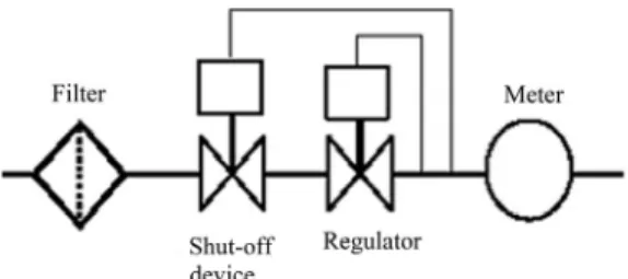
Gaz de France is involved in the importation, transmis-sion and distribution of natural gas throughout France. To perform these tasks, the Research and Development Division works on the improvement of all the technical systems used along the gas chain: from gas extraction and transmission to the consumer end-user. From the transmission natural gas network to gas customers appli-ances, the pressure is decreased in several steps by Pres-sure Regulating Stations (Figure 1).

The main functions of these systems are:  to decrease and control the pressure  to meter gas volumes

 to protect the outlet network against overpressure The first function is performed by a pressure regulator, the second one by a meter and the last one by shut-off and/or relief valves.

Although the technology and physical phenomena at work in regulators are fairly well known in terms of static performance, regulators are sometimes affected by operating instabilities [1,2] which can generate serious problems for operators: metering perturbation, shut-off devices closing or relief valves opening [3,4]. The pres-sure regulators are reliable enough to maintain a stable pressure level in steady conditions. However, in some specific configurations, some instabilities are observed

downstream of the pressure regulator: the downstream pressure is not properly controlled and oscillates around the set point with very high amplitude. This phenomenon is called “pumping”. When such problems occur, opera-tors have to go to the pressure regulating station, diag-nose the situation and search for a solution by applying empirical rules, which can be different from case to case. Several studies were carried out in the past in order to characterise the behaviour of regulators [5-7]. However, the conclusions were not easy to transmit to operators and difficult to generalise to the large number of devices used in the field. The study presented in this paper aims to provide mathematical models and experimental analy- sis for a common pilot controlled regulator. Both numerical simulations and experimental measurements have been carried out to predict the behaviour of this pilot

(3)

controlled regulator and to determine the operating con-ditions that avoid instabilities.

Computer simulation results are compared with ex-perimental measurements to provide validation guarantee validity of the mathematical model. Furthermore, the model will help to generalise the conclusions of this study to the most frequent regulators in the field.

2. Experimental Method

The experimental approach consists of extracting a pilot controlled regulator to install it on a test bench and to make it undergo a whole series of requests in order to determine the influence of several geometrical parame-ters or adjustments on the oscillations of the downstream pressure. To plan the tests and interpret the results, the method of experimental designs [8,9] was used.

2.1. Pilot Controlled Regulator Design

A regulator consists of a controlled valve, here a mov-able plug, which is positioned in the flow path to restrict the flow. The controlled valve is driven by an actuator: a diaphragm, dividing a casing into two chambers, provid-ing the thrust to move the controlled valve. One chamber is connected to the downstream volume through a sens-ing line and the pressure induced force exerted on the diaphragm is balanced by the set value of the down-stream pressure.

Pilot controlled regulators work pneumatically with

power autonomy and there are regulators in which the net force required to move the actuator is supplied by a pilot. The thrust is balanced by a controlled pressure: in this example, the auxiliary pressure (Pam) set in the lower casing (Figure 2).

Thus, a pilot controlled regulator is composed of:  a controlled valve: The movable part of the regulator

which is positioned in the flow path to restrict the flow through the regulator,

 an actuator: The mechanism that makes the controlled valve move depending on the pressure in the two chambers,

 a pilot: its role is to compare the downstream pressure (Pa) communicated to it by the sensing line. It oper-ates on the main regulator by using the auxiliary pressure (Pam) which makes the actuator move in the desired direction,

 a pilot supply regulator: its role is to make the regula-tion independent from the upstream pressure and to provide a constant driving pressure (Pmc),

 an actuator case: The house of the actuator. When the pressure in each chamber is different from atmos-pheric pressure, the chamber at the highest pressure is called the “motorized chamber”,

 reject and sensing line: The lines that connect impulse points to the regulator. The line with no internal flow is called the “sensing line”; the one with an internal flow rate is called the “reject line”.

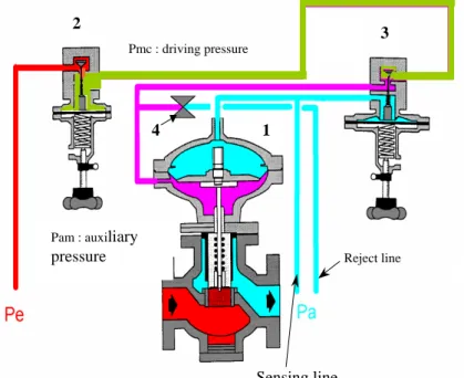
Figure 2. Schematic of pilot controlled regulator (1: main regulator, 2: pilot supply regulator, 3: pilot, 4: creeper valve).

Reject line Sensing line Pmc : driving pressure 2 3 1 4

Pam : auxiliary pressure

(4)

the pilot. In fact, prior to the pilot, another direct acting regulator, the pilot supply regulator, prevents upstream disturbances by reducing the upstream pressure down to the motorizing pilot pressure (Pmc) (Figure 2).

To sum up, a pilot controlled regulator is composed of three regulators: the main regulator, the pilot and the pilot supply regulator. It is also fitted out with several sensing lines and a valve which called the pilot restrictor. This restrains the flow between the pilot regulator and the downstream pipe.

2.2. Experimental Set-Up

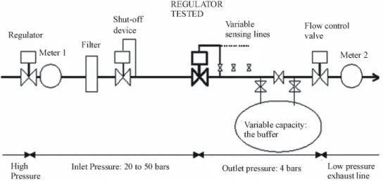
The regulators in test are devices with a nominal diame-ter of 50 mm. The test bench is able to reproduce the real working conditions of the regulator (flow-rate up to 10000 m3 (n)/h—inlet pressure up to Pe = 50 bars —outlet pressure controlled at Pa = 4 bars). Basically the arrangement consists of a first regulator located upstream which controls the inlet pressure, then the regulator being tested, and finally a piping system that enables provision of a variable capacity of the downstream buffer con-nected to a flow control valve that settles the load flow rate (Figure 3).

2.3. Experimental Tests

A test is done in two steps. The first step called initialisa-tion, consists of opening the flow control valve gradu-ally until the pressure downstream and the constant driv-ing pressure (for a pilot controlled regulator) reach their set point. At the end of initialisation, the flow obtained is almost established.

After having fixed all the parameters on the bench (flow rate, inlet and outlet pressure, buffer size, length of the sensing lines, the driving pressure, opening of pilot restrictor), having reached their set point and having

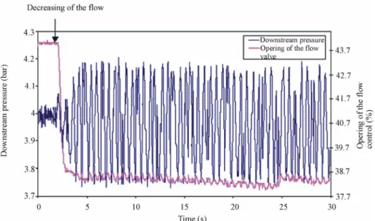
brought the regulator to stable operating conditions, we create a disturbance which consists of decreasing the flow rate of 1000 m3 (n)/h in a short time in order to trig-ger pressure oscillations. As shown in Figure 4, the test consists of recording and observing the oscillations of the downstream pressure. The amplitude and frequency of oscillations depend on all these parameters. The influ-ence of all of them has to be studied, but to limit the number of tests; we applied an experimental design ap-proach.

3. The Numerical Approach

The second part of the study consisted of developing an analytical model. It was considered that a better under-standing of the physical phenomena involved is an ap-propriate method to define the operating conditions that maintain a suitable level of pressure for the regulator tested and then to extend the conclusions to any regula-tor. The physical model of a pilot controlled regulator requires several approximations that will have to be va- lidated by comparisons of simulations and measure-ments.

The modelling of the gas behaviour with the different components of the regulator is quite complex because the physical phenomena involved (turbulence, compressibil-ity, fluid-structure interactions, unsteadiness, etc.) remain challenges for numerical simulation. The applied model-ling corresponds to the usual approach. It consists in breaking down the system to a set of subsystems reduced to their essential behaviours, making assumptions, proximations and mixing empirical and analytical ap-proaches. At the lower level, the main subsystems are:  the fluid systems

 the solid mechanical elements of the regulator itself  the flow through the valves

Figure 3. Test bench.

(5)

Figure 4. Downstream pressure following the reduction of the flow rate.

3.1. Generic Equations of the Hydraulic Models

Very few publications deal with the modelling of dy-namic gas systems [10]. Most studies in fluid mechanics concern stationary problems or are based on a linearized approach in the vicinity of a working point. These mod-els are not relevant to a gas pressure regulator since the flow direction in the process lines is likely to change at any time.

Thus, the usual pressure drop approach is not suffi-cient to simulate the oscillations which are partly due to the time delay induced by gas inertia in pipes and cham-bers. Only accounting for pressure drop and compressi-bility effects does not enable simulation of the oscilla-tions. The method for modelling flow in pipes is presented below.

The flow field is given by the flow velocity u, the pressure P, the density and the temperature T. The model is based on equations of the one-dimensional flow of a compressible, viscous, Newtonian fluid that are derived from the conservation of mass, momentum and energy completed with the equation of state [11].

Conservation of mass

The difference between the mass flow rate entering and leaving a control volume induces changes in density, this leads to the equation:





d d 0 d d u t x     

(1)

Conservation of momentum

The equation of motion is derived from Newton’s law. We consider here only the pressure and friction forces which act on the boundary of the fluid domain. The forces acting on the mass of fluid such as gravitational

effects are not taken into account. We then obtained the following simplified form of the Navier Stokes equa-tions:

 

d . d d S S S u _{u n u S} _{Pn S} _{n S} t  _ _       



d      

(2) This equation can also be written in local form:







2



2 d d d d d d 2 u u P _{u u} t x x D    _{ }         (3)

The first two terms represent the inertia of the gas, the third, pressure forces and the fourth, friction forces.

However:

D L

 _

and q. .u S (4) where  is estimated using the Idel’cik correlation [12]

Thus, for an element of cross sectional area S, and characteristic length L, and using the two previous Equa-tions (4), the generic equation of conservation of mo-mentum used for the hydraulic models is written in the form:





d 1 d 1 d d d d 2 q u q P u u S t S x x  L            (5) Conservation of energy

The energy balance can be written in a local formula-tion [13]: ij j i i i i i u u Pu e u t t x x  _i i x  _   _          

(6) This formulation completed with the balance of kinetic energy (the product of Equation (2) and velocity) yields:

(6)

j i i ij i i u e _u P t x x xi  _   _          

(7) Finally, introducing the enthalpy defined by

P e h    and dh de d P     _{  }   = CpdT + 1-T







dP

(8) Where β represents the coefficient of thermal expansion:

P 1 d = -dT         

(9) The general energy equation can then be written:

T T d Cp t x d i i i i u P u T i ij j x t x   _   _            

(10) The last term represents the contribution of viscous friction that has been neglected. In our first approach, the walls are adiabatic and the only conductive heat flux comes from both ends of the pipe. So, for one dimen-sional flow in an adiabatic pipe, the integral formulation of Equation (10) is then:





d d d Cp . d d out in d T T u S T t x  _  _       P t  (11) Equation of state

The above Equations do not give a complete descrip-tion of the modescrip-tion of a compressible gas. The reladescrip-tion- relation-ship between pressure variations and changes in tem-perature and density needs to be set through an equation of state. We used the usual form:

P _ZRT

 

(12)

R is the gas constant and Z the compressibility

coeffi-cient. The well known perfect-gas (Z = 1) approximation may not be suitable for this application since the pressure can vary quite widely between upstream and down-stream. For that reason the equation of state derived by Peng-Robinson [14] has been used:







 

3 2 2 2 3 1 3 2 Z  B Z  A B  B Z AB B B



0 With: 2 . . . a P A R T   and . . b P B R T  for T =0.7·Tc 2 2 2 0.45724 0.0778 c c c c T a R P T b R P       c

P , T_c: pressure and temperature of the critical point









2 2 0 10 1 0.37464 1.54226 0.26992 1 log 1 r c w w T P w P  _{ } _ _{ } _ _{ }        _ _   r c T T T 

3.2. Generic Equations of Mechanical Models

There are two different mechanical models for the three regulators. The same model is used for the pilot and the pilot supply governor, which are direct acting devices. In fact, the nature of the forces acting on the diaphragms of these regulators is identical: pressure force in upper cas-ing (the motorization chamber) and sprcas-ing stiffness in lower casing. The pre-stressed spring of the pilot gover-nor allows regulation of the pilot feed pressure whereas the characteristic of the pilot’s spring is modulated to adjust the downstream pressure. The approach is some-what different for the main regulator that integrates pres sure forces on both sides of the diaphragm.

Taking into account pressure forces, spring stiffness and damping the motion of the plug is driven by:



0



 

f

Mx  Ps K x x Mg F sign x   C x (14)

P denotes the pressure difference between both sides of the diaphragm, s is the diaphragm’s area, and F is the friction force resulting from the relative motion between the actuator and an O-ring seal (assumed to be Coulomb friction).

3.3. Generic Equations of Valve Models

There are two different models to represent the flow through the valves based on the pressure on both sides of the valve. The flow conditions vary widely whether sonic conditions are reached or not. The modelling for both sonic and subsonic valves are based on classical results and specific assumptions for a global approach. The model is based on established isentropic flow of a perfect gas. Following Liepmann and Roshko [15], the energy equation leads to:

1 2 1 2 1 1 1 1 2 1 P P u P             _ _{  }  _ _ _ _    

(15)

So assuming isentropic flow:

1 2 2 1 1 1 2 P P T T           _ _ _ _    

(16) and considering that the pressure loss is quite small

(7)

enable representation of the whole system, in particular the motions of actuators. To enable the treatment of Equations (1), (4) and (11), the pipe lengths have been separated using the following approximations for the gradients: 2 1 1 P P   , Equation (15) leads to 





* * 1 1 2 * 1 2 G G T q K P P P with K S T P    

₍₁₇₎ 2 1 d d d f f f x x  

(18) where S denotes the flow area at the plug; P*, T*, ρ*

re-spectively stand for the pressure, the temperature and the

density at the reference conditions. where dx represents the length of one piece and fi the

value of the function f at each end. The sonic conditions are reached at the plug if the

pressure downstream is lower than the critical pressure

Pk defined by:

This approach does not lead to a very accurate spatial distribution, but satisfactionly takes into account of the main fluid dynamic phenomena involved in gas pressure regulators. 1 1 2 1 k P P         _   

(18) Equation (13) can then be rewritten for sonic flow by

1 1 * * 1 1 * 1 n ' 2 2 1 1 G G q K P with K T S an T P             _  _   d q uS

₍₁₉₎

The algebraic-differential equations corresponding to the global model were solved by [17], whose specific feature is the possibility of formulating implicit equations dealing with discontinuities.

3.5. The Global Model

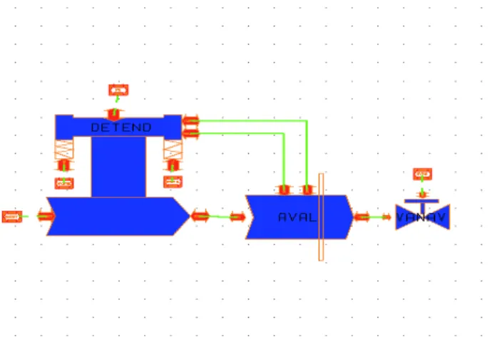
The global model is an assembly of three functional models (Figure 5) that represent: the downstream valve (VANAV), the downstream volume (AVAL) and the regulator itself (DETEND). The command statements are:

The values of the parameters KG and KG' depend

significantly on the shape of the plug which is usually quite complex. They had to be determined for each valve by experiments. In practice for natural gas, it is usually

considered that K_G' = KG/2.  Upstream pressure and temperature

 Setting of springs of the pilot and supply regulator

3.4. The Numerical Method _{ The opening of the downstream valve.}

The downstream valve is an elementary model that es-timates the flow rate as a function of the valve opening and the pressure in the downstream volume. The down-stream volume is an assembly of elementary models: pipes, junction points to connect to process lines. The pilot controlled regulator model (Figure 6) is a compli-cated hierarchical model gathering models for the pilot, the pilot supply governor, the main regulator, pipes, This modelling was performed with a general software

program [16], designed for the modelling and simulation of technical and dynamic systems.

This deals with algebraic differential equations and not with partial differential equations such as those derived in the set of Equation (1), (5) and (11) which would have required a Computed Fluid Dynamic (CFD) solver to be properly treated. However, a CFD approach does not

(8)

1 1 22 5 3 4 1 2 3 4 5

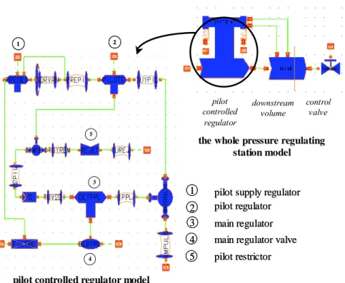
pilot supply regulator pilot regulator main regulator main regulator valve pilot restrictor 1 2 3 4 5

pilot supply regulator pilot regulator main regulator main regulator valve pilot restrictor

pilot controlled regulator model

pilot controlled regulator downstream volume flow control valve

the whole pressure regulating station model

Figure 6. Schematic of the pilot controlled regulator model.

chambers and valves: two different sonic valves for the main regulator and the pilot supply regulator, and two subsonic valves: one for the creeper valve and the other for the pilot regulator (Figure 6).

4. Application

Figure 7 shows a pilot controlled regulator. The up-stream pressure is expanded through a plug. It is com-posed of a pilot supply regulator whose role is to return the regulation quality independent of the upstream pres-sure and to provide the constant driving prespres-sure (Pmc). It is also composed of a pilot the role of which is to compare the downstream pressure (Pa), which is linked to it by the sensing line to the set point pressure, and ac-cording to the variation observed, it operates on the main regulator by using the auxiliary pressure (Pam), which moves the actuator in the desired direction.

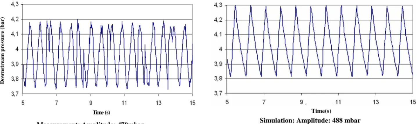
In order to validate the model of the regulator, the nu-merical results are compared to measurements on the test bench. It is generally noted that the numerical model reproduces, with a satisfaction level of accuracy, the os-cillations observed on the test bench (Figure 8).

4.1. Some Parametric Studies of Regulator Stability

It turned out from the complete study that the amplitudes of oscillations vary widely with some parameters, in par-ticular with downstream volume. They depend also on

the opening of the creeper valve and on the upstream pressure.

 Downstream volume effect

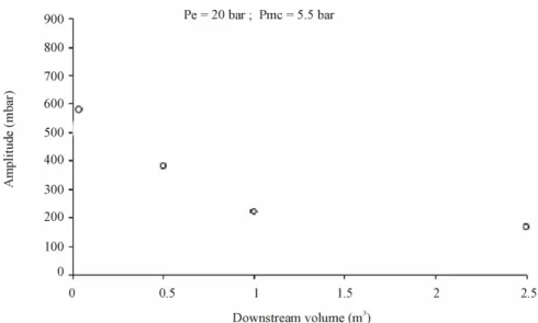
To study the effect of the downstream volume, we have fixed the other influence parameters (Pe = 20 bar, Pmc = 5.5 bar) and vary the downstream volume . The amplitudes and frequencies of oscillations are reduced for the highest downstream volume (Figure 9). Down-stream volume was increased by 0.04 m3 to 2.5 m3 and calculations as well as the tests showed that the size of downstream volume was important for small volumes. It is thus imperatively to avoid downstream volumes lower than 1 m3 for which the oscillations increase dramatically (about 600 mbar).

 Upstream pressure effect

According to Figure 10, an increase in upstream pres-sure (Pe) tends to raise the amplitudes of oscillations. This figure also gives a global illustration of the influ-ence of the driving pressure (Pmc) on the amplitudes and confirms that its effect is not very sensitive.

 Creeper valve effect

Another very important feature is the opening of the creeper valve. Three different openings of creeper valve have been tested: 0.25; 0.5 and 1 (turn) for four cases. Increasing the opening of the creeper valve for all the cases, raise slightly the amplitudes (Figure 11).

The other parameters considered have less influence on the regulator stability. For example the lengths of

(9)

Pmc Upstream pressure : Pe Pam Actuator Moving shift Spring Sensing

line _{Reject line}

Downstream pressure : Pa

Downstream pipe

Figure 7. Schematic of the pilot controlled regulator.

Figure 8. Simulation and measurement of downstream pressure for; V= 0.04 m3; Pe = 20 bar; q = 4000 m3/h.

Measurement: Amplitude: 470mbar Simulation: Amplitude: 488 mbar

Time (s) D o w n st rea m p ress u re ( b a r) Time(s)

(10)

Figure 9. Effect of the downstream volume on the amplitude of downstream pressure.

Figure 10. Effect of the upstream pressure on the amplitude of the downstream pressure.

Case Downstream volume: V (m3) Upstream pressure: Pe (bar) Driving pressure: Pmc (bar) Flow rate :q(m3(n)/h)

1 0.04 20 5.5 4000

2 2.5 20 5.5 4000

3 0.04 50 5.5 4000

4 2.5 50 5.5 4000

(11)

sensing lines, the opening of the antipumping valve. This feature has been confirmed by measurements and simu-lations.

5. Conclusions

The final objective of the study presented in this paper is to improve the process control of the pressure regulator that is to define the operating conditions that maintain a constant set pressure at small enough oscillations within tolerance field. For that purpose, numerical and experi-mental approaches have been performed.

The comparison of calculations and measurements, has confirmed the relevance of the modelling. From a quali-tative and a quantiquali-tative point of view, the calculations are in good agreement with experiments. Generally, the amplitude of oscillations increases dramatically for small volumes (V = 0.04 m3) and higher upstream pressure. As regards to the other parameters such as opening of creeper valve and driving pressure, their influence on the oscillation downstream pressure is not very sensitive.

Other adjustment parameters such as length of sensing lines or opening of the antipumping valve, have only marginal influences on the regulator stability.

6. Acknowledgments

The authors wish to express their indebtedness to Messrs. MODE Laurent and DELENNE Bruno of the Research and Development Division of Gaz De France for their contributions toward the success of this work.

REFERENCES

[1] H. W. Earney, “Causes and Cures of Regulator Instatbil-ity,” Fisher Controls International, Inc., Marshalltown, 1996.

[2] C. Carmichael, “Gas Regulators Work by Equalizing Opposing Forces,” Pipe Line & Gas Industry, 1996, pp 29-33.

[3] B. Delenne, L. Mode and M. Blaudez, “Modelling and Si- mulation of a Gas Pressure Regulator,” European

Simula-tion Symposium, Erlangen, Germany, 26-28 October 1999.

[4] B. Delenne and L. Mode, “Modelling and Simulation of Pressure Oscillations in a Gas Pressure Regulator,”

Pro-ceedings of American Society of Mechanical Engineers,

Vol. 7, Orlando, 2000.

[5] Association Technique de l’Industrie et du Gaz en France, Manuel pour le transport et la distribution du gaz, titre V “Détente et Regulation du Gaz,” 1990.

[6] K. J. Adou, “Etude du Fonctionnement Dynamique des Régulateurs-Detendeurs Industriels de Gaz,” Ph.D. Thesis, Université Paris VI, Paris, 1989.

[7] F. Favret, M. Jemmali, J. P. Cornil, F. Deneuve and J. P. Guiraud, “Stability of Distribution Network Governors

—R&D Forum Osaka Gas,” 1990.

[8] J. Goupy, “Plans D'expériences Pour Surface de Ré-ponse,” Dunod, Paris, 2000.

[9] J. Goupy, “La Méthode des Plans d'expériences: Optimi-sation du Choix des Essais et de L’interprétation des Résultats,” Dunod, Paris, 1988.

[10] J. P. Schlienger and E. Bordenave, “Ecoulement Insta-tionnaires de Gaz en Conduite,” 11 ème Congrès

Interna-tional du Gaz à Nantes, 1994.

[11] H. Schlichting, “Boundary Layer Theory,” McGraw Hill Book Company,Auckland, 1979.

[12] Idel'cik, “Spravotchnik po Guidravlitcheskim Soprotiv-leniam,” Memento des Pertes de charges, Gosenergoizdat, Moscow, 1960.

[13] J. Taine and J. P. Petit, “Transfert de Chaleur; Thermique; Ecoulement de Fluide,” Dunod, Paris, 1989.

[14] D. Y. Peng and D. B. Robinson, “A New Two-Constant Equation of State,”Industrial & Engineering Chemistry

Fundamentals, Vol. 15, No. 1, 1976, pp. 59-64. doi:10.1021/i160057a011

[15] H. W. Liepmann and A. Roshko, “Elements of Gas Dy-namics,” John Wiley and Sons Inc.,Hoboken, 1962. [16] A. Jeandel, F. Favret, L. Lapenu and E. Lariviere,

“ALLAN. Simulat Ion, a General Tool for Model De-scription and Simulation,”International Conference of

the International Building Performance Simulation Asso-ciation, Adlaide, 16-18 August 1993.

[17] M. Nakhlé, “NEPTUNIX an Efficient tool for Large Size Systems Simulations,” 2nd Internationnal Conference on

(12)

NOMENCLATURE

Cf viscous damping (kg/s)

Cp specific heat at constant pressure (J/K/kg)

F  Friction force (N)

D pipe diameter (m)

e specific internal energy (J/kg)

g gravity acceleration (m/s2)

h specific internal enthalpy (J/kg)