The Dimensional Model : a framework to distinguish spatial relationships

The Dimensional Model: a framework to

distinguish spatial relationships

Roland Billen, Siyka Zlatanova, Pierre Mathonet & Fabien Boniver

Roland Billen, MSc., Aspirant FNRS (Research Fellow), Geography Dept., University of Liege, allée du 6-Août 17, 4000 Liège, Belgium, +32-(0)4/3665752, +32-(0)4/36656 93, Roland.billen@ulg.ac.be

Siyka Zlatanova, Dr. Eng., Geodesy Dept., Delft University of Technology, Thijsseweg 11, 2629 JA Delft, The Netherlands, +31 (0)15 278 2714, +31 (0)15 278 2745, S.Zlatanova@citg.tudelft.nl

Pierre Mathonet, Dr. Sc., Math. Dept., University of Liege, grande traverse 12, 4000 Liège, Belgium, +32-(0)4/3669480, +32-(0)4/366 9547,

P.Mathonet@ulg.ac.be

Fabien Boniver, Dr. Sc., Aspirant FNRS (Research Fellow), Math. Dept., University of Liege, grande traverse 12, 4000 Liège, Belgium, +32-(0)4/3669417, +32-(0)4/366 9547, F.Boniver@ulg.ac.be

ABSTRACT

The particularity of GIS compared to other information systems is the management of spatial relationships, i.e. the connections or interrelations between real objects in the geometric domain. A number of frameworks use topology as basic mechanism to define spatial relationships. OpenGIS consortium has adopted one of them, i.e. the 9-intersection model. In this paper, a new framework for representing spatial relationships - the Dimensional model - is introduced. The model was first developed for convex spatial objects and is now extended to topological n-manifolds. It is based on two major concepts, i.e. the dimensional elements of spatial object and the dimensional relationships being the relationships existing between dimensional elements. It represents a very large group of spatial relationships and provides a flexible framework to consider either generalised or specialised types of relationships.

Keywords: spatial relationships, spatial model, convexity, topological manifolds.

1. Introduction

The development of a mathematical theory for categorising relationships has been identified as one of the most essential task to tackle the diversity and incompleteness of spatial-relationships’ representations (see Boyle et al. 1983, NCGIA 1989). Among all the approaches (e.g. metrics, topology, ordered sets), topology seems the most appreciated (see Egenhofer et al. 1994, Egenhofer 1989, Egenhoher and Sharif 1998, Clementini et al. 1993, Kainz et al. 1993, Molenaar 1998). OpenGIS consortium has adopted one of the topologically based frameworks, i.e. the 9-intersection model, as a generic mechanism for implementation and development.

In this paper, a new framework for representing spatial relationships named the Dimensional model (DM) is introduced. The model was first developed for convex

spatial objects and is now extended to topological n-manifolds. The paper is organised in the following sections. Firstly, the order’s concept for convex bodies is presented. Then, the order’s concept for a topological manifold is developed. A formal description of the Dimensional model follows. After a brief comparison with the 9-intersection model, some spatial relationships are depicted using DM. Finally, the implementation of the DM is overviewed.

2. An order formula for convex bodies

2.1. Affine subspaces and convex sets

Geographers and mathematicians use coordinates to describe location in space. Whenever, d is a positive integer, we denote by Rd the set of tuples (α1,...,αd) of real numbers α1,...,αd. As Euclidean vector (or affine) space, Rd is the natural

framework in which geometry can formally be studied. It is also the first example of Euclidean topological space. A detailed introduction to general topology and manifolds can be found in Alexandrov (1998) and Lee (2000).

A subset A of Rd is an affine subspace if, for any distinct points x, y belonging to A, the straight line defined by x and y lies in A. Points, straight lines, planes, and

R3 itself are the only affine subspace of R3. Their respective dimensions are 0, 1, 2 and 3. An affine subspace of dimension d-1 of Rd is named hyperplane. For instance the hyperplanes are merely straight lines in R2 and planes in R3. A hyperplane divides the whole space in two regions, called halfspaces.

A subset A of Rd is convex if, for any two points x,y belonging to A, the segment [x,y] lies in A.

A supporting hyperplane M of a convex set C is a hyperplane such that - C is included in one of the halfspaces defined by M,

-

M

∩C

≠

∅.

Figure 1 shows examples of convex sets and supporting hyperplanes in R2 and R3.

Figure 1: Examples of closed convex sets and hyperplanes 2.2. Order of points in closed convex set

Let C be a convex set, closed with respect to the Euclidean topology. Each point of C has an order, whose definition is given in Berger (1978, p. 50), and can be stated as follow.

Let C be a closed convex set in Rd and

x

∈

C

. The order of x in C, denoted by o(x,C), is the dimension of the intersection of all supporting hyperplanes containing x.

In particular, if no supporting hyperplanes contains x, then x has order d. One can prove that those points with order d are exactly the interior points of C with respect to the Euclidean topology.

Figure 2 shows points with various orders in a triangle, a drop, and a segment. For instance, the top point of the triangle has order 0. Indeed, infinitely many supporting hyperplanes (only two are represented) go through it and intersect in that point itself.Figure 3 shows examples in R3.

Figure 2: Order of points of closed convex sets in R2 (with some hyperplanes)

Figure 3: Order of points of closed convex sets in R3 (without hyperplanes)

3. An order formula for manifolds

More often than not, objects that one deals with in GIS applications are not convex. It is then natural to seek for a suitable formula for more general objects. Those will be topological manifolds. Our approach goes as follow: given a point x in a topological manifold, we create a closed convex neighbourhood of x and compute its order with respect to this neighbourhood. The key point is that, intuitively, the order of a point is a “local” property: it actually depends only on the manifold in a neighbourhood of x

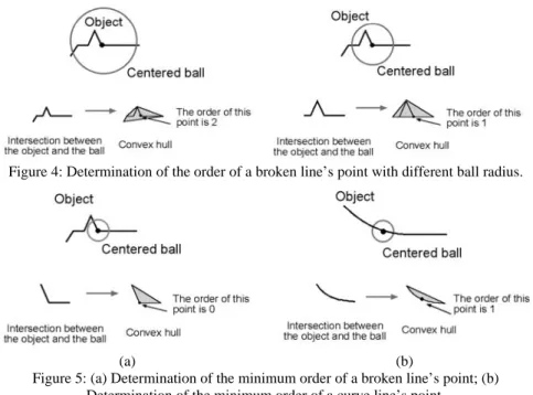
Therefore, the steps to find the order of points are: 1) determine if the point of interest stands on the interior or the boundary of the manifold; 2) centre a ball on this point with a given radius r; 3) take the intersection between the ball and either the manifold or the boundary of the manifold; 4) determine the convex hull of this intersection; 5) determine the order of the point regarding the convex object created (the convex hull); 6) repeat the operation 2 to 6 with a smaller radius, until getting a minimum value for the order.

3.1. Topological manifolds

Let n be a positive integer. We denote by Rn+ the subset of tuples (α1,...,αn) with

αn

≥

0

.. A subset A of Rd is a topological n-manifold with boundary if each point

has neighbourhood which is homeomorphic to an open subset of R

A

x

∈

n

+.

Let A be such n-manifold. It is the disjoint union of its interior,

A

°

,

and its boundary,

∂

A

.The points belonging to

A

°

are named interior points. A point is

interior if it has a neighbourhood homeomorphic to an open subset of Rn. It is worth noticing that those definitions do not coincide with the Euclidean topological definitions of interior and boundary.

Two additional notations will be useful. If B is a subset of Rd, we denote by conv(B) the convex hull of B, which is the smallest convex subset of Rd containing B. If r is a positive real number and

x

∈

Rd, we denote by bx,r the closed ball with centre x and radius r.

3.2. The general formula

We can now write the general formula that encapsulates the algorithm presented above. Let X be a topological manifold. Assume furthermore that X is closed as a subset of Rd. If x is an interior point of X, then its order is defined as:

))

(

,

(

lim

, 0 , 0r

o

x

conv

b

xr

X

r→ ≠

∩

. (1)

Now, if

x

∈

∂

X

, then its order is:

))

(

,

(

lim

, 0 , 0r

o

x

conv

b

xr

X

r→ ≠

∩

∂

. (2)

In both cases, the limit exists and equals the minimum of the values of the function o.

Figure 4 illustrates this approach for 1-manifold. Figure 5 and 6 show some more examples for 1-manifold (curve line) and 2-manifold.

Figure 4: Determination of the order of a broken line’s point with different ball radius.

(a) (b) Figure 5: (a) Determination of the minimum order of a broken line’s point; (b)

(a) (b) Figure 6: (a) Determination of the minimum order of a polygon’s boundary point; (b)

Determination of the minimum order of a polygon’s interior point.

4. The Dimensional Model (DM)

The Dimensional model is a framework to describe both spatial objects and spatial relationships. The spatial objects are composed by dimensional elements, which are based on order’s points of object. The spatial relationships between spatial objects are described in terms of dimensional relationships, i.e. relationships that exist between the dimensional elements of the objects.

4.1. Spatial objects in DM

In our model, a simple spatial object of dimension d is equivalent to a topological d-manifold. They are called simple because it is possible to apply directly the order formula to them, and therefore determine their dimensional elements. We also define a complex spatial object (as a combination of simple spatial object), which will not be discussed here (see Figure 7).

Simple spatial objects (manifold) Complex spatial objects (aggregation of simple objects)

Figure 7: Examples of spatial objects

4.2. Dimensional elements of DM

The dimensional elements are associated with different parts (or points) of a spatial object according to their order.

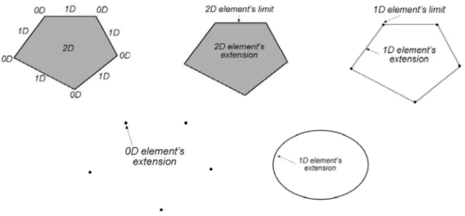
The α−dimensional element (denoted αD-element) of a spatial object C (which has at least dimension α), corresponds to the set of all the points (or parts) of C which have order 0 to α.

The αD-element of a spatial object C has an extension and may have a limit. The extension is the subset of C formed by its points of order α, and the limit is the subset of C formed by its points of order 0 to order (α-1).

Thus, if the αD-element has a limit, this limit corresponds to a lower (α-1)D-element. The 0D-element does not have a limit by definition. Figure 8 illustrates the dimensional elements of a polygon. First, the order of all the points is determined. This convex is composed by a 2D-element, a 1D-element and a 0D-element. The different extension and limits are presented in the figure 8. In the case of an ellipse, the 1D-element does not have a limit. It should be noted that there is one and only one xD-element by object.

Figure 8: Order of points and dimensional elements of a polygon and of an ellipse 4.3. Dimensional relationships

The dimensional relationships are defined as the relationships existing between dimensional elements. These relationships can either be total, partial or non-existent, and are oriented (from one element to an other one).

A dimensional element is in total relation with another dimensional element if their intersection is equal to the first element, and if the intersection between their extensions is not empty.

A dimensional element is in partial relation with another dimensional element if their intersection is not equal to the first element, and if the intersection between their extensions is not empty.

A dimensional element is in no relation (non-existent) with another dimensional element if the intersection between their extensions is empty.

Figure 9 illustrates the three types of dimensional relationships for 2D-elements.

No relation (non-existent) Total relation Partial relation Figure 9: The different types of dimensional relationships between two 2D-elements (from

4.4. The Dimensional model for investigation of spatial relationships

The dimensional elements (with their limits and extensions) and the dimensional relationships (i.e. total, partial and non-existent) are the basic tools to decode spatial relationships. The spatial relationship between two objects can be expressed by the dimensional relationships that exist between the dimensional elements of both objects. For example, let’s consider a polygon A (with 2D, 1D, 0D elements) and a line B (with 1D and 0D-elements). The dimensional relationships between the spatial objects A and the spatial object B can be identified in the following sequence: first, check the dimensional relationship between 2D-element of A and all the dimensional elements of spatial object B; then, check the dimensional relationship between 1D-element of A and all the dimensional elements of spatial object B, etc. The dimensional relationships between B and A can be found following the same approach. Three groups of dimensional relationships can be distinguished following this approach, i.e. the simplified, the basic and the extended relationships.

A dimensional relationship is coded using the notations R for relationships, nD for dimension of the element of the first object, and y dimension of the element of the second object. R2D1 represents the dimensional relationships between the 2D-element of the first object and the 1D-2D-element of the second object. Furthermore, a numeric code for the three types of dimensional relationships, i.e. 0 for non-existent, 1 for total and 2 for partial, is specified.

The basic relationships. This group contains all the relationships between every possible combination of dimensional elements. For example, the spatial relationship between a polygon (considering 2D, 1D, 0D elements) and a line (considering 1D and 0D elements) can be expressed by basic dimensional relationships as follows:

R2D1 R2D0 R1D1 R1D0 R0D1 R0D0 {0,1,2} {0,1,2} {0,1,2} {0,1,2} {0,1,2} {0,1,2}

where 0, 1, 2 correspond to the possible dimensional relationships, i.e. non-existent, total and partial.

The extended relationships. As it can be realised, the partial relation can be further investigated for the dimension of the intersection. For example, in R3, a 2D-element and a 1D-2D-element may have a 1D- or a 0D-intersection. If the intersection has the same dimension as the lowest dimensional element in the relation, it keeps the code 2 (e.g., if a 2D-element and a 1D-element have a 1D-intersection, it would be noted as R2D1 2). If the dimension of the intersection is just inferior, then it would have code 3 (a 0D-intersection in the example, R2D1 3). Our example of spatial relationships between a polygon and a line becomes:

R2D1 R2D0 R1D1 R1D0 R0D1 R0D0 {0,1,2,3} {0,1,2} {0,1,2,3} {0,1,2} {0,1,2} {0,1,2}

The simplified dimensional relationships. In many cases the dimensional elements of the second object is not relevant. For example, it might be interesting to know if the 2D-element of a polygon has a relationship with another object independently

of its dimensional elements. In such cases, some dimensional relationships can be aggregated. The complete aggregation rules will not be exposed here. Our example becomes:

R2D R1D R0D

{0,1,2} {0,1,2} {0,1,2}

Figure 10 illustrates how the spatial relationships between a polygon and a line are represented according to the different groups in the Dimensional model.

Basic relationships R2D1 |R2D0 |R1D1 |R1D0 |R0D1 |R0D0 2 |0 |0 |0 |0 |0 Extended relationships R2D1 |R2D0 |R1D1 |R1D0 |R0D1 |R0D0 3 |0 |0 |0 |0 |0 Simplified relationships R2D |R1D |R0D 2 |0 |0

Figure 10: The Dimensional model applied to the relationship between polygon and line

5. The dimensional model versus the 9-intersection model

As mentioned, the 9-intersection model is a one of the topological relationships standard. We want to clearly expose the difference that exists between the 9-intersection model and the Dimensional model.

5.1. The 9-intersection model (9i model)

The framework is based on the assumptions of spatial objects (represented by 0,1,2,3-cells) without holes and intersecting parts. If the spatial objects A and B are defined in the same topological space, their boundary, interior and exterior are denoted by

∂

A

,

A

°

,

A

−

,

∂

B

,

B

°

and

B

−(see Egenhofer, M. and J. Herring, 1990). The binary relationship R(A,B) between the two objects is then identified by composing all the possible set intersections of the six topological primitives, i.e.

∂

A

∩

∂

B

,

A

° B

∩

°

,

∂

A

∩

B

°

,

A

°

∩

∂

B

,A−∩ B−, ,

, and , and detecting empty (0) or non-empty (1)

intersections. For example, if two objects have a common boundary, the intersection between the boundaries is non-empty, i.e.

B

A

−

∩

∂

A

−

∩

B

°

−

∩

∂

A

B

A

° B

∩

−

1

=

∂

∩

∂

A

B

; if they have intersecting interiors, then the intersection A° B∩ °is not empty, i.e.

A

° B

∩

°

=

1

. To represent the relationships a decimal coding is adopted here (see Kufoniyi 1995). That is to say that the binary number (obtained from a particular ordering of all the intersection) is converted into a decimal number. For example, the relationship that has a binary number 000011111 (considering the

ordering given above) equals decimal number 31 and hence the relationship is R031 (disjoint). Thus, all the decimal codes are between R000 and R512

5.2. Differences between 9i model and DM

The differences between the 9-intersection model and DM can be summarised as follows:

1. The definition space of 9i model is topological when it is affine one for DM. 2. In the 9i model, the spatial relationships are determined looking to

intersections of the topological primitives. In the DM, the spatial relationships are determined looking to intersections of the dimensional elements.

3. The 9i model is related to the cell approach. The dimension of the cells are not (always) equivalent to order of points (see Figure 11). Therefore, the union of d-cells of an object is not equivalent to its dD element, except for some special types of objects (as polytopes).

Object A Object B

Figure 11: Examples of differences between cell decomposition and dimensional elements.

4. The DM allows grouping spatial relationships at different level of complexity: more general groups than with 9i model, same kind of groups or more specific ones (see the next section).

6. Possible spatial relationships

As mentioned, three groups of dimensional relationships can be used to express the spatial relationship between objects. Furthermore, one has the choice to take into consideration only relevant dimensional element in a geographical perspective. For example, a particular geographical phenomena represented by a polygon may not need a distinction between the 1D-element and the 0D-element which form its border. In such a case, even though the 0D-element exists in the object’s definition, it would not be taken into account in the determination of spatial relationship.

The number of potential relationships between two objects depends, with respect to the Dimensional model, on: 1) the dimensional nature of the objects (given by dimensional elements), 2) the semantic dimension of the object (only the “relevant” dimensional elements from a semantic point of view) and 3) the group of dimensional relationships. Similarly to the 9-intersection model, only a small number of the theoretical relationships can be realised in reality (see Zlatanova, 2000 for examples in R3). The same approach is adopted, i.e. elimination of impossible relationships by negative conditions. All the possible relationships between line-line, line-surface, line-body, surface-surface, surface-body and finally body-body have been established and studied for the different criterion mentioned above. Note that in this study, some elements have been simplified, for

example the 0D of a line correspond only to its extremities (no broken lines). Table 1 portrays simplified, basic and extended relationships for all levels of dimensional relevancy.

Table 1: Possible relationships according to the Dimensional model

D el. Dim. Rel. Line- Line Surface- line Body- body Surface-surface Body- Line Body-surface S. 5 3 5 5 3 3 B. 5 3 5 5 3 3 (n)D E. 7 5 5 11 3 3 S. 11 10 8 15 6 8 B. 33 31 8 43 19 19 (n)D &(n-1)D E. 61 ? 15 ? 43 48 S. ? ? ? 19 ? B. ? ? ? ? ? (n)D &(n-1)D &(n-2)D E. ? ? ? ? ? S. ? ? ? B. ? ? ? (n)D &(n-1)D &(n-2)D &(n-3)D E. ? ? ?

With D el. = D element; Dim. Rel. = Dimensional relationship; S. = simplified; B. = basic; E. =extended

? non determinated

impossible case

33 possible relationships according to the 9-intersection model

Considering the highest and the second highest dimensional element and using basic relationship, the relationships reported by Zlatanova (2000) are exactly found. They are given in bolt font the table 1 (smooth grey). Most of the topologically equivalence cases can be “clarified” using some of the more complex criterions in the Dimensional model (i.e. everything that is below the shaded line in the table 1). Furthermore, more aggregated relationships can be found with simpler criterions (i.e. everything that is above this line). Figure 12 present the extended dimensional solutions (0D elements are not taken into account) to the topological equivalence R095 and R287 (between a body A and a surface B). R3D2 R3D1 R2D2 R2D1 R1D2 R1D1 (a) 0 0 2 0 2 0 (b) 0 0 0 0 2 0 (c) 0 0 0 2 0 0 (d) 0 0 0 0 0 2

Figure 12: Dimensional relationships for topological equivalence R095 (a and b) and R287 (c and d)

Another interesting example concerns the “meet” relationship between two bodies. All the spatial situations in Figure 13 are equivalent to R287 according to the 9-intersection model, while all of them can be differentiated with the Dimensional model. Solutions are given only for case a, b, c and d. The cases e and f need to take 0D-element into consideration.

R3D3 R3D2 R3D1 R2D3 R2D2 R2D1 R1D3 R1D2 R1D1

(a) 0 0 0 0 2 2 0 0 0

(b) 0 0 0 0 2 2 0 0 2

(c) 0 0 0 0 0 0 0 2 2

(d) 0 0 0 0 0 0 0 0 2

Figure 13: Dimensional relationships for topological equivalence (R287)

7. Implementation of the DM

The DM is spatial relationships oriented. However, it is possible to use it to enrich spatial data structures. Some convenient tests have been done. The “purest” solution is to use D elements instead of topological primitives. But of course some problems may occur when objects are transformed – the D elements are not invariant through all the homeomorphic transformations. A more pragmatic solution is to keep a topological data structure and compute the dimensional elements during the determination process of dimensional relationships. This computation uses colinearity and coplanearity algorithms. The search for an adapted implementation of DM has reach some very interesting concepts, such as the possibility to give up the single-valued map approach (see Molenaar, 1998). This is still under research and will not be developed here.

8. Conclusions

In this paper, we have presented a new framework, i.e. the Dimensional model, to distinguish spatial relationships of spatial objects. The Dimensional model allows representing a very large group of spatial relationships. It gives a flexible framework that allows either generalised or specialised types of relationships to be considered. The freedom in choosing geographically relevant dimensional elements and groups of dimensional relationships allows deciding on a particular complexity of spatial relationships. It covers a large range of spatial objects (topological n-manifold for simple spatial objects, and combinations of simple spatial objects for complex spatial objects).

Acknowledgements

The authors would like to thank Bernard Cornélis for his critical proof reading and constructive comments.

References

Alexandrov PS (1998), Combinatorial topology, Vol. 1, 2 and 3. Dover Publications Inc., Mineola, New York

Boyle A, Dangermond J, Marble D, Simonett D, Smith L and Tomlinson R (1983), Final report of a conference on the review and synthesis of problems and directions for large scale geographic information system development. Technical report, NASA NAS2-11246

Berger M (1978), Géométrie 3 : convexes et polytopes, polyèdres réguliers, aires et volumes. Paris, Cedic/Fernand Nathan

Clementini E, di Felice P and van Oosterom P (1993), A small set of formal topological relations suitable for end-user interaction, In: Proceedings of the 3th International Symposium on Large Spatial Databases. Berlin, Springer-Verlag, pp. 277-295

Egenhofer M (1989), A formal definition of binary topological relationships, In: Proceedings of the 3th International Conference on Foundation of Data Organisation and Algorithms, pp 457-472.

Egenhofer M, Clementini E and di Felice P (1994), Topological relations between regions with holes, International Journal of Geographical Information Systems 8(2), pp. 129-144

Egenhofer M and Herring J (1990), A mathematical framework for the definition of topological relationships, In: Proceedings of Fourth International Symposium on Spatial Data Handling. Zurich, Switzerland, pp. 803-813 Egenhofer M and Shariff B (1998), Metric details for natural-language spatial

relations. ACM transactions on information systems 16(4), pp. 295-321 Kainz W, Egenhofer M and Greasley (1993), Modelling spatial relations and

operations with partially ordered sets, International Journal of Geographical Information Systems 7(3), pp. 215-229

Kufoniyi O (1995), Spatial coincidence modelling, automated database updating and data consistency in vector GIS. Ph.D. Thesis, ITC, The Netherlands Lee J (2000), Introduction to topological manifolds. New-York, Springer-Verlag Molenaar M (1998), An introduction to the theory of spatial objects modelling.

London, Taylor&Francis

NCGIA (1989), The research plan of the National Center for Geographic Information and Analysis. International Journal of Geographical Information Systems 3(2), pp. 117-113

Zlatanova S (2000), On 3D topological relationships, In: Proceedings of the 11th International workshop on Database and Expert System applications. Greenwich, London, pp. 913-919