Comparing predictive accuracy of real estate
pricing models:
an applied study for the city of Montreal
par
Simon P. Leblond
D´
epartement de Sciences ´
Economiques
Facult´
es des Arts et Sciences
Universit´
e de Montr´
eal
Travail de recherche pr´
esent´
e `
a M. William McCausland
en vue de l’obtention du grade de M.Sc.
en Sciences ´
Economiques
option ´
econom´
etrie
D´
ecembre 2004
c
Abstract
The object of this paper is to compare valuation methods for real estate in the context of automated mass valuation. Empirical tests are performed for the market of single family housing in the city of Montreal using several different specifica-tion. In- and out-of-sample predictions are compared using both transaction and appraisal data. Models studied include basic parametric hedonic price models, their spatial counterparts and the city’s assessment. Different issues are briefly addressed throughout the paper, including spatial dependence, effect of missing or incomplete data and assessment bias. Results show that spatial models outperform non-spatial ones. No model seems however to offer sufficient precision for automated mass val-uation.
Remerciements
Je dois souligner le soutient financier du CRSH qui m’a octroy´e une bourse de recherche de maˆıtrise et remercier la Chambre Immobili`ere du Grand Montr´eal qui m’a donn´e acc`es au donn´ees de transactions immobili`eres.
Ce travail repr´esente une ´etape importante de mon cheminement personnel, puisqu’il est le dernier morceau de mes 18 ann´ees d’´etudes. Plusieurs personnes doivent donc ˆetre remerci´ees pour m’avoir permis de me rendre jusqu’ici. Merci `a
´
Emilie, Vincent, J-C, Ol, Thalie et tous ceux qui ont su m’endurer chaque fois que j’ai exprim´e mon impatience lors de mes ´etudes. Un merci particulier `a ma m`ere et mon p`ere pour m’avoir ´epaul´e depuis le d´ebut et avoir ´et´e pr´esent pour relire mes travaux du premier au dernier.
Un gros merci `a mes professeurs du D´epartement qui m’ont inculqu´e ce que je sais aujourd’hui en ´economique, tout particuli`erement Fran¸cois Vaillancourt et Bill McCausland. J’esp`ere ne pas avoir trop abus´e de leur patience. . .
Finalement, merci `a mon grand-p`ere Leblond, Bon-Papa, pour m’avoir trac´e le chemin et ˆetre une source d’inspiration in´epuisable dans tous les aspects de ma vie.
1
Introduction
Real estate is a very important market in every country in the world. In Canada, the resale market alone represented a volume of over 164 billions dollars in 2000, while total real estate assets were worth over 1 trillion dollars in 2002 1. It is thus no wonder that real estate research has not only considerable academic appeal, but also large economic potential. Real estate pricing is one such area of research with great economic importance. Indeed, providing fair market values for properties is of importance for public assessors, banks, buyers and sellers, investors and many more. Traditional appraisal by a private firm is conducted by Direct Capital Comparison (DCC) and costs between 300$ and 1000$ for a owner-occupied house. Yet, even with all of this pecuniary incentive, automated alternatives to DCC have failed to penetrate professional practice for lack of accuracy (Jenkins & al., 1999).
Hedonic modeling is one of the alternatives used to estimate fair market value of houses and the one with the longest pedigree, appearing in the economic literature several decades ago in such work as Rosen (1974) and Palmquist (1980). The hedonic pricing method is used to estimate economic value for services or characteristics that directly affect market prices of a good. By looking at the price variations of the good when a characteristic changes we can thus put a value on that particular trait (King & Mazzotta, 2004)2. Even though housing is by far the most common application of the hedonic pricing method, it has been used to value a wide variety of items. Recent examples include video game characters traits (Castranova, 2004) and quality of opals (Cornelius, 1996).
In the housing context, the hedonic approach assumes a relation between market value for sold properties and a particular set of housing characteristics. This relation can then be used to predict market value of unsold properties with known attributes.
1All dollars mentioned in this report are Canadian dollars, 1 CAD ≈ 0.80 USD.
2A full discussion of the hedonic method and its critical assumptions can be found in Palmquist
However, hedonic pricing models are plagued by a number of problems and are unusable in a commercial way (Jenkins & al., 1999; Clapp, 2003; Lesage & Pace, 2004). This paper addresses two of these problems in the context of automated mass valuation for the housing market of Montreal: spatial dependence and the effect of missing or incomplete data. The objective is to test in- and out-of-sample different models that address these problems and compare them to a basic hedonic linear function and to the city’s valuation scheme. The question of assessment bias is also briefly discussed.
1.1
Automated mass valuation
Automated mass valuation3 applications include a city’s tax assessment or
nation-wide mortgage lending decision (Clapp, 2003). In these contexts, individual ap-praisal is infeasible or highly costly while it is still essential to have exact estimates of property prices. Here, we will compare the mass valuation that was done by the city of Montreal in 2003 to the performance of other hedonic valuation models taken in the literature.
The city’s assessment office performs assessments in a uniform way every three years for the whole island of Montreal. Even though this methodology is an im-provement over non-uniform practice used in other cities, the main problems of mass valuation remain: no attention can be given to individual properties and, so, the possibility of being incorrect is very high (Kay, 1990). Hyman (1998) even describes the practice as an “art” rather than a science. Results in the literature confirm that property tax assessment in general is plagued with inconsistent valuation (Cornia & Slade, 2003).
This author’s observation and belief for the case of Montreal is that tax
assess-3For the remainder of the text, “mass valuation” and “automated valuation” will be used as
ment systematically and significantly lags actual market prices. This downward “assessment bias” is observed by a number of studies for other real estate markets. Cornia and Slade (2003) find that the “assessed values are significantly lower than the respective sales prices” for Maricopa County (AZ). They also note that while assessed values increased between 3 and 5% over five years, market price increased over 30% for the same period. Many papers mention a temporal lag bias in ap-praisals or “appraisal smoothing” for both individual and mass valuation (Quan and Quigley, 1991; Clayton & al., 2001; Hansz & Diaz III, 2001; Baum & al., 2002). Goolsby (1997), who finds consistent assessor bias for many classes of single family homes in Washington State, suggests that underassessment may come from fiscal pressure: owners complain only when their properties are overassessed. Cornia and Slade (2003) mention that to avoid this problem, many tax assessors reduce by a certain coefficient the actual assessment (82% in their case).
Using sales from the fourth quarter of 2003 as our benchmark for market value, we will proceed to compare both the city’s appraised values and forecast from our hedonic models. Of course, useful information could be gained if the city’s assess-ment were not biased or could be used as an effective proxy for the fair market value.
1.2
Spatial dependence
Towards the end of the 80’s, Dubin (1988) introduced the notion of spatial auto-correlation4 in real estate. Since then, both spatial statistics and their applications
to real estate have received considerable attention (Anselin, 2002). Three reasons are usually invoked for the presence of autocorrelation in house prices. First, as is well known, house value depends on distance to various amenities (public transport,
4“Spatial dependence”, “spatial autocorrelation” and “spatial interaction” are synonyms which
city center, etc.). It follows that neighboring houses should be affected in a similar way by locational attributes. Second, neighborhoods are usually developed at the same time, so houses in a given neighborhood tend to be similar, sharing many characteristics (architecture, size, etc.). Finally, they share common public services (schools, fire stations, etc.) (Basu & Thibodeau, 1998; Militino & al., 2004). Not to account for spatial autocorrelation, if present, would yield inefficient parameters estimates and incorrect confidence intervals for predicted price values. Indeed, spa-tially autocorrelated residuals of a simple hedonic model violate the independence assumption of OLS in the same way temporal autocorrelation does. Modeling spa-tial dependence in housing data sets has thus been a major subject of the real estate literature for the past decade both for the sake of efficiency and for the great predic-tive improvement it showed over simple OLS estimation of hedonic functions (Pace & al, 1998; Dubin, 1998; Clapp, 2003).
While many spatial specification have been considered in recent years (see Case & al., 2004 or Militino & al., 2004 for examples), basic specifications described in text books by Anselin (1988) and Cressie (1993) are still predominantly being used in empirical studies to model spatial autocorrelation (Anselin, 2002). These models rely on “spatial lags” of either the dependent variable, the errors or the independent variables. The first two are analogues of their time series counterpart: spatial autoregressive (SAR) with autoregressive models and spatial moving average (SMA) with moving average models5. A mixed model, the mixed regressive spatial
autoregressive model with spatial autoregressive disturbance (or SARMA for short), also exists which mimics the time-series ARMA model for spatial data.
In this paper, diagnostic tests described in Anselin & al. (1996) are performed on our basic hedonic model estimated by OLS to test for spatial interaction. The
5Names of the models vary throughout the literature. Lesage (1999), for instance, talks of
spatial error model (SEM) instead of SMA and SAC in place of SARMA. For simplicity’s sake, we stick with the variation of the time-series names
three basic models described in the previous paragraph (spatial lag of the dependent variables, SAR and SMA) are then used to model and capture spatial dependence.
1.3
Missing data
Real estate empirical research is faced with the obstacle of obtaining reliable data. Most real estate databases include one or more data irregularities: missing data, censoring or truncation, measurement error, etc. (Knight & al., 1998) For the MLS database, missing data is indeed a problem: over 50% of transactions of interest suffer from one or many missing data fields. Knight & al. (1998) lists three con-ventional solutions to the problem: 1. eliminate from the data set those records that are missing data, 2. interpolate or use some other measure of expected value in the data field or 3. return to the data source to attempt to determine the “true” value. Since the third option was used but missing data remained and the first option is tested for sub-samples of the data, the second approach is the one used in this paper. Even though imputed values are functions of the observed data and thus do not add any information, observed variables in previously discarded observations contains new information. Missing data for the dependent variable, as is the case with all observation from the assessment database, is a far more complex problem, as discussed by Lesage and Pace (2004) and will not be explored further.
Two large and unique data sets are used in this paper. The first one, obtained from the Greater Montreal Real Estate Board, is a database of transactions done through the multiple listing service (MLS) from 1996 to 2003. The second one is the Montreal 2003 assessment database for all of the 411 000 residential properties of the island of Montreal. While the MLS database contains detailed information for each transaction, only a small fraction of all properties were sold within these years (about 97 000 transactions). Also, as information is entered by real estate agents, data is presented in a non-uniform way and frequently contains empty fields. The
2003 assessment database, has opposite characteristics: it covers all properties and is presented in a standard format with no incomplete entries, but the information available for each house is limited.
The MLS database was screened so as to keep only single family homes traded between January 1996 and September 2003. Transactions done in the fourth quarter of 2003 were retained for out-of-sample (OOS) testing. In order to check the impact of missing and incomplete data, two ‘data groups’ were created using the MLS database: a ‘filtered data group’ (4613 transactions) containing only entries with no missing data and no abnormalities, and a ‘full data group’ which consisted of all 12 770 transactions and where assessment data and predicted values were used to fill in missing entries. Assessed values for properties sold in the fourth quarter of 2003 were also set aside to measure assessment bias.
This papers compares OOS errors of assessments with the predictive power of the simple hedonic pricing model and the three spatial models. Strong evidence of spatial correlation is found in the data, all spatial models out-performing the simple hedonic one. In-sample, the SMA performs best, while out-of-sample, the hedonic model with lags of the dependent variable shows the best results. No discernable change in results is observed between data groups, notably, imputing missing data does not offer any improvement over the use of ‘filtered data’. Finally, an important bias is found in tax assessment, with large undervaluation of all properties. If this bias is adjusted by multiplying assessed values by a fixed coefficient, adjusted assessments outperforms all other prediction models out-of-sample.
The next section describes the data used, filters applied to clean the data and the different variables selected in our specifications. Then, section 3 covers the methodology used to estimate our models and compare them. Section 4 presents the main empirical results of this paper. It is followed by a brief discussion and conclusion.
2
Data
As mentioned in the introduction, two data sets are used in this paper. The first one covers all transactions done through the multiple listing service (MLS) from 1996 to 2003 on the island of Montreal. A total of 97 000 transactions were listed during that period. The second data set is the 2003 assessment database for the island of Montreal. It was obtained from the city of Montreal assessment office. Data covers all residential properties on the island as of August 2003. This represents a little over 411 000 properties.
Montreal is the metropolis of Quebec with almost 2 million habitants, close to a million jobs and residential real estate assets worth over 80 billion dollars. Until 2000, the island was composed of 29 distinct municipalities dominated by the city of Montreal (57% of total population of the island). In 2000, mergers took place which created a single city. Tax and public services harmonization have been underway since then.
Data in the MLS database is entered by individual real estate broker and so can not be assumed to be exact or consistent. To clean this database, entries were first screened for consistency of information by using different filters. For example, making sure that the number of bedrooms is not higher than the total number of rooms. Changes were made when the error was self evident. In all other cases the field was left blank. Manual checks were also performed to minimize badly entered information (decimal position, rooms per floor6, etc.). Finally, filters were applied
to exclude non arms-length transactions. For the assessment database, information was assumed to be exact and was thus not checked.
Both data sets were then geocoded by using a geographic information system
6Real estate agents some time enter rooms per floor instead of total number of rooms. Thus, if
a house with two floors has two bedrooms per floor, the field for number of bedrooms would read ‘22’ !
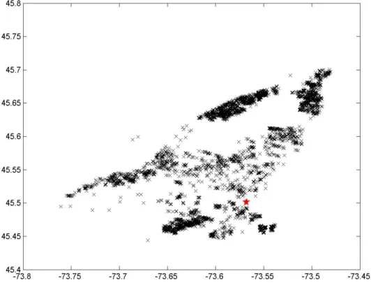
(GIS). Geocoding consists of using specialized software (the GIS) to assign latitude and longitude coordinates to each observation by means of the street address. Af-ter different corrections to address entries, about 80 to 85% of each data set was successfully geocoded and passed to the following filters. Data was then screened to retain only SFH from the old city of Montreal so as to exclude tax and public service variations. All other types of properties were discarded. Transactions after September 2003 were set aside for out-of-sample (OOS) testing. Figure 1 plots the location of these OOS transactions and gives a relative idea of the sales price.
Figure 1: Spatial distribution of out-of-sample transaction data
Note: Size of markers give an indication of price level.
Finally, the remaining entries in the MLS database were used to form two “data groups”: a first one containing only entries with no missing field (‘filtered data’) and a second one containing all valid transactions (‘full data’). Empty fields in this second data group were filed in by matching records to the assessment database for available fields and remaining empty fields were completed by predicted values. All these manipulations yielded two data groups : ‘filtered data’, 4 613 transactions and
‘full data’, 12 770 transactions.
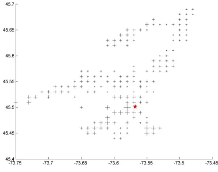
Variables were selected on the basis of previous literature and commonly accepted practice in real estate. All models use the log selling price (in Canadian dollars) as the dependent variable. Explanatory variables for the hedonic portion of all regressions were: log total living area in square feet (LIV), log lot area in square feet (LOT), number of rooms (ROOMS), number of bathrooms (BATHROOMS), a binary variable for the presence of a pool (POOL), number of outdoor parking spaces (PARKINGS), number of garage spaces (GARAGES), distance to city center (DIST), age of the property at time of sale in years (AGE) and following Lesage and Pace (2004), we include its squared (AGE2) and cubic values (AGE3). Dummy variables for the neighborhood and year of transaction were also included. Down town is usually considered to be delimited by four important streets in Montreal (Peel, Sherbrooke, University and Ren´e-L´evesque). City center was therefore defined as the center point of the block circumscribed by these fours streets. Figure 2 plots the transaction data and city center.
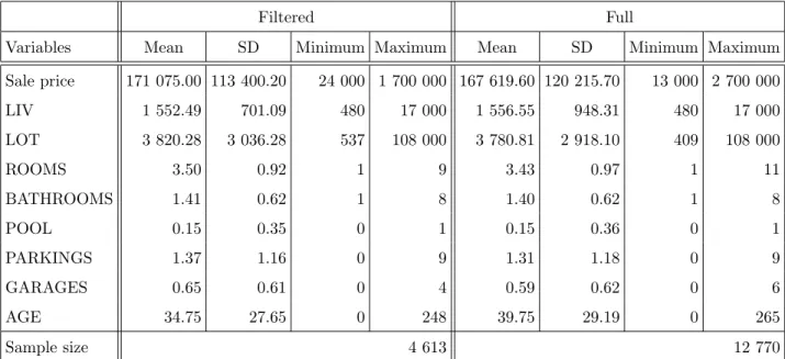
Table 1 report summary statistics for MLS data. Table 2 reports summary statistics for assessment data. All summary statistics are based on the final data sets used for estimation.
By comparing summary statistics, it would seem that observations with missing data do not have much impact on the overall picture. Important variations in the mean are only observed for age. In all other cases, standard errors tend to grow, but means remains very similar. A typical home would be about 40 years old, have 3 bedrooms and about 1 500 square feet.
Figure 2: Spatial distribution of transactions (filtered data) and location of city center
Table 1: Summary statistics of the variables, filtered and full data
Filtered Full
Variables Mean SD Minimum Maximum Mean SD Minimum Maximum
Sale price 171 075.00 113 400.20 24 000 1 700 000 167 619.60 120 215.70 13 000 2 700 000 LIV 1 552.49 701.09 480 17 000 1 556.55 948.31 480 17 000 LOT 3 820.28 3 036.28 537 108 000 3 780.81 2 918.10 409 108 000 ROOMS 3.50 0.92 1 9 3.43 0.97 1 11 BATHROOMS 1.41 0.62 1 8 1.40 0.62 1 8 POOL 0.15 0.35 0 1 0.15 0.36 0 1 PARKINGS 1.37 1.16 0 9 1.31 1.18 0 9 GARAGES 0.65 0.61 0 4 0.59 0.62 0 6 AGE 34.75 27.65 0 248 39.75 29.19 0 265 Sample size 4 613 12 770
Note: LIV and LOT are not log for summary statistics and, in the case of full data, summary statistics are compiled for non-empty fields only .
Table 2: Summary statistics of the variables, assessment data
Assessment
Variables Mean SD Minimum Maximum
FLOORS 1.54 0.53 1 6 SQFT 1 478.44 891.03 298 259 290 LOT 3 666.71 2 930.49 409 197 721 EVALB 115 696.20 89 764.56 5 000 7 686 600 EVALL 62 118.35 52383.82 3 100 3 767 400 AGE 40.67 21.81 1 204 Sample size 44 002
Note: AGE for assessment data is “effective age” as opposed to “actual age” for full data which doesn’t take into consideration renovations made to the property.
3
Methodology
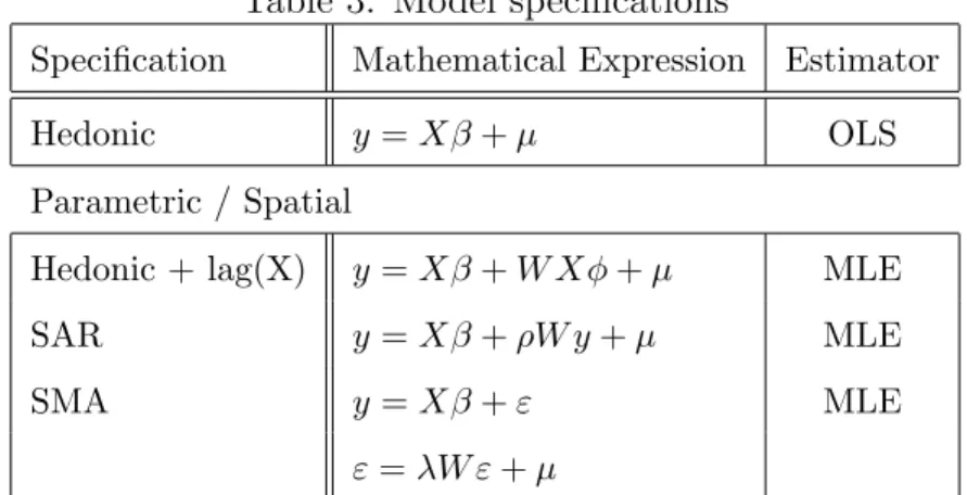
Transactions in the fourth quarter of 2003 were retained for out-of-sample testing to escape the risk of data overfitting. The four specifications mentioned earlier (hedonic model, hedonic model with independent spatial lags, SAR and SMA) were then estimated on remaining data and comparison of results between specification and data sets was conducted. Table 3 presents all four models specifications. Each one is then explained in details in the following sub-sections.
Table 3: Model specifications
Specification Mathematical Expression Estimator
Hedonic y = Xβ + µ OLS
Parametric / Spatial
Hedonic + lag(X) y = Xβ + W Xφ + µ MLE
SAR y = Xβ + ρW y + µ MLE
SMA y = Xβ + ε MLE
ε = λW ε + µ
3.1
Hedonic Model
As described in the introduction, the hedonic approach assumes a relation between market value for sold properties and a particular set of housing characteristics. Here, the hedonic model takes the classic form y = Xβ + µ and is estimated by OLS with Eicker-White robust standard errors. ˆβ can then be used to predict market value of unsold properties with known attributes. y and X may be in log form. For our specification, the dependent variable is the log of the sales price. The model is double-log only for the variables LIV and LOT.
As can be seen in table 3, the linear hedonic specification (y = Xβ. . . ) is present in all other models.
3.2
Basic Spatial Models
Basic spatial specifications add spatial lags to the original hedonic model. These spatial lags can be in the dependent variable y (SAR), the independents variables X or the errors ε (SMA). All three cases are constructed in the same way: by pre-multiplying the desired matrix of variable by a spatial weight matrix W . This (n×n) matrix formalizes the spatial relationship between observations. It assigns weight to “neighboring” observations, so that Wij > 0 for any neighbor j of i. In order
for the observations not to predict themselves, the main diagonal is, by convention, set to zero, i.e. Wii = 0. Finally, to standardize weights, rows of the matrix are
normalized to one.
In the present case, “neighbors” are defined as contiguous observations. Conti-guity is artificially constructed using a Delaunay triangle algorithm, thus insuring that every observation posses a “neighbor”. Kelley Pace’s f delw2 Matlab function is then used to convert the Delaunay algorithm results into a contiguity matrix. Use of a spatial weight matrix based on nearest neighbors did not change the results much.
All spatial models were estimated by MLE. Likelihoods for the three specifica-tions were obtained from Lesage (1999).
3.3
Missing data
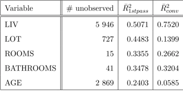
Missing data in the ‘full data’ was completed from assessment data when possible. If corresponding values were not available in the assessment data, missing values were imputed using estimated coefficients from reduced hedonic functions and municipal assessment. These functions took the form: ˆxm = ˆβXo + ˆγEval, where xm is the
missing data, Xo are observed relevant variables and Eval is the municipal
results for these intermediate regressions. Various other specification were tested, spatial and non-spatial, without substantial improvement in data fitting. Most miss-ing data for AGE and LOT was completed with information from the assessment database, but no information was available for ROOMS and BATHROOMS. As-sessment data for LIV was deemed incompatible with that of the MLS database.
Table 4: Intermediate regressions for imputed values
Variable # unobserved R¯21stpass R¯2conv
LIV 5 946 0.5071 0.7520 LOT 727 0.4483 0.1399 ROOMS 15 0.3355 0.2662 BATHROOMS 41 0.3478 0.3204 AGE 2 869 0.2403 0.0585
3.4
Out-of-sample prediction
Out-of-sample predictions were performed for hedonic, hedonic + lag(X)and SAR models. OOS prediction could not be obtained for SMA as errors are unavailable for unobserved data. OOS predicted values were obtained by plugging-in estimated coefficients in each of the models equations.
For assessment data, observed transaction prices for the fourth quarter of 2003 were compared with the assessed value to check for systematic bias. This is equiv-alent to OOS testing as the assessment is supposed to represent the market value as of August 2003. A 25% adjustment was made to all assessments to correct for the systematic reduction described by Cornia and Slade (2003). The choice of the adjustment level was made ex post from the average observed underassessment.
For all OOS predictions, root mean squared prediction error (RMSPE), median absolute prediction error (MAPE) and Theil’s U2 Statistic were calculated to allow
comparison of predictive performance. Theil’s U2 Statistic can be expressed as: U2 = 1 − P (y − ˆy)2 P (y − ¯y)2
Theil’s Statistic is analogue to the R2 and may be used to measure goodness of
fit between actual and predicted house prices. The closer U2 is to one, the closer the forecast error’s variance is to the variance of actual prices.
4
Results
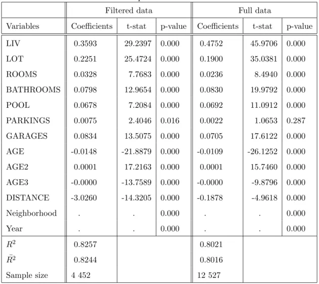
Results for model estimation are presented in tables 5 through 8. Coefficients are all very significant for both data groups. PARKINGS and DISTANCE seems to be the only variable which, for some models, are not significant in the ‘full data’. Other notable variations between the two data groups are the increase in the coefficient of LIV and the reduction of the impact of DISTANCE from city center.
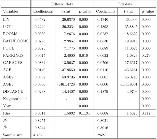
The basic hedonic specification seems to be quite robust since all models exhibit very similar results. Nonetheless, important spatial interactions are detected in the data. Results from LM tests for spatial correlation strongly reject the null hypothesis of no spatial dependence (LM = 589.76, marginal probability < 0.0001). Results tend to point toward spatial autocorrelation of error, what Anselin (2003) refers to as local autocorrelation, rather than global autocorrelation, or autocorrelation in the dependent variable. Indeed, likelihood for the SMA is higher than for the SAR, and λ is strongly significant compared to ρ which barely misses significance at the 10% level.
¯
R2 are quite high for the literature, usual results usually ranging between 0.7
and 0.8. Here, ¯R2 reaches almost 0.85 for the SMA. Basic hedonic model and the
SAR perform only moderately well in comparison. The SAR model shows no real improvement over the basic hedonic model.
Table 5: Hedonic specification estimation results
Filtered data Full data
Variables Coefficients t-stat p-value Coefficients t-stat p-value
LIV 0.3593 29.2397 0.000 0.4752 45.9706 0.000 LOT 0.2251 25.4724 0.000 0.1900 35.0381 0.000 ROOMS 0.0328 7.7683 0.000 0.0236 8.4940 0.000 BATHROOMS 0.0798 12.9654 0.000 0.0830 19.9792 0.000 POOL 0.0678 7.2084 0.000 0.0692 11.0912 0.000 PARKINGS 0.0075 2.4046 0.016 0.0022 1.0653 0.287 GARAGES 0.0834 13.5075 0.000 0.0705 17.6122 0.000 AGE -0.0148 -21.8879 0.000 -0.0109 -26.1252 0.000 AGE2 0.0001 17.2163 0.000 0.0001 15.7460 0.000 AGE3 -0.0000 -13.7589 0.000 -0.0000 -9.8796 0.000 DISTANCE -3.0260 -14.3205 0.000 -0.1878 -4.9618 0.000 Neighborhood . . 0.000 . . 0.000 Year . . 0.000 . . 0.000 R2 0.8257 0.8021 ¯ R2 0.8244 0.8016 Sample size 4 452 12 527
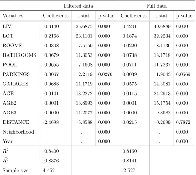
Table 6: Hedonic specification with spatial lag of dependent variables estimation results
Filtered data Full data
Variables Coefficients t-stat p-value Coefficients t-stat p-value
LIV 0.3140 25.6875 0.000 0.4201 40.6889 0.000 LOT 0.2168 23.1101 0.000 0.1874 32.2234 0.000 ROOMS 0.0308 7.5159 0.000 0.0220 8.1136 0.000 BATHROOMS 0.0679 11.3053 0.000 0.0738 18.1718 0.000 POOL 0.0655 7.1608 0.000 0.0711 11.7237 0.000 PARKINGS 0.0067 2.2119 0.0270 0.0039 1.9043 0.0569 GARAGES 0.0688 11.1719 0.000 0.0575 14.3081 0.000 AGE -0.0141 -18.2272 0.000 -0.0115 -24.2913 0.000 AGE2 0.0001 13.8993 0.000 0.0001 15.1754 0.000 AGE3 -0.0000 -11.2077 0.000 -0.0000 -9.8682 0.000 DISTANCE -2.4698 -5.8588 0.000 -0.0215 -0.2699 0.7872 Neighborhood . . 0.000 . . 0.000 Year . . 0.000 . . 0.000 R2 0.8400 0.8150 ¯ R2 0.8376 0.8141 Sample size 4 452 12 527
Table 7: SAR specification estimation results
Filtered data Full data
Variables Coefficients t-stat p-value Coefficients t-stat p-value
LIV 0.3582 29.6370 0.000 0.4746 46.4903 0.000 LOT 0.2249 26.2234 0.000 0.1898 35.8845 0.000 ROOMS 0.0330 7.8676 0.000 0.0237 8.5622 0.000 BATHROOMS 0.0796 12.9857 0.000 0.0830 19.9915 0.000 POOL 0.0673 7.1775 0.000 0.0689 11.0625 0.000 PARKINGS 0.0075 2.4000 0.016 0.0022 1.0823 0.279 GARAGES 0.0834 13.5637 0.000 0.0706 17.6617 0.000 AGE -0.0149 -37.9550 0.000 -0.0110 -43.6251 0.000 AGE2 0.0002 53.9795 0.000 0.0001 46.0743 0.000 AGE3 -0.0000 -1461.4728 0.000 -0.0000 -1144.9601 0.000 DISTANCE -3.0238 -14.4407 0.000 -0.1879 -4.9703 0.000 Neighborhood . . 0.000 . . 0.000 Year . . 0.000 . . 0.000 Rho 0.0014 1.5832 0.1134 0.0008 1.5673 0.117 R2 0.8257 0.8021 ¯ R2 0.8244 0.8016 Sample size 4 452 12527
Table 8: SMA specification estimation results
Filtered data Full data
Variables Coefficients t-stat p-value Coefficients t-stat p-value
LIV 0.3137 35.8127 0.000 0.3964 55.4584 0.000 LOT 0.2230 28.0204 0.000 0.1939 39.1380 0.000 ROOMS 0.0279 7.2243 0.000 0.0231 9.2905 0.000 BATHROOMS 0.0678 11.9881 0.000 0.0749 19.7696 0.000 POOL 0.0659 7.5877 0.000 0.0708 12.4910 0.000 PARKINGS 0.0068 2.4113 0.016 0.0047 2.5245 0.012 GARAGES 0.0695 11.9157 0.000 0.0610 16.1901 0.000 AGE -0.0144 -39.8445 0.000 -0.0118 -54.3144 0.000 AGE2 0.0002 58.2744 0.000 0.0001 63.6876 0.000 AGE3 -0.0000 -6344.6448 0.000 -0.0000 -6149.7125 0.000 DISTANCE -2.6499 -10.1009 0.000 -0.1530 -2.9526 0.003 Neighboorhood . . 0.000 . . 0.000 Year . . 0.000 . . 0.000 Lambda 0.4750 310.6790 0.000 0.4980 361.1253 0.000 R2 0.8497 0.8320 ¯ R2 0.8486 0.8316 Sample size 4 452 12 527
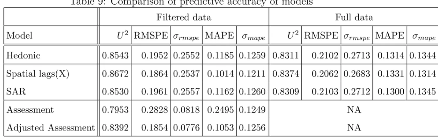
Out-of-sample results tend to confirm the goodness-of-fit of the basic hedonic model. Its Theil’s statistic of over 0.85 for the ‘filtered data’ is surpassed only by the hedonic model with spatial lags of X. Root mean squared prediction error (RMSPE) and median absolute prediction error (MAPE) are also quite good compared to usual results in the literature. RMSPE values of over 0.3 are not uncommon results for real estate predictions.
Table 9: Comparison of predictive accuracy of models
Filtered data Full data
Model U2 RMSPE σrmspe MAPE σmape U2 RMSPE σrmspe MAPE σmape
Hedonic 0.8543 0.1952 0.2552 0.1185 0.1259 0.8311 0.2102 0.2713 0.1314 0.1344
Spatial lags(X) 0.8672 0.1864 0.2537 0.1014 0.1211 0.8374 0.2062 0.2683 0.1331 0.1314
SAR 0.8530 0.1961 0.2557 0.1162 0.1260 0.8309 0.2103 0.2712 0.1300 0.1345
Assessment 0.7953 0.2828 0.0818 0.2495 0.1249 NA
Adjusted Assessment 0.8392 0.1854 0.0776 0.1053 0.1256 NA
The city’s assessment presents the worst goodness-of-fit according to all mea-sures. Once adjusted upward by 25% though, it presents one of the lowest RMSPE and MAPE. Its Theil’s statistic is nonetheless a little lower than that of other es-timated models. Difference in time of evaluation (August 2003) and time of sale could explain part of this disappointing performance.
Using a larger sample with imputed values doesn’t improve OOS predictions either. Statistics show slightly worst results in all instances estimated with “full data”. Further research would be needed to determine if this is due to the data or the imputation method.
5
Conclusion
Results tend to show that the selected hedonic model is subjectively “quite good”. Obtained coefficient are consistent with the literature and goodness-of-fit measures, both in- and out-of-sample are somewhat higher than what is normally found in comparable studies. Spatial models outperform the non-spatial one.
It also seems that the city’s assessment could be improved. Not only are assess-ment largely under market value, even after adjustassess-ment they are outperformed by simple spatial model.
Even though these results are encouraging, much is still to be done. Mass eval-uation techniques tested in this paper would fail to outperform DCC and thus can only be a ‘second best’ when no alternatives exist to mass valuation. Many topics in spatial econometrics are also yet to be addressed. Florax et Vlist (2003) mention many potentially dangerous question that must be tackled in spatial econometrics such as unit roots.
It would also be very interesting to perform the estimations conducted in this research on condos. Models using condos as data are less frequent in the litterature even though condos seem to offer many advantages: a smaller proportion of condo’s transaction data suffers from missing information (43% compared to 65% for SFH in our data), transaction data for condos represents a larger share of total condos than the equivalent for SFH (42% vs. 29%) and, finally, condos exhibit less variation in their characteristics as exhibited by lower standard errors for most variables. Research with this database using condos could thus be a future research agenda.
6
References
Agarwal, D.K., A.E. Gelfand, C.F. Sirmans and T.G. Thibodeau (2001) “Nonsta-tionary Spatial House Price Models”. Working Paper. University of Connecticut.
Anselin, L. (1988) Spatial Econometrics: Methods and Models. Dordrecht, Kluwer Academic Publishers.
Anselin, L. (2002) “Under the hood: Issues in the specification and interpretation of spatial regression models”. Agricultural Economics, 27(3), 247-267.
Basu, S. and T.G. Thibodeau (1998) “Analysis of Spatial Autocorrelation in House Prices”. Journal of Real Estate Finance and Economics, 17(1), 61-85.
Case, B., J. Clapp, R. Dubin and M. Rodriguez (2004) “Modeling Spatial and Temporal House Price Patterns: A Comparison of Four Models”. Journal of Real Estate Finance and Economics, 29(2), 167-191.
Baum A., N. Crosby and P. McAllister, P. Gallimore, A. Gray (2002) “Appraiser behaviour and appraisal smoothing: some qualitative and quantitative evidence”. Paper presented to the Annual Meeting of American Real Estate Society, Naples, Florida.
Bin, O. (2004) “A prediction comparison of housing sales prices by parametric ver-sus semi-parametric regressions”. Journal of Housing Economics, 13(1), 68-84.
Castranova, E. (2004) “The Price of Bodies: A Hedonic Pricing Model of Avatar Attributes in a Synthetic World”. Kyklos, 57(2), 173-196.
Clapp, J.M. (2003) “A Semiparametric Method for Valuing Residential Locations: Application to Automated Valuation”. Journal of Real Estate Finance and Eco-nomics, 27(3), 303-320.
Clayton, J., D. Geltner and S.W. Hamilton (2001) “Smoothing in Commercial Prop-erty Valuations: Evidence from Individual Appraisals”. Real Estate Economics, 29(3), 337-360.
Cornelius, B. (1996) “Valuing Opals: Hedonic Pricing in Practise”. Indian Eco-nomic Journal, 44(4), 122-34.
Cornia, G.C. and B.A. Slade (2003) “Assessed Valuation and Property Taxation of Multifamily Housing: An Empirical Analysis of Vertical and Horizontal Equity and Assessment Methods”. Working paper.
Cressie, N. (1993) Statistics for Spatial Data. revised edition, New York, Wiley ed.
Dubin, R.A. (1988) “Estimation of Regression Coefficient in the Presence of Spa-tially Autocorrelated Error Terms”. Review of Economics and Statistics, 70(3), 466-474.
Dubin, R.A. (1998) “Predicting House Prices Using Multiple Listing Data”. Journal of Real Estate Finance and Economics, 17(1), 35-59.
Florax, R.J.G.M. and A.J. Van der Vlist (2003) “Spatial Econometric Data Anal-ysis: Moving Beyond Traditional Models”. International Regional Science Review, 26(3), 223-243.
Gencay, R. and X. Yang (1996) “A forecast comparison of residential housing prices by parametric versus semiparametric conditional mean estimators”. Economics Let-ters, 52(2), 129-135.
Goolsby, W.C. (1997) “Assessment Error in the Valuation of Owner-Occupied Hous-ing”. Journal of Real Estate Research, 13(1), 33-45.
Hansz, J.A. and J. Diaz III (2001) “Valuation Bias in Commercial Appraisal: a Transaction Price Feedback Experiment” Real Estate Economics, 29(4), 553-565.
Hyman, D. (1998) Public Finance: A Contemporary Approach to Theory and Policy. Fort Worth, Dryden Press.
Jenkins, D.H., O.M. Lewis, N. Almond, S.A. Gronow and J.A. Ware (1999) “To-wards an intelligent residential appraisal model”. Journal of Property Research, 16(1), 67-90.
Kay, J. (1990) “Tax Policy: A Survey”. The Economic Journal, 100(399), 18-75.
King, D.M. and Marisa Mazzotta (2004), “Hedonic Pricing Method”. www.ecosystemvaluation.org
Knight, J.R., C.F. Sirmans, A.E. Gelfand and S.K. Ghosh (1998) “Analyzing Real Estate Data Problems Using the Gibbs Sampler”. Real Estate Economics, 26(3), 469-492.
Lesage, J.P. (1999) The Theory and Practice of Spatial Econometrics. Unpublished Manuscript.
Lesage, J.P. and R.K. Pace (2004) “Models for Spatially Dependent Missing Data”. Journal of Real Estate Finance and Economics, 29(2), 233-254.
Militino, A.F., M.D. Ugarte and L. Garcia-Reinaldos (2004) “Alternative Models for Describing Spatial Dependence among Dwelling Selling Prices”. Journal of Real Estate Finance and Economics, 29(2), 193-209.
Pace, R.K., R. Barry and C.F. Sirmans (1998) “Spatial Statistics and Real Es-tate”. Journal of Real Estate Finance and Economics, 17(1), 5-13.
Palmquist, R. (1980) “Alternative techniques for developping real estate price in-dexes”. Review of Economics and Statistics, 62(3), 442-448.
Palmquist, R. (1991) Hedonic Methods. In Braden, J. and Kolstad, C. Demand for Environmental Quality Amsterdam: Elsevier.
Quan, D. and J. Quigley (1991), “Price Formation and the Appraisal Function in Real Estate Markets”, Journal of Real Estate Finance and Economics 4(2), 127-146.
Rosen, S. (1974) “Hedonic prices and implicit markets: product differentiation in pure competition”. Journal of Political Economy, 82(1), 34-55.