Various Approaches for Solving Problems in Heat Conduction with Phase Change

HAL Id: hal-01120384

https://hal.inria.fr/hal-01120384

HAL is a multi-disciplinary open access

archive for the deposit and dissemination of sci-entific research documents, whether they are pub-lished or not. The documents may come from teaching and research institutions in France or abroad, or from public or private research centers.

L’archive ouverte pluridisciplinaire HAL, est destinée au dépôt et à la diffusion de documents scientifiques de niveau recherche, publiés ou non, émanant des établissements d’enseignement et de recherche français ou étrangers, des laboratoires publics ou privés.

Conduction with Phase Change

Mohamad Muhieddine, Edouard Canot, Ramiro March

To cite this version:

Mohamad Muhieddine, Edouard Canot, Ramiro March. Various Approaches for Solving Problems in Heat Conduction with Phase Change. International Journal on Finite Volumes, Institut de Mathé-matiques de Marseille, AMU, 2009, pp.19. �hal-01120384�

Various Approaches for Solving Problems in Heat

Conduction with Phase Change

Mohamad MUHIEDDINE†?

†_{IRISA, Campus de Beaulieu} ?

Arch´eosciences, UMR 6566 35042 Rennes, France mohamad.muhieddine@irisa.fr

´

Edouard CANOT†

†_{IRISA, Campus de Beaulieu}

35042 Rennes, France edouard.canot@irisa.fr

Ramiro MARCH?

?

Arch´eosciences, UMR 6566 35042 Rennes, France ramiro.march@univ-rennes1.fr

Abstract

This paper treats a one dimensional phase-change problem, ’ice melting’, by a vertex-centered finite volume method. Numerical solutions are obtained by using two approaches where the first one is based on the heat conduction equation with the fixed grid, latent heat source approach (LHA), while the second uses the equivalent thermodynamic parameters

defined by considering the apparent heat capacity method (AHC).

A comparison between the two approaches is presented, furthermore the accuracy and flexibility of the numerical methods are verified by comparing the results with existing analytical solutions. Results indicate that one phase-change problems can be handled easily with excellent accuracies by using the AHC method.

Key words : Phase-change, computational fluid dynamics, fixed grid, latent heat, finite volumes, rolling mesh, self-adaptive mesh, apparent capacity method, moving boundary problem.

Melting processes are classified as moving boundary problems which have been of special interest due to the inherent difficulties associated with the non-linearity of the interface conditions and the unknown locations of the moving boundaries. This paper is concerned with a numerical method for solving a one dimensional phase-change problem leading to further studies on energy-saving and quality im-provements.

Over the years, a number of related computational works have employed various techniques in the analysis of phase change problems. Several important theoretical results on the existence, the uniqueness and the properties of classical solutions are available in the literature [BEJ 03], [MUE 65], [LUI 68], [CAN 67]. Besides, most analytical solutions deal with for 1-D geometries with very particular boundary conditions hence, cannot be generalize to multidimensional problems. Thus, many numerical schemes [KIM 90], [VOL 87], [JAV 06], [SAV 03], [WAN 00], have been proposed to study transient heat conduction problems with phase change in one, two and three dimensions, but two formulations are predominant in the numerical analysis. The first one is referred to as the ’front-tracking method’ in which the position of the moving front is determined at each time step [ASK 87], and must always correspond to a node or edges mesh. The use of this numerical method can usually eliminate the oscillations obtained by using the fixed grid method, and allows for more precise solutions. However, it is poorly suited to multi-dimensional problems due to the algoritm’s difficult implementation and the large computational cost.

The second formulation, based on the use of the heat enthalpy concept [BON 73], [PRA 04], recasts the problem in such a way that the conditions on the moving phase front are absorbed into new equations, and the problem is solved without explicit reference to the position of the internal boundary (interface position). Its position is determined a posteriori, when the solution is complete. The major problem with the latter method is the presence of time fluctuations in the solution. In addition, this formulation often requires the use of algorithms to correct the solution in order not to miss the absorption or the release of latent heat.

Other publications related to heat conduction problems with phase change, using either finite difference or finite element method or both, can be found in references [SAV 03], [GRA 89], [PAW 85]. All of them are of interest, but the most interest-ing numerical method in our case is based on the finite volume formulation which has the important feature that the resulting solution ensures that the conservation of quantities involved such as mass, momentum and energy is exactly satisfied not only over any group of control volumes but over the whole domain of computation, which is not the reality when dealing with finite difference methods. Finite element approach takes advantage in the ability to divide the domain of interest in elemen-tary subdomains, namely elements. It may therefore handle problems with steep gradients and may deal with irregular geometric configurations.

Comparing the advantages and disadvantages of these approaches for the finite volume simulation, this work chooses the fixed grid schemes by using two approa-hes, the latent heat accumulation approach (LHA) [PRA 04] and the apparent heat capacity method (AHC) [BON 73]. The numerical methods based on enthalpy for-mulation of the problem have been studied in [MUH 08], [LAM 04], [BON 73], [PRA

04], [CIV 87]. However, the algorithm proposed for the LHA method is rather simi-lar to that of Prapainop [PRA 04], where the enthalpy formulation has been used to construct an approximation scheme. A comparison between the AHC and LHA ap-proaches will be presented. The finite volume method is implemented over a special rolling mesh in the LHA composed of a fixed regular grid wich is recursively refined near the interface.

1

Mathematical model for simulating problem with phase

change

Only conduction is considered as a heat transfer mode. The physical properties which characterize the solid and liquid phase, such as specific heat and conductivity, are constant for a given phase. In the following, we shortly describe equations for a melting problem, with the further approximation that density is the same for the two phases.

1.1 Equations and boundary conditions

Our melting problem is characterized by solving the partial differential equation obtained by combining Fourier’s law of heat conduction and the law of conservation of energy which states that the rate of energy accumulation within a control volume of size ∆x equals the net heat transfer by conduction

∂ ∂ t

[ρCpT ∆x] = ∆φ (1)

where ∆φ is the heat flux difference at the boundaries of the control volume. The problem deals with a semi-infinite region of ice initially at T0 = −10◦C . At time t > 0, the boundary at x = 0 is suddenly kept at Tw = 20◦C . The governing equations for the temperature T (x, t) are formulated as follows:

   ρCl ∂ T ∂ t = ∂ ∂ x ? kl ∂ T ∂ x ? 0 < x < ξ (t) , t > 0 T_l(0, t) = Tw t > 0 (2)    ρCs ∂ T ∂ t = ∂ ∂ x ? ks ∂ T ∂ x ? ξ (t) < x < +_{∞, t > 0} Ts(∞, t) = T0 t > 0 (3) and for t = 0 T (x, 0) = T0 ∀x ∈ [0, ∞[

where ρ = ρs= ρl is the density, C is the specific heat, ξ(t) is the interface position, and the subscripts s and l indicate the solid and liquid phases, respectively.

At the interface, the heat flux condition is written as [BON 73]:

kl ∂ Tl ∂ x − k s ∂ Ts ∂ x = −ρL dξ dt at x = ξ(t) (4)

where L is the latent heat coefficient and dξ/dt is the velocity of this interface. During the melting process, the liquid/solid front, which absorbs massive latent heat, continuously progresses through the medium. Moreover, the temperature verifies:

Tl= Ts= Tf at x = ξ(t)

where Tf is the melting temperature.

At the initial time, the interface is assumed to be at position zero (i.e., ξ(0) = 0).

2

Analytical solution

Exact solutions of 1D phase change of a semi-infinite slab were analysed by Carslaw and Jaeger [CAR 59] and KU and Chan [KU 90] with the moving front approach. The exact temperature distributions in solid, Ts, and in liquid, Tl, are respectively:

       Ts= Tw+ (Tf − Tw) erf(x∗) erf(x∗ sl) when 0 < x∗ < x∗ sl T l = T0+ (Tf − T0) erfc(?µs/µlx∗) erfc(?µs/µlx∗_sl) when x∗ sl < x ∗ _< ∞ (5)

where x∗ = x/2√µst is the dimensionless position and µ = k/ρC is the thermal diffusivity. The two values are calculated from corresponding mechanical properties for both solid µsand liquid µl values. The values of dimensionless position of solid-liquid interface x∗

sl are obtained via the nonlinear algebriac equation: Tf − T0 Tf − Tw k_l ks ? µs µl exp(−(µs/µl)(x∗_sl) 2 ) erfc(?µs/µlx∗_sl) +exp(−(x ∗ sl) 2 ) erf(x∗ sl) − √ πx∗ slL Cs(Tf − Tw) = 0 (6)

3

Numerical method

The set of equations presented above are cast in the usual finite volume form for a finite domain (actually of length 2 m), under a vertex centered formulation: each cell (or control volume) encloses exactly one data node at xi and its boundaries are always computed as the center of two consecutive nodes, so that we obtain a good accuracy in the gradient estimation. We denote by Ti the whole approximate solution, the location of any variables being indicated by subscripts.

The time domain is divided into an arbitrary number of constant time steps of size ∆t. Variables at time t are indicated by the superscript 0. In contrast, the variables at time level t + ∆t are not superscripted.

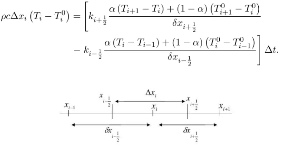
For instance, the temperature at face i + 1

2 is Ti+1 2 = Tifi+1 2 + Ti+1 ? 1 − fi+1 2 ? where f i+1 2 = (2δx i+1 2 − ∆x i)/2δx_i+1 2 , ∆xi = x_i+1 2 − xi− 1 2 , δx i+1 2 = xi+1 − xi, and δx i₋1 2

= xi − xi₋₁ as schown in figure 1). The other variable that has to be approximated at cell faces is the interface conductivity; the harmonic mean is used for composite materials for its superior handling of abrupt property changes by

recognizing that the primary interest is to obtain a good representation of heat flux across interfaces rather than that of the conductivity [PAT 80]:

1 k = 1 − fi+1 2 ki + f i+1 2 ki+1 (7)

In this study, the temporal distributions of temperature is approximated by two-time level schemes [VER 95], such that:

? t+∆t

t

T dt =?αT _{− (1 − α)T}0?∆T (8)

where α is a weighting factor with the value between 0 and 1.

Three main schemes are considered: explicit, Crank-Nicholson and fully implicit. The first-order accurate explicit method uses temperature gradients of the previous time step t to calculate the unknown T at t + ∆t such that α = 0. Hence, the time step size ∆t is limited to ∆t < ρc(∆x)2/2k for 1D. The second-order accurate Crank-Nicholson scheme uses the average of previous and present temperature gradients to compute the present temperature, by taking α = 0.5 in the above, and hence, has less severe step size limitation than the explicit scheme. The fully implicit scheme , however is unconditionally stable with first-order accuracy at α = 1.

Taking Figure 1 as reference, the heat equation may be dicretized as follows:

ρc∆xi ? Ti− T 0 i ? = ? k i+1 2 α (Ti+1− Ti) + (1 − α) ? T0 i+1− T 0 i ? δx i+1 2 − ki₋1 2 α (Ti− Ti−1) + (1 − α) ? T0 i − T 0 i₋₁ ? δx i−12 ? ∆t. (9)

Figure 1: A typical 1D control volume

The convergence and stability of this kind of method could be proven according to the work of [MAG 93].

4

Problem reformulation and Latent heat accumulation

method

In the basic enthalpy scheme, enthalpy is used as the primary variable and the temperature is calculated from a defined enthalpy-temperature relation:

H = ?

ρCsT , T < Tf ρCsTf + ρCl(T − Tf) + ρL, T ≥ Tf

where H is the enthalpy.

Anticipating the discrete description given in the next section, we suppose now that the physical domain (one dimensional in our case) is divided into a finite number of cells (from now on, the subscript i refers to a particular volume).

The latent heat accumulation method has been proposed by [PRA 04] and is resumed hereafter. Prior to the first time interval, the accumulated latent heat Qi of a control volume Ki is initialized to zero. At the beginning of each time step, the phase status of each control volume is checked. If the nodal phase is solid and the nodal temperature Ti rises higher than the melting temperature Tf, then control volume becomes saturated and its node is tagged (the cell is called “mushy”). Since an explicit scheme is used, the current temperature may be calculated directly from the previous values. The nodal temperature is then reassigned to the melting temperature and the latent heat increment (the energy used for phase change in the current time step) is calculated from the fictitious sensible heat such that ∆Qi = ρC (Ti− Tf) Vi, where Vi is the volume of the cell and C is calculated as follows: C = (1_{− θ)C}l+ θCs, where the solid fraction θ is the percentage of ice present in Vi.

The ∆Qi quantity is added to the accumulated Qi for subsequent time steps until the accumulated latent heat equals the total latent heat Qtot

i available in the control volume, which is Qtot i = ? Vi ρLdv (11)

At this stage, the control volume becomes liquid, the tag on the cell is removed and the latent heat increment is no longer calculated.

4.1 Basic model with uniform mesh

As a first step, the discretized formula obtained has been applied under the explicit form where the time step must be chosen according to the Cauchy stability criterion:

∆t < ∆tc = 1 2 ρsCs∆x 2 ks Practically, ∆t is always chosen to be equal to 0.99∆tc.

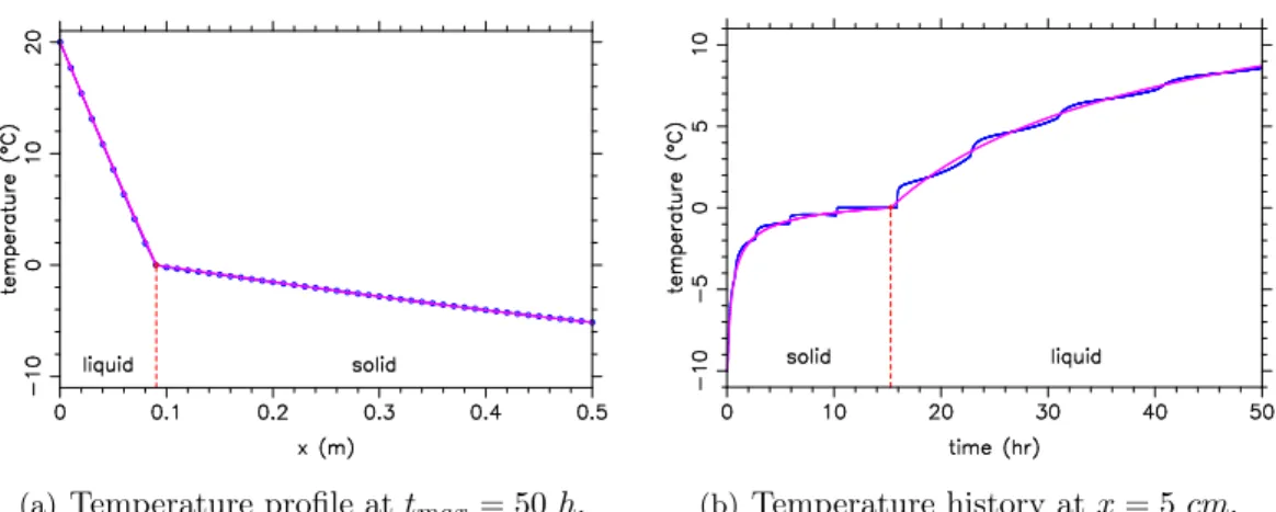
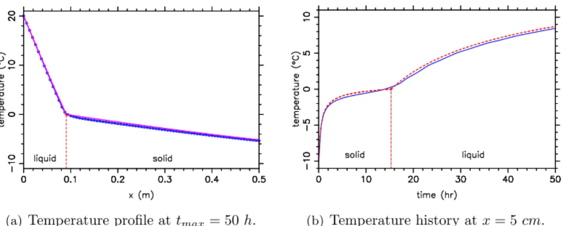
Thermophysical properties used in the calculation are those of the system wa-ter/ice. Spatial temperature profiles (Figure 2a; only a quarter of the whole domain is shown) match the analytical solution [PRA 04] very well, but time evolutions (Fig-ure 2b) present some fluctuations, despite the large number of nodes used. These fluctuations are unavoidable: they are due to the finite width of the cell (In fact, the heat flux is blocked during the melting process inside the mushy cell). To overcome this unwanted behavior, the only way is to refine the grid near the interface, leading to the adaptive mesh technique presented below.

4.2 Improved model with recursive mesh refinement

It becomes obvious that in order to prevent any non-physical solution, it is advan-tageous to vary the mesh size according to the position of the interface. A global

(a)Temperature profile at tmax= 50 h. (b) Temperature history at x = 5 cm.

Figure 2: Uniform mesh, Nbasic= 200, dt = 4.46E + 01 s. Analytical (red) and numerical

(blue) solutions.

refinement would be the simplest technique in order to enhance the accuracy of the approximated solution; however, this technique will not be used here due to the high memory required. In general, two types of adaptive techniques are mostly used; the first one is the local refinement method whereby uniform fine grids are added in the regions where the approximated solution lacks adequate accuracy [ASK 87], and the second is the moving mesh technique where nodes are relocated at necessary time steps [MER 00].

We have chosen a different technique, a classical ’insert/delete nodes’ technique for the primal mesh (like Homard1

, used in FEM but adapted for the finite volume schemes) which has been used with recursive subdivisions, to produce excellent results for the one-dimensional melting problem. The previously described fixed basic uniform mesh is our starting point; then we refine the primal mesh by a number of subdivisions near the phase-change front — at each level of subdivion we add a node at the midle of the two successive nodes (see Figure 3). The melting front is initially located in the first cell and can move anywhere along the discretized domain. When the phase-change front transfers to a new cell, the node added in a previous step is removed and a new node will be added to the new element.

This rolling mesh has the following characteristics:

• the mesh rolls because some nodes are added whereas others are deleted, but only when the mushy cell changes; most of the time the whole mesh remains unchanged;

• only the primal mesh is locally refined; then the dual mesh (i.e., the cell boundary) is updated;

• it is not a moving mesh: during the time evolution all nodes are fixed in position. This fact guarantees a good accuracy due to the small number of needed interpolations (they are needed only when a new node is inserted).

1

This technique was implemented as a double linked list in Fortran 95. Each item of this list contains information about geometry (cell size) and physical variables (temperature, latent heat accumulation and a tag for the phase state). A number of fixed recursive subdivisions is used depending on the precision needs.

Figure 3: Recursive mesh refinement used to track the phase change front (dot points are nodes whereas dashed lines delimit cells; the mushy cell is colored in grey). Blue points are the basic uniform mesh. Circled points are the new nodes which have been inserted (between steps 1 and 2) to satisfy some constraints on the mesh progressiveness. The crossed point disappears between steps 2 and 3.

4.3 Energy conservation during the ’insert/delet nodes’ technique

It is well known that the finite volume scheme conserves some extensive quantities. In our case, it is namely the energy used in equation 1, that can be written as follows

E = ?

ρC T dx (12)

As in our physical model ρ and C are constants (in each phase), the integral of temperature must be conserved over the whole mesh during any ’insert/delete’ nodes event.

Suppose we must insert a new node or delete an existing one: other tempera-ture values at other nodes should be then modified for E to be remain unchanged. However, in our refinement technique (described in the previous subsection), we add/delete a node only for the ’mushy’ cell (corresponding to a slope discontinuity of the temperature) without any modification. This is because a node is always inserted (or deleted) in a linear temperature behavior as we can see in Figures 4a or 5a.

4.4 Results and comments

We have found that the adaptive technique do ameliorates the smoothness (hence the correctness) of the solution. Figures 4 and 5 show numerical results for two different values of the subdivision number. The more we refine the phase-change area, the more we obtain a good accuracy and fewer fluctuations; actually these fluctuations are not eliminated but their amplitude decreases drastically that they seem to vanish (see Figure 7). A good agreement with the analytical solution is shown.

Figure 6a clearly indicates that the local mesh refinement allows the use of a less total number of nodes leading to an economy of memory usage. It also shows errors between the numerical and the analytical solutions, and gives a comparison between

the two models used. The relative error is calculated only from the time evolution curve (at x = 5 cm) via the following Root-Mean-Square formula:

E rrorRM S = ? ? ? ? 1 N N ? j =1 (T (tj) − T (tj)exact) 2 .

N being the total number of time steps.

Globally, taking into account both precision and computational cost, the pro-posed scheme is slightly better than the basic one, as shown in Figure 6b. Actually, the performance limitation of our method is due to the use of an explicit scheme. Therefore this method is poorly suited to multidimensional problem.

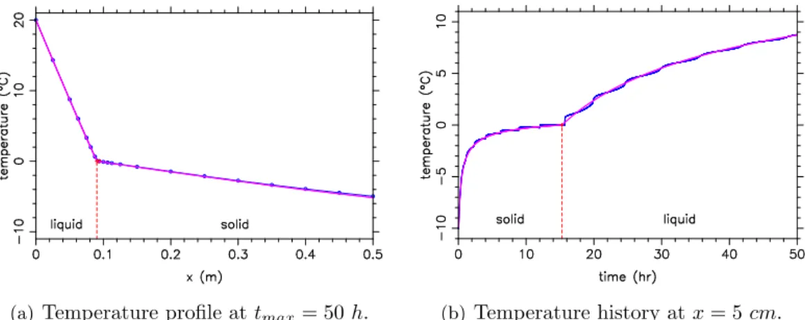
(a)Temperature profile at tmax= 50 h. (b) Temperature history at x = 5 cm.

Figure 4: Rolling mesh, Nbasic = 40, dt = 1.74E + 01 s, Number of subdivisions: 3.

Analytical (red) and numerical (blue) solutions.

(a)Temperature profile at tmax= 50 h. (b) Temperature history at x = 5 cm.

Figure 5: Rolling mesh, Nbasic = 40, dt = 2.72E − 01 s, Number of subdivisions: 6.

Analytical (red) and numerical (blue) solutions.

Due to the limitation of the explicit scheme, several implicit ones have been tried (Crank-Nicholson and a fully implicit scheme) to achieve the expected efficiency and

(a) RMS Errors versus the total number of cells.

(b) RMS Errors versus the computational time.

Figure 6: explicit scheme.

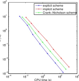
computational cost. As previously described, the explicit scheme has a restriction on time step size. Moreover, large time intervals cause the solution to diverge. Crank-Nicholson and fully implicit schemes may employ somewhat larger time steps but because of the structural model accuracy still depends on time step sizes. In addition, implicit schemes require more CPU time than the explicit scheme due to the iterative procedures of the solver. Figure 8 shows the limitation of the used approach with the implicit schemes, Thus a need of a diferent approach.

10−4 ₁₀−3 ₁₀−2 ₁₀−1 10−1 100 ∆ x_min E rr or m ax ( T (t ))

Figure 7: Oscillations amplitude on temper-ature history. 10−4 10−2 100 102 104 10−3 10−2 10−1 100 101 102 CPU time (s) ε (% ) explicit scheme implicit scheme Crank−Nicholson scheme

Figure 8: RMS Errors on the temperature history versus the CPU time.

5

Apparent heat capacity method

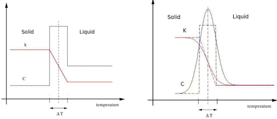
To avoid the tracking of the interface, the apparent heat capacity method will be used. In this method, the latent heat is calculated by integrating the heat capacity over the temperature [BON 73], and the computational domain is considered as one region. As the relationship between heat capacity and temperature in isothermal problems involves sudden changes, the zero-width phase change interval must be ap-proximated by a narrow range of phase change temperatures. Thus, the size of time steps must be small enough so that this temperature range is not overloocked in the calculation. The equivalent thermodynamic parameters are defined considering the apparent capacity method of [BON 73]. According to this reference, if these prop-erties do not depend on temperature, the equivalent parameters may be obtained taking into consideration that the phase change takes place in a small temperature interval (see Figure 9 ).

Figure 9: Physical properties given by Bonacina.

Figure 10: Smoothed physical properties used in this paper.

Then, if this interval is ∆T :

C =    Cs, T < Tf − ∆T Cl+Cs 2 + L 2∆T, T f− ∆T ≤ T ≤ Tf + ∆T Cl, T > Tf + ∆T (13)

Where L is the heat of phase change per unit volume [J/K g], Tf is the phase change temperature, and ∆T is the temperature semi-interval across Tf. Similarly a global new thermal conductivity has to be introduced:

k =    ks, T < Tf − ∆T ks+ kl−ks 2∆T [T − (Tf− ∆T )] , T f − ∆T ≤ T ≤ Tf + ∆T k_l, T > T_f + ∆T (14)

Numerical solutions are obtained by using an approach based on a fixed grid and a vertex-centered finite volume discretization. The accuracy and flexibility of

the present numerical method are verified by comparing the results with existing analytical solutions. The principal advantages of this approach are that (i) temper-ature T is the primary dependent variable which derives directly from the solution, and (ii) the use of this method usually eliminates the fluctuations found by using the LHA approach (see figure 2b). However, the AHC formulation leads to approx-imated solutions and suffers from a singularity problem for the physical properties C (specific heat capacity) and k (conductivity) (see Figure 9). While the explicit form of discretization used in the previous approach is computationally convenient, it has a possible limitation due to the presence of time fluctuations in the solution. Results show the limitation of the LHA method due to the limiting small time step. The implicit calculation is often worthwhile because the implicit Euler method has no stability limit. However, there is a price to pay for the improved stability of the implicit method, which is solving a system of nonlinear ordinary differential equations. We are going to solve PDEs by using the method of lines, where space and time discretizations are considered separatly, leading to semi-discrete systems of ODEs. Fortunately, there is a considerable amount of high quality ODE software available, much of it recently developed. These softwares are used for the integration in t to achieve stability (or a more sophisticated explicit integrator in t is used that automatically adjusts ∆t to achieve a prescribed accuracy).

The numerical solution can be obtained as the limit of a uniformly convergent sequence of classical solutions to approximating problems, deduced by smoothing the coefficients (13, 14), following few general rules [CIV 87]: The apparent heat capacity formulation allows for a continuous treatment of a system involving phase transfer. If the phase transition takes place instantaneously at a fixed temperature, then a mathematical function such as

φ = U (T _{− T}f) (15)

is representative of the volumetric fraction of the initial phase (ice phase). U is a step function whose value is zero when T < Tf and one otherwise. Its derivative, i.e., the variation of the initial phase fraction with temperature, is

dφ

dT = δ(T − T

f) (16)

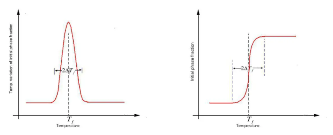
in which δ(T −Tf) is the Dirac delta function whose value is infinity at the transition temperature, Tf, but zero at all other temperatures.To alleviate this singularity the Dirac delta function can be approximated by the normal distribution function sketched in Figure 11 dφ dT = (?π−1/2_)exp[−?2_{(T − T}f) 2 ] (17)

in which ? is chosen to be ? = 1/√2∆T and where ∆T is one-half of the assumed phase change interval. Consequently, the integral of equation 17 yields the error functions approximations for the initial phase fraction as sketched in Figure 12. With conventional finite volume method, the initial phase fraction derived from equation 17 by integration should be used to avoid the numerical instabilities arising from the

Figure 11: Approximation of the initial phase fraction over a small temperature in-terval according to the linear functions.

Figure 12: Approximation of the initial phase fraction over a small temperature in-terval according to the error functions.

jump in the values of the volumetric fraction of initial phase from zero to one. In our approach we assume for simplicity that the phases are isotropic and homogeneous, and the densities of the phases are equal. Accordingly, the smoothed coefficients (see Figure 10) of equations 13 and 14 could be written as:

c = cs+ (cl− cs)φ + L dφ dT (18) and k = ks+ (kl− ks)φ (19)

5.1 Global resolution using the Method of lines

The problem to be solved may be written in vectorial form with adequate initial and boundary conditions:

∂ T ∂ t

= f (t, x, T ) (20)

The user is typically required to write a simple routine which evaluates the func-tion f when the arguments t, x, T , ∂ T /∂ x, ... are provided. Other equally simple subprograms would be required to specify appropriate boundary and/or initial con-ditions.

With generalization in mind, a numerical strategy inspired by the treatment of ordinary differential equations (ODE) associated to space discretization using the method of lines is applied [HUN 03]. It allows:

- a global treatment of the system without discrimination between the variables. - a treatment of the physical model in its original form, as it was written, without preliminary manipulations.

- the use of sophisticated methods wich have been developed for initial value differ-ential equations.

- the possibility, for further works, to use the developments involved in ODE systems (parameter estimation, sensitivity analysis...)

The main failures of the method are the large size of the resulting ODE system obtained after discretization (this problem can be reduced by using an adequate numerical conditioning of the system) and the rigidity of the fixed grid discretization scheme which is not really a problem in our case and could be solved by using an adaptive mesh.

The numerical method of lines consists in discretizing the spatial variable into N discretization points. Each state variable T is transformed into N variables cor-responding to its value at each discretization point. The spatial derivatives are approximated by using a finite volume formula on 3 points where the best results for accuracy and computation time efficiency were obtained. We are solving PDEs, where space and time discretizations are considered separately this lead to a semi-discrete system of ODEs, which can be written as:

T

?

= A(T )T (21)

The Jacobian matrix A(T ) is computed explicitly (its tridiagonal structure is due to the 1-D laplacian discretization). The ODE solver has been modified in such a way that the Jacobian matrix A(T ) could be coded by hand in sparse format. The numerical calculation is performed with ddebdf routine of the SLATEC Fortran library. This is designed to simulate systems of coupled non-linear and time de-pendent partial differential equations. It is used for the time integration to achieve stability and a prescribed accuracy by adjusting automatically the time step in the Backward Differentiation Formula (BDF). The BDF method is well adapted to our problem which becomes more and more stiff as ∆T decreases (see Figure 16).

5.2 Results and comments

The accuracy and flexibility of the present numerical method are verified by com-paring the results with existing analytical solutions [BEJ 03]. Figures 13a and 14a present the temperature profile for different values of ∆T , with spatial discretiza-tion N = 320. Figures 13b and 14b show the related histories of temperature at x = 5 cm. It is evident that the accuracy of the AHC method is sensitive to the magnitude of ∆T that is arbitrarily selected to approximate the Dirac delta function or to distribute the latent heat.

We introduce a quality factor for each solution which combines accuracy and smoothness according to the relation:

Quality factor = E rrorRMS(T ) + 0.025 E rrorRMS(T

?

) (22)

Since the apparent heat capacity method approaches the exact analytical solution as the assumed temperature interval approaches zero, it is shown that the apparent heat capacity method can produce both smooth and accurate solutions.

It appears from these numerical solutions that the results obtained by approx-imating the phase change at a fixed temperature by a gradual change over a small temperature interval should be acceptable if

2∆T |Ti− Tf|

< 0.1 (23)

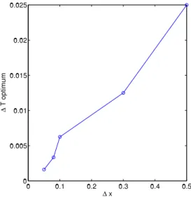
In Figure 15, we can see that there is a minimum for the quality factor corre-sponding to an assumed value of ∆T . This minimum has been drawn as ∆x in Figure 17.

(a)Temperature profile at tmax= 50 h. (b) Temperature history at x = 5 cm.

Figure 13: Nbasic= 300. ∆T = 0.1◦C . Analytical (red) and numerical (blue) solutions.

(a)Temperature profile at tmax= 50 h. (b) Temperature history at x = 5 cm.

Figure 14: Nbasic= 300. ∆T = 0.5◦C . Analytical (red) and numerical (blue) solutions.

6

Comparison between the two methods

Practically in phase change situations, more than one phase change interface may occur or the interfaces may disappear entirely. Furthermore, the phase change

usu-0 0.2 0.4 0.6 0.8 1 0 0.5 1 1.5 2 2.5 ∆ T Q ua lit y F ac to r N = 81 N = 161 N = 321 N = 601 N=1241

Figure 15: Quality factor versus the magnitude of the assumed temperature interval for different number of nodes.

0 0.2 0.4 0.6 0.8 1 0 2 4 6 8 10 12 14 16 18 ∆ T C P U T im e N = 81 N = 161 N = 321 N = 601 N=1241

Figure 16: CPU-Time versus the magni-tude of the assumed temperature interval for different number of nodes.

ally happens in a non-isothermal temperature range. In such cases, tracking the solid-liquid interface may be difficult or even impossible. Calculation-wise, it is ad-vantageous that the problem is reformulated in such a way that the Stefan condition is implicitly bounded up in a new form of the equations and that the equations are applied over the whole fixed domain. This can be done by determining what is known as the enthalpy function H (T ) and by using the AHC approach. The LHA method has the great advantage which is the high precision and the accuracy of the solution, but this method suffers from fluctuations which are covered by a local re-finement of the discretization near the interface. The major problem of this method is that in numerical terms, we are using an explicit parabolic scheme, and this is very penalizing when used with adaptive refinement. For the moment, the problem is solved in 1-D. In 2 and 3 dimensions we can expect ma jor difficulties in terms of implementation and cost.

With the AHC approach, it is also possible to describe the non-isothermal phase change. This proposed model is solved by using the method of lines with which the fluctuations found in the LHA approach can be avoided by choosing an appropriate value of ∆T . Otherwise, it is evident that the error and the order of precision is more pronounced due to approximating the singularity (Dirac delta function) by a gradual change over a small temperature interval. Another observation is that the effect of distributing the latent heat over a temperature interval diminshes as the ratio of temperature interval to the overall temperature variation of the system becomes smaller. It is evident that the AHC method can produce accurate and smooth solutions. Perhaps the biggest criticism to be lodged against this method is that in its normal implementation it requires too much storage for each of the unknown quantities being computed. This would be quite excessive to the person interested in solving a 3-D time dependent problem who is used to needing only several locations per point in the problem.

0 0.1 0.2 0.3 0.4 0.5 0 0.005 0.01 0.015 0.02 0.025 ∆ x ∆ T o pt im um

Figure 17: ∆T optimum versus the ∆x

7

Acknowledgment

This work has been done in the frame of ARPHYMAT2

collaboration., with a fi-nancial support from the ’Minist`ere de l’ ´Education Nationale et de la Recherche, France’.

8

Bibliography

[CAN 67] J.R. CANNON and C.D. HILL, (1967), ”Existence, uniqueness, stability and monotone dependence in a Stefan problem for the heat equation”. J. Math. Mech., Vol.17 pp.1-20

[KIM 90] C. J. KIM and M. KAVIANY, (1990), ”A numerical method for phase-change problems”. Int. J. Heat Mass Transfer., Vol.33 pp.2721-2734

[BON 73] C. BONACINA and G. COMINI, (1973), ”Numerical solution of phase-change problems”. Int. J. Heat Mass Transfer., Vol.16 pp.1825-1832

[PRA 04] R. PRAPAINOP and K. MANEERATANA, (2004), ”Simulation of ice formation by the finite volume method”. Songklanakarin J. Sci. Technol., Vol.26 pp.55-70

[ASK 87] H. G. ASKAR, (1987), ”Simulation of ice formation by the unstructured finite volume method”. Int. J. of Num. methods in engineering., Vol.24 pp.859-869.

[GRA 89] G. M. GRANDI and J. C. FERRERI, (1989), ”On the solution of heat conduction problems involving heat sources via boundary-fitted grids”. Comm. in

2

ARPHYMAT (ARchaeology, PHYsics and MAThematics) is an interdisplinary pro ject involving three laboratories (the two laboratories mentioned in the first page and the GMCM, UMR CNRS 6626).

Appl. Num. Methods., Vol.5 pp.1-6.

[VOL 87] V. R. VOLLER, M. CROSS and N. C. MARKAIOS, (1987), ”An enthalpy method for Convection/Diffusion phase change”. Int. J. Numerical Methods in en-geneering., Vol.24 pp.271-284.

[JAV 06] E. JAVIERRE, C. VUIK, F. J. VERMOLEN and S. Van der ZWAAG, (2006), ”A comparison of numerical models for one-dimensional Stefan problems”. Journal of Computational and Applied Mathematics., Vol.192 pp.445-459.

[SAV 03] S. SAVOVIC and J. CALDWELL, (2003), ”Finite difference solution of one-dimensional Stefan problem with periodic boundary conditions”. Int. J. of Heat and Mass Transfer., Vol.46 pp.2911-2916.

[MUE 65] J. C. MUEHLBAUER and J. E. SUNDERLAND, (1965), ”Heat conduc-tion with freezing or melting”. Appl. Mech. Rev., Vol.18 pp.951-959.

[BEJ 03] A. Bejan and A. D. Kraus, (2003), ”Heat transfer hand book”. Wiley. [LUI 68] A. V. LUIKOV, (1968, New York), ”Analytical heat Diffusion Theory”. Academic Press.

[WAN 00] X. F. WANG, H. S. LIANG, Q. LI and Y. L. DENG, (2000), ”Tracking of a moving interface during a 2D melting or solidification process from measure-ments on the solid part only”. Proceedings of the 3rdWorld Congress on Intelligent Control and Automation., pp.2240-2243.

[MER 00] M. Mriaux and S. Piperno, (2000), ”M´ethodes de volumes finis en mail-lages variables pour des quations hyperboliques en une dimension”. rapport de recherche INRIA, Number 4042.

[PAW 85] I. PAWLOW, (1985), ”Numerical solution of a multidimensional two-phase stefan problem”. JNum. Funct. Anal. and Optimiz., Vol. 8, pp.55-82.

[LAM 04] P. LAMBERG, R. LEHLINIEMI and A.M. HENELL, (2004), ”Numerical and experimental investigation of melting and freezing processes in phase change material storage”. Int. J. of Thermal Sciences., Vol.43 pp.277-287.

[MUH 08] M. MUHIEDDINE and ´E. CANOT, (2008), ”Recursive mesh refinement for vertex-centered FVM applied to a 1-D phase-change problem”. FVCA5.,Aussoie-France, Wiley pp.601-608.

[CIV 87] F. CIVAN and C. SLIEPCEVICH, (1987), ”Limitation in the apparent heat capacity formulation for heat transfer with phase change”. Proc. Okla. Acad. Sci 67, pp.83-88.

[PAT 80] S. PATANKAR, (1980), ”Numerical heat transfer and fluid flow”. Hemi-sphere publishing corporation, New York.

[VER 95] H.K. VERSTEEG and W. MALALASEKERA, (1995), ”An introduction to computational fluid dynamics: the finite volume method”. Longman Scientific and Technical, England.

[MAG 93] E. MAGENES and C. VERDI, (1993), ”Time discretization schemes for the Stefan problem in a concentrated capacity”. Meccanica., Vol. 28, pp.121-128. [HUN 03] W. Hundsdorfer and J. VERWER, (2003, Amsterdam), ”Numerical solu-tionof Time-Dependent advection-diffusion-reaction equations”. Springer.

Clarendon press, London, 282-295.

[KU 90] J.Y. Ku and S.H. Chan, (1990), ”A generalized Laplace transform technique for phase-change problems”. J. Heat transfer, 112: 495-497.